Theory and design of relaxometric probes

RELAXOMETRIC PROBES

Thesis by Carlo Joseph Quiñónez

In Partial Fulfillment of the Requirements for the degree of

Doctor of Philosophy

CALIFORNIA INSTITUTE OF TECHNOLOGY

Pasadena, California

2003

 2003

Carlo Joseph Quiñónez

ACKNOWLEDGEMENTS

First and foremost, I would like to express my deepest gratitude to my family and

friends. Without them, I would not have been able to keep it together long enough to

graduate. Of course I will never forget the support, advice and guidance of my mentor, Prof.

ABSTRACT

In an effort to rationally design an apoptosis-sensitive MRI contrast agent, two novel

gadolinium complexes were designed, synthesized and evaluated as components of a

relaxometric probe. The first, AEDO3A will prove a useful building block for in the area of

the relaxometric probe design. AEDO3A•Gd has a relaxivity of 2.2 mM-1s-1 and 3.4 mM-1s-1

at 60Mhz and 500MHz, respectively. If AEDO3A•Gd is the “on” state and assuming

reasonable relaxivities for the “off” state, tissue contrast modeling of the smallest-detectable

relaxivity change suggests AEDO3A is suitable for incorporation into relaxometric probes.

1-(2-Aspartryl-aminoethyl)-4,7,10-tri(carboxymethyl)-cyclen (Asp-AEDO3A) is

evaluated as the second component of an apoptosis-sensitive relaxometric probe system. The

synthesis and characterization of the ligand and its Gd and Tb complexes is described.

Fluorescence lifetime data of the terbium complex indicate the presence of 0.6 water

molecules in the inner coordination sphere. The gadolinium complex has a relaxivity of

1.4mM-1s-1 and 1.7 mM-1s-1 at 60Mhz and 500MHz, respectively. Toxicity studies

demonstrated Xenopus embryos tolerated Asp-AEDO3A•Gd at magnetically useful

concentrations as predicted by tissue contrast modeling. X-ray crystallography data are

presented for both the ligand and gadolinium complex.

Unfortunately, no enzymatic processing of Asp-AEDO3A•Gd was observed under

any conditions. This phenomenon was attributed to heretofore-unknown coordination

chemistry for gadolinium elucidated from the X-ray crystal structure. This novel

N-carboxamido coordination, while problematic for the application of Asp-AEDO3A•Gd as a

TABLE OF CONTENTS

Acknowledgements...iii

Abstract...iv

Table of Contents ...v

List of Illustrations and/or Tables ...vi

Nomenclature...vii

Chapter I: Introduction...1

Magnetic resonance imaging ...1

Apoptosis: Programmed cell death ...4

Chapter II: Relaxometric probes Relaxivity ...7

Relaxometric probes ...12

Practical aspects...19

Designing an apoptosis-sensitive relaxometric probe...20

Chapter III: Estimation and reduction of errors in relaxivity estimates Introduction ...24

Methods...26

Results ...28

Discussion...31

Chapter IV: AEDO3A – A useful building block for a relaxometric probe Synthesis...33

Characterization ...37

Discussion...40

Chapter V: Asp-DO3A – Attempt at an apoptosis-sensitive relaxometric probe Synthesis...41

Characterization ...45

Discussion...49

Chapter VI: Conclusion Conclusion...50

LIST OF ILLUSTRATIONS AND/OR TABLES

Figures

Number Page

1. Nuclear spins in MRI...2

2. Example of an MRI image ...3

3. Chemical structures of DOTA and DTPA ...4

4. Different coordination spheres of a contrast agent...10

5. Outer-sphere relaxivity ...12

6. q-based relaxometric probe: Metal ion sensitive ...13

7. q-based relaxometric probes: β-galactosidase sensitive ...15

8. τR-based relaxometric probes ...17

9. Scheme for proposed apoptosis-sensitive relaxometric probe...22

10. Distribution of stochastic error used in Monte Carlo simulations ...27

11. Monte Carlo simulation of the uncertainty in relaxivity estimates...28

12. Comparison of ordinary-linear and direct fit algorithms...31

13. Fluorescent lifetime data for AEDO3A•Tb...38

14. Displacement ellipsoid plots for AEDO3A and AEDO3A•Gd...40

15. Fluorescent lifetime data for Asp-AEDO3A•Tb ...45

16. Xenopus embryo injections ...47

17. Displacement ellipsoid plots for Asp-AEDO3A•Gd...48

Tables Number Page 1. Relative magnitude of errors in relaxivity estimates ...30

2. Relaxivities of AEDO3A•Gd ...39

Schemes

Number Page

1. Synthesis of AEDO3A...34

2. Synthesis of Asp-AEDO3A...42

Equations Number Page 1. Longitudinal relaxation time components of water ...7

2. Relaxivity components for a contrast agent ...8

3. Inner-sphere relaxivity ...8

4. Solvent relaxation by SBM theory...8

5. Scalar relaxation by SBM theory...8

6. Dipole-dipole relaxation by SBM theory ...9

7. Local correlation time by SBM theory ...9

8. Electronic correlation time by SBM theory ...9

9. Outer-sphere relaxivity ...11

10. Outer-sphere relaxivity (continued)...11

11. Spectral density function for outer-sphere relaxivity ...11

12. Spectral density function for outer-sphere relaxivity (continued)...11

13. Summed contributions to longitudinal relaxivity of a contrast agent ...13

14. Weighted sum-of-squared deviations ...26

15. Model for direct fit of longitudinal relaxation time data...26

16. Nonparametric method for estimating longitudinal relaxivity ...27

17. Model for the estimation of q...37

NOMENCLATURE

Apoptosis. An active and programmed process of cell elimination vital to homeostasis.

B0. The constant (main) magnetic field of an MRI system. It is usually expressed in

units of Telsa (10,000 Gauss or about 20,000 times the magnetic field of the Earth).

CA. See Contrast Agent.

Contrast Agent. A substance that enhances (shortens) the relaxation time of water molecules, making them appear ‘brighter’ in T1 or T2 weighted MR images. Abbreviated “CA”.

Inner Coordination Sphere. Used to describe any water molecules that are directly coordinated to the metal ion inside a contrast agent.

Larmor Frequency. The Larmor frequency is the frequency of precession of the nuclear magnetic moment (spins) and is proportional to the magnetic field strength as shown in the Larmor equation, ω_I =γ_IB₀, where ωI is the Larmor frequency in Hertz, γI is the gyromagnetic ratio of the nucleus and B0 is the magnetic field strength in Telsa.

MRI. Magnetic Resonance Imaging, a non-invasive technique using strong magnetic fields and radiofrequency pulse to create images of internal anatomy.

NMR. Nuclear Magnetic Resonance, an analytical technique commonly employed in

chemistry.

Outer Coordination Sphere. Used to describe any water molecules that are not in the

inner- or second-coordination spheres.

Pm . The fraction of the solvent bound to the solvent. This is calculated by dividing the

concentration of the contrast agent by the concentration of water (i.e., 55 M), [MCA] 55M .

q. The symbol used to indicate the number of water molecules inside the

inner-coordination sphere, i.e., directly coordinated to the metal ion in a CA.

Relaxation Time. The time it takes nuclear spins to return to their equilibrium state

after excitation by an RF pulse. Intensity in MR image is proportional to relaxation time.

Relaxivity. The ability of a contrast agent to shorten the relaxation time of nearby

water protons. The higher the relaxivity, the shorter the relaxation time.

Relaxometric Probe. A contrast agent that modulates, reversibly or irreversibly, its

relaxivity in response to a physiological stimulus.

Second Coordination Sphere. Used to describe any water molecules that are

coordinated to only the contrast agent ligand, not to the metal ion inside a contrast agent. For

example, a water molecule that is hydrogen bound to a polar group on the ligand.

Smart Contrast Agent. A contrast agent that can serve as a reporter of a physiological

τm. The average length of time a water molecule spends in the inner coordination

sphere.

τR. The rotational correlation time of a contrast agent. This is related to how fast the

contrast is physically tumbling in solution.

T1. The longitudinal or spin-lattice relaxation time. The longitudinal relaxation time is

the time the longitudinal component of the net magnetization vector requires to return to the ground state after excitation by a radiofequency pulse. This is representative of the energy loss associated with high energy spins returning to their low energy state. The longitudinal axis is equivalent to the axis of the external magnetic field (B0).

T2. The transverse or spin-spin relaxation time. The transverse relaxation time is the

time the magnitude of the transverse component of the net magnetization vector requires to return to zero after excitation by a radiofequency pulse. This is representative of the loss of proton spin phase coherence associated with the protons interacting with other protons. The transverse plane is perpendicular to the axis of the external magnetic field (B₀).

C h a p t e r 1

INTRODUCTION

Magnetic Resonance Imaging (MRI) is a non-invasive technique using radio frequency (RF) pulses and strong magnetic fields to create images of internal organs and structures. Computer reconstruction of the data allows high-resolution arbitrary image planes to be generated from a single image imaging procedure. MRI has found applications in almost all areas of medicine, it is used to aid in the diagnosis of cancer, joint and musculoskeletal disorders, and neurodegenerative and cardiovascular diseases.

Apoptosis is an active and programmed process of cell elimination vital to homeostasis. It also has roles in development where the loss of cells serves many functions in deletion of cells and structures [1]. The abnormal activation or repression of apoptosis is also implicated in a wide variety of pathologies [2].

Magnetic Resonance Imaging

sample along the longitudinal axis because of a small excess of spins in the low energy states vs. the high energy state, this net magnetization is best described as a vector. An RF pulse at the Larmor frequency may be used to add energy to the spins, moving spins from the low-energy state to a higher-low-energy state (Figure 1c). Consequently, the longitudinal component of

the net magnetization vector diminishes and eventually becomes negative (against B0) as more RF energy is added to the spins. The relaxation time is the time it takes nuclear spins to return to their equilibrium state. The relaxation time has two components, longitudinal and transverse relaxation times, known as T₁ and T₂ respectively.

The intensity of a magnetic resonance (MR) image depends primarily on three factors – the density of water protons, T₁ and T₂. The visual contrast is determined by the variation in these parameters among tissues. MR images are usually weighed to highlight differences in either T₁ or T₂, otherwise images would be fairly featureless because the density of water does not vary significantly. A small magnetic gradient is added to B0, varying the strength of B0

across sample. Protons within the stronger portion of the magnetic gradient will exhibit a higher Larmor frequency than protons located within the weaker segments. In this manner, spatial information is represented by the Larmor frequency of the protons. The signals from the water protons are detected by a sensitive receiver, and are analyzed by a computerized system to create a visual representation for display on a computer screen. An example of an MR image is presented (Figure 2).

Although satisfactory images are generated using T1 or T2 weighting, it is sometimes

desirable to add additional contrast to an MR image in order to highlight regions of interest. This is accomplished by the use of small molecules called contrast agents (CA). CAs dramatically shorten the T₁ and T₂ of water and their presence is easily detected in MRI images

at levels as low as 0.1 mM. At the core of all CAs is a metal ion such as gadolinium, manganese or iron. Among the ions, gadolinium has the greatest effect on T1 and hence is more

commonly used than the other ions. The unpaired electrons of gadolinium shorten the relaxation time of nearby water protons, making voxels appear ‘brighter’ in T1-weighted

images. Through-space dipole-dipole interactions between nearby water protons and the unpaired electrons cause this enhancement. Unfortunately, gadolinium ions also interfere with calcium-dependant processes and are toxic. Consequently gadolinium is used in the form of a chelate such as DOTA•Gd or DTPA•Gd (Figure 3). Both DOTA and DTPA make gadolinium complexes that are exceedingly stable, ameliorating the toxicity while still allowing the gadolinium ion to affect the T1 of water protons.

Apoptosis: Programmed Cell Death

It is well known cells in the body are constantly being replaced and replenished. In fact, every year a mass of cells equal to the body weight is eliminated in order to make room for these new cells [4]. The cells that are eliminated undergo a process of programmed cell death called apoptosis. This process was first identified and coined in 1972 [5]. Apoptosis Figure 3. Examples of two contrast agents. DOTA and DTPA are polyamino-carboxylate ligands capable of binding gadolinium ions.

literally means “falling leaves” in Greek, relating apoptosis in an organism to the annual shedding of leaves by deciduous tree in the autumn.

Apoptosis is different from necrotic cell death [6]. Although the difference between the two may not always be clear, apoptosis is generally characterized by distinct morphological characteristic such as cytoplasmic shrinkage, chromatin condensation, membrane blebbing and fragmentation into vesicles. There are also extensive biochemical changes that accompany the visible indicators of apoptosis. The composition of the cell membrane changes so that cells undergoing apoptosis are recognized by macrophages that will eventually consume the apoptotic cell. Chromosomal DNA is fragmented and a specific family of intracellular proteases becomes activate. These proteases are collectively known as caspases and disable cellular repair enzymes while activating other downstream proteases to quickly dissemble and package the apoptotic cell for efficient recycling.

Apoptosis can be triggered by many stimuli such as lack of growth factors, hormonal influences or mild toxic insults; active T-cells can also induce apoptosis in other cells. Apoptosis is important to homeostasis and its inappropriate activation or suppression can lead to many different pathologies. Abnormal apoptosis activity has been implicated in immune system disorders [7, 8], carcinogenesis and treatment [9-11], viral infections [12], diabetes [13], stroke [14-16], traumatic brain injury [17, 18], aging [19, 20] and even neurodegenerative diseases [21].

are a family of proteases which were first identified in C. elegans as necessary for programmed

C h a p t e r 2

RELAXOMETRIC PROBES

Relaxometric probes serve as reporters of physiological function by altering their relaxivity in response to a variety of stimuli, such as pH [24, 25], O₂ saturation [26, 27], presence of specific proteins [28, 29], temperature [30, 31], metal ion concentration [32, 33] or enzyme activity [34-37]. These relaxometric probes modulate their relaxivity through a myriad of mechanisms. In order to best appreciate the different mechanisms involved in relaxometric probes, the theoretical basis of relaxivity will need to be explored in some detail.

Relaxivity

In a T1-weighted image, the signal intensity of the voxel will be inversely proportional to the T1 of the water protons contained within that voxel. The observed relaxation time is the sum of the intrinsic relaxation time of the solvent and the contribution from the CA (Equation 1). The superscripts “OBS,” “SOL,” and “CA” are used to respectively indicate the observed, solvent and contrast agent terms.

1 T1OBS

= 1

T1SOL

+ 1

T1CA

[1]

T1CA is modeled as the sum of three independent components (Equation 2). The

superscripts “IS”, “SS” and “OS” are used to respectively indicate the inner-, second- and

outer-sphere contributions to T₁CA. The relaxation time of water molecules in the

T1IS. The relaxation time of nearby water molecules is also affected and their contribution to

T1CAis expressed in two separate terms, T1SS and T1OS.

1 T₁CA =

1 T₁IS +

1 T₁SS +

1

T₁OS [2]

Inner-Sphere Relaxivity

The inner-sphere contribution to T₁CA is given in Equation 3, where q is the number

of water molecules in the inner-coordination sphere, P_m is the fraction of water molecules inside the inner-coordination sphere, τ_m is the average length of time a single water molecule resides within the inner-sphere coordination sphere and T_1m is the relaxation enhancement experienced by the inner-sphere water molecules.

1 T₁IS =

qP_m T_1m+τm

[3]

Solomon-Bloembergen-Morgan theory [38, 39] provides a foundation to understand the basis of T_1m (Equations 4-8). The two components of T_1m term (Equation 4) are dipole-dipole and scalar interactions, noted by the “DD” and “SC” superscripts respectively.

1

T_1m =

1

T₁DD + 1

T₁SC [4]

1

T₁SC =

2

3S(S+1)

A h     _  2

τe2 1+ωs2τe22

(

)

1

T₁DD =

2 15

γH2g2µB2S(S+1) r6

3τc1

1+ωH2τc21

(

)

(

)

      

 [6]

1 τci

= 1

T_ie + 1 τm

+ 1

τR

i=1,2 [7]

1 τei

= 1

T_ie + 1 τm

i=1,2 [8]

The scalar interaction is given in Equation 5. The hyperfine coupling constant A

h     _  is

quite small in most CAs, consequently the contribution of T₁SC to T1m may be safely ignored

and will not be considered further.

Thus T1m is largely determined by the magnitude of the dipole-dipole interactions given

in Equation 6. γH is the proton gyromagnetic ratio, g is the electronic g factor, µB is the Bohr

magneton, S is the number of unpaired electron in the paramagnetic metal ion, r is the distance

between the water protons and the unpaired electrons of paramagnetic metal ion, ωH/ωs are

the Larmor frequencies of protons and electrons respectively, and τ1c, is the local correlation

time of the contrast agent. The electronic contributions (the “7” term inside the square

brackets) may be conveniently ignored because at field strengths used in MRI, ωs2τ_c22 >> 1,

reducing the electronic contributions to an insignificant amount. The nuclear contribution (the

“3” term inside the square brackets) is determined by ω_H2, the proton Larmor frequency, and

τ1c, the local correlation time. The relaxation enhancement efficiency of the CA depends on

frequency of the contrast agent (1/τ_c1). The nuclear contributions to relaxation are maximized

when 1/τ_1c approaches the Larmor frequency of the protons.

The local correlation time (τ_1c) has three components, T1e – the electronic relaxation

time of the unpaired electrons, τ_m – the water residency lifetime, and τ_R – the rotational

correlation lifetime (Equation 7). The high-field strengths used in MRI again simplify matters,

T1e is long enough to reasonably ignore the contributions from the 1/ Tc1 term. τm is the same

term from Equation 3. τR is rotational correlation time and is related to physical tumbling

time of the CA in solution.

Second- and Outer-sphere Relaxivity

Water molecules not directly coordinated to the metal ion also experience relaxation

enhancement in the presence of the CA. These water molecules may be organized into a

second- and outer-coordination sphere (Figure 4). Solomon-Bloembergen-Morgan theory

may also be applied second-sphere water molecules, thus T₁SS may be modeled from

Figure 4. Three coordination spheres, the inner-sphere molecules are directly bound to the

metal, the second sphere consists of water molecules coordinated to other parts of the CA

while the remaining water molecules comprise in the outer sphere.

H2O

N N

N N

O₂C CO₂

N O

O H

H H2O

H2O

OH H

O H H

O H

H O H

H OH

H

H2O

H2O

H2O

H2O

H2O

H2O

Inner-Sphere Molecule

2nd-Sphere Molecules Outer-Sphere

Molecules

Equations 3 and 6. The deviating terms are noted with a prime, e.g., q', r' and τm', to

differentiate them from the unvarying terms, w_H and S. Outer-sphere relaxation enhancement

may be modeled using theories developed by Hwang and Freeman [40, 41]. T₁OS is estimated

using Equations 9-12. Essentially T₁OS is determined by T1e (vide supra), a – the minimum

distance of approach between the metal complex and the outer-sphere water molecules, and D

– the sum of the diffusion constants of outer-sphere water molecules and the CA. The

remaining terms are NA - Avogadro’s Number and M – concentration of CA.

1

T₁OS =C

[

( )

( )

]

C= 32π 405  

  _  γH2g2µB2

(

)

N_aM

1000aD [10]

j(ωi)=Re

1+ 1 4zi 1+z_i+4

9zi2+1₉zi3 

   



  

 i=H,s [11]

z_j = iωj a 2

D + a2

DT_1e i≡ −1, j=H,s [12]

Separating the inner-, second- and outer-sphere components of T₁CA is problematic.

An approach often used to approximate T₁IS of a CA is to simply deduct the T₁CA of a second,

related CA that has q= 0. In the case of the second CA, T₁IS is zero (because q = 0) and the

observed relaxation enhancement is attributed solely to T₁SS and T₁OS. This provides a

expected differ significantly among structurally related CAs. However there are notable

exceptions to this assumption and this approach must be carefully applied (Figure 5).

Presently, there is no satisfactory experimental method to partition the second- and

outer-sphere components of T₁CA

Relaxometric Probes

Relaxometric probes serve as reporters of specific environmental events or conditions

by modulating their degree of the relaxation enhancement. This modulation occurs because

the environmental event or condition alters one or more of the parameters in Equations 2-12.

In order to better understand the potential of the different parameters to affect T₁CA,

Equations 2-12 are condensed and presented into Equation 13. Two reasonable assumptions

Figure 5. Neither DOTP•Gd nor DOTPME•Gd have any water molecules in the

inner-coordination sphere, yet their respective relaxivities are 5.0 mM-1 s-1

and 2.0 mM-1 s-1

. This

disparity is presumably caused by the phosphonate arms of DOTP•Gd that are capable of

forming a more extensive second-coordination sphere.

N N N N P 2-_O 3P PO3

2-P O O O Gd -_O O O -DOTP•Gd DOTPME•Gd H O H H O H H O H H O H H O H N N N N P

EtO₃P PO₃Et

are made in simplifying the equations, [1] 1

T₁SC is omitted because

A h     _  2

≈0 for water

proton-metal interactions in CA’s and [2] 7τc2

1+ωswτc22

(

)

1 T1CA

=kIS

qM 1

S S

(

)

1+ωH

2_τ c1 2      

+τm Inner Sphere Contribution

6 7 4 4 4 4 4 8 4 4 4 4 4

+kSS

′

q M 1

′

r 6S S

(

)

1+ωH

2_{τ ′}

c1 2      

+ ′ τ m Second−Sphere Contribution

6 7 4 4 4 4 4 8 4 4 4 4 4

+kOS

1

S S

(

)

[

( )

( )

]

6 7 4 4 4 4 4 8 4 4 4 4 4

[13]

The overriding criterion for the utility of a relaxometric probe is the change in T₁CA,

therefore parameters that are unfixed are the most relevant. These parameters are q, q', r, r', τc1,

τc1', τm, τm', S and M. The remaining parameters are either physical constants or determined by

B0.

M-based Relaxometric Probes

Recalling that contrast is proportional to 1 T1

, it is desirable to increase M in response

to an environmental trigger because 1 T1CA

∝M. Modulation of M is accomplished in vivo by

designing a CA with a specific affinity for the tissue of interest. In this way, the CA may be

administered systemically but accumulates in specific tissues, increasing the local concentration

for this purpose. This method is perhaps the most straightforward, both conceptually and

practically, although there some difficulties involved with overcoming the low concentration of

antigens and receptors.

q-based Relaxometric Probes

It is desirable to increase q in response to an environmental trigger because 1 T₁CA ∝q.

Modulating q in a relaxometric probe requires altering the coordination environment of the

complex. This has been accomplished via two methods. The first method uses coordinating

groups that bind the paramagnetic metal ion in the CA, serving to displace water molecules

from the inner coordination sphere. These coordinating groups are only loosely bound and

will preferentially bind other metal ions (Figure 6). This mechanism has been used in Ca2+ _and Zn2+ sensitive relaxometric probes [32, 33]. The second method for increasing q is the use of a

group that is not coordinated to the paramagnetic metal ion, but still serves to exclude water

Figure 6. The mechanism for relaxation enhancement in a Ca2+

sensitive contrast agent [32].

In the absence of calcium ions, a loosely coordinated carboxylate fills the coordination

sphere of the gadolinium ion, preventing water molecules from approaching. The addition of

calcium ion removes this blockade.

H2O H2O

H2O

H2O

Ca2+

+

H2O H2O

H2O

H2O

N N

N CO2

-CO2

-CO2

-O O N HO O O O O -N O -O O O O Ca2+ N Gd N N N CO2

-CO2

-CO2

-H2O

molecules by virtue of steric bulk. Two β-galactosidase-sensitive CAs function through this

mechanism [35, 36] (Figure 7A), although data cannot exclude an alternate mechanism

(Figure 7b).

τc1-based Relaxometric Probes (or τR-based Relaxometric Probes)

It is desirable to maximize the nuclear dipole-dipole interations, 3τc1

1+ωHwτc22

(

)

H2O H2O

N N

N N

CO2

-CO2 -CO2

-H2O HO O OH HO OH O OH O OH HO OH OH OH O OH OH HO O OH O OH HO OH OH OH + a) b) O O--O + Gd N N N N

CO2

-CO2 -CO2

-Gd O O--O N N N N

CO2

-CO2 -CO2

-Gd

+

H2O H2O

H2O HO

N N

N N

CO2

-CO2 -CO2

-Gd

Figure 7. Panel A. The action of β-galactosidase removes the galactosyl residue from the contrast agent, thus allowing water molecules to enter the inner coordination sphere. Panel B. Bidentate ligands, such as CO3

or PO4

because 1 T1CA

∝ 3τc1

1+ωHwτc22

(

)



  



   −1

if T_1m >>τ_m. The nuclear dipole-dipole interactions are

maximized when τ_c1= 1 ωH

. τc1 has three components, T1e, τm, and τR (Equation 7), but as

previously pointed out, T1e may be sensibly ignored in most µMRI regimes. Accordingly τ_c1 is

approximately equal to the smallest of τR and τm.

It is generally true in CAs that τ_R <<τ_m and τ_R < 1 ωH

, consequently the short τR is a

limiting factor in 1 T1CA

and lengthening τR is desirable. This has been accomplished dynamically

in relaxometric probes through a myriad of methods (Figure 8). In one example, an enzyme

catalyzed the oligomerization of a relaxometric probe, lengthening τR wherever the enzyme was

active [37]. In another, the relaxometric probe is processed enzymatically into an effective

ligand for a ubiquitous protein, human serum albumin [34]. Different specific receptor-ligand

interactions with DNA-transcription factors [29], carbonic anhydrase [28] or oxyhemoglobin

[27] are utilized in other relaxometric probes. In the final example, the relaxometric probe

undergoes pH-dependant changes to its secondary-structure, altering its τR [24].

Although τm –based relaxometric probes do exist, the fundamental explanation for

their responsiveness in 1

T₁CA is not through modulation of τc1 (vide infra). They will be described

17

Figure 8. Several representations of τR-based relaxometric probes. Panel A.

Enzyme-catalyzed oligomerization increases molecular weight [37]. Panel B.

Thrombin-activatable fibrinolysis inhibitor (TAFI) removes polar amino acids, increasing the

probe’s affinity for human serum albumin [34]. Panel C. A pseudo-inhibitor (a

sulfonamide-derivatized probe) of carbonic anhydrase (CA) forms a non-covalent

adduct with the enzyme [28]. Panel D. A peptide-conjugated probe is recognized and

bound by Gal80, a yeast DNA transcription factor [29]. Panel E. A pH-sensitive

relaxometric probes undergoes extensive remodeling of the secondary structure in response to protonation and deprotonation of the lysine side chains. For example, acidifying the pH would increase the rigidity of the structure as the protonated amines began repelling one another [24].

Note: The “Gd”/hexagon symbol represents a gadolinium chelate and the gray circles represent proteins. a) b) NH O OH OH Peroxidase Gd HN O HO HO Gd NH O OH OH Gd HN O HO HO Gd Gd O HN NH2 OH O 3 TAFI Gd O OH Gd O OH HSA Gd CA c) SO2NH2 Gd SO2NH2 Gd Peptide Gal80 d) Gd Peptide O HN H N HN NH NH HN HN

O NH2O

Gd O O O H2N NH2 Gd Gd e) O N

H H_N

N H HN HN N H HN O

O_O Gd

-HOLDE R

τm-based Relaxometric Probes

In macromolecular CAs, τ_R is sufficiently long so as not to be a limiting factor in 1

T₁CA .

In this case 1

T₁CA is instead limited by τm. This limitation is not a function of the local

correlation time of the complex, τc1, rather it is purely a function of the number of water

molecules cycling through the inner-coordination sphere. The magnitude of 1

T1CA

is limited by

the longest term between T1m and τm in Equation 3. While it is desirable to have τm << T1m so

water exchange rates are never a limiting factor, in practice τ_m is extremely difficult control. In

any case, the limiting effects of slow water exchange in complexes with very long rotational

correlation times has been utilized to make a temperature-sensitive relaxometric probe [31].

S-based Relaxometric Probes

It is desirable to increase S in response to an environmental trigger because 1

T₁CA ∝S if

T1m >>τm . A relaxometric probe which incorporates this mechanisn is a pO2-sensitive

relaxometric probe incorporating a redox-sensitive Mn2+/3+ ion [26]. It should be noted that in

this specific case, the change in S is not the primary mechanism for the relaxation

enhancement, however this serves to illustrate the potential applications of an S-based

Other mechanisms

A relaxometric probe that functions by modulating r has not reported. It is

theoretically possible to modulate r, the design of such a ligand would be difficult. However

even a small change in r, for example 0.2 Å, results in a 30% change in relaxivity because of the

r6_{-dependence of T}

1m.

Deliberate modulation of the second- or outer-sphere contributions in a relaxometric

probe have only been reported in T₂-contrast agents [50, 51]. There are no reports of a T₁

-contrast agent purposely designed to modulate the second and outer spheres.

Finally, there is also an emerging class of CAs have nothing to do with relaxation time.

These CAs utilize chemical-exchange saturation transfer (CEST) pulses to reduce the contrast

wherever they are present. Instead of enhancing relaxation rates, these contrast agents serve as

‘antennas’ for saturating RF pulses that ‘erase’ nearby water protons for a short time from

subsequent MR images, resulting in areas that appear darker than the surrounding tissue in MR

images. For a detailed description of the mechanism, the reader is referred to the published

literature on this subject [52, 53]. Smart CEST agents have been designed that report on

temperature and lactate concentration [54, 55].

Practical Aspects

It would be useful to apply real numbers to these equations to obtain an understanding

of the contributions of τ_m and τ_R in a typical CA. For this purpose we’ll work at a typical

magnetic field employed µMRI (B₀ = 11.7 Tesla), at this field ω_H is 500 Mhz. Starting with

relaxivity of 4.0 mM-1s-1. This CA has τc1= 50 ps, far shorter than the optimal value of 2 ns

(ω−1_H, 500 MHz-1_).

It is valuable to consider how changes in τ_m and τ_R affect the relaxivity. Since τ_R <<

ωH

−1_{, the relaxivity is not limited by slow water exchange. Consequently, shortening τm to}

125ns only increases the relaxivity to 4.1 mM-1s-1, a minimal improvement of .1 mM-1s-1.

Lengthening τR to 100 ps has a more pronounced effect; the relaxivity increases to 7.6 mM-1s-1.

In general for small molecule contrast agents, τR is the primary determinate of relaxivity and τ_m

has very little effect. Only a relatively small number of polyamide derivatives of DOTA and

DTPA have τm’s long enough to adversely affect the relaxivity of small molecule contrast

agents with short τ_R’s.

Linking this CA to a large protein such as albumin will typically lengthen τR to ~2000.

Under these conditions, τc₁ is 1.9 ns – very close to being optimal – and the “theoretical”

relaxivity, T_1m, is 84 mM-1_s-1_{. Unfortunately if} τm _{remains unchanged at 250 ns, the actual}

relaxivity is only 40 mM-1s-1 because it is now limited by the long water exchange time.

Shortening τ_m to 50 ns ameliorates this limitation and increases the relaxivity to 68 mM-1s-1.

Designing an apoptosis-sensitive relaxometric probe

A relaxometric probe will be synthesized and evaluated in an effort to detect apoptosis

in vivo. A q-based relaxometric probe was chosen because of extensive experience with the

design and synthesis of such molecules [32, 35, 36]. In a scheme analogous to prior

relaxometric probes synthesized in this lab, a suitable effector moiety will be attached to

DO3A. The effector moiety would serve to exclude water molecules from inner-coordination

accomplished by the specific action of an enzyme, restoring the relaxivity of the contrast agent

and producing a detectable signal in the MR image.

The first step was choosing the enzymatic target. The criteria for the enzyme are

straightforward, (1) the enzyme must be capable of hydrolyzing a bond and (2) it should

specific to apoptosis. Caspases were immediately identified as the preferred enzymatic target

because their activation is the defining biochemical event associated with apoptosis.

Furthermore, caspases have many aspects that make them an ideal enzyme to target. They are

activated fairly early in the apoptotic cell [56], allowing a longer period for the enzymatic

processing to occur which can be quite prolonged in relaxometric probes. Caspases also have a

relatively short 4 amino-acid consensus sequence and are exo-peptidases rather than

endo-peptidases [57] facilitating the design of the linker between the CA and effector moiety. Finally,

caspases are rather promiscuous enzymes, they can efficiently process a diversity of single

amino-acid substrates including L-Asp, L-Arg, L-Glu and even D-Asp [58]. This also served as

a preliminary indication the enzyme would recognize and process the relaxometric probe being

designed.

Initially the entire consensus sequence for caspase-3 was considered for incorporation

into the relaxometric probe, however when it was discovered that a single aspartate is also an

efficient substrate, the tetra-peptide was dropped in favor of the single amino acid as the

effector moiety. The single aspartate is sufficient bulky to block water molecules from entering

the inner-coordination sphere. Furthermore, the carboxylate side chain and N-terminal amine

blocking water molecules. When the bond between the amino acid and the CA is cleaved,

these inhibitory effects will be removed, restoring the relaxivity.

After the molecular target was chosen, a survey of known CAs was conducted in order

to find one that would serve as suitable building block. Although there are many examples of

CAs linked to peptides or amino acids, this linkage is usually either (1) accomplished by

recruiting a carboxyl group on the ligand to couple to an amine on the peptide [59] or (2)

through a amine group on the ligand located distal to the apical coordination site [60, 61]. A

promising candidate was the ligand 1-(2-aminoethyl)-4,7,10-tri(carboxymethyl)-cyclen

(AEDO3A). Figure 9 illustrates how AEDO3A would be incorporated into a relaxometric

probe.

AEDO3A was chosen because it contains a pendant amine, allowing the attachment of

the effector moiety – the single aspartate – through an amide bond. This amide bond could be

cleaved by a caspase to liberate AEDO3A [62]. Secondly, the length and geometry of the

+ N N N N O O N O O O Gd O N N N N O O HN O O O Gd O O HN O OH OH O HN O OH Aspartic Acid AEDO3A "On" State Asp-AEDO3A "Off" State

Figure 9. _{Proposal for an apoptosis-sensitive relaxometric probe. The Asp-AEDO3A, the “Off”}

pendant amine are likely to place it adjacent to the apical coordination site, maximizing the

likelihood that the effector moiety will be able to efficiently displace water molecules from the

inner-coordination sphere. However, the application of AEDO3A as a CA ligand has not been

reported, therefore the synthesis of the gadolinium and terbium chelates had to be undertaken

to before AEDO3A could confidently be included as a component of the apoptosis-sensitive

C h a p t e r 3

ESTIMATION AND REDUCTION OF ERRORS IN RELAXIVITY

The ordinary linear fit of 1/T₁ vs. concentration has traditionally been used to estimate

the relaxivity of CAs. However, the ordinary linear fit is not well suited to handling 1/T_i data,

errors are neither weighed nor propagated properly. Consequently, errors in the T₁ data do not

‘average’ out and its use should be avoided. Two novel methods of estimating relaxivity are

evaluated as alternatives. The first method is a weighted least-squares fit directly to the T₁ data.

The second method is a distribution-free (or non-parametric) method. A Monte Carlo

simulation used to evaluate the accuracy and precision of each method. Both the direct fit and

distribution-free methods proved more precise than the ordinary linear fit. These novel

methods will prove in reducing uncertainty in relaxivity estimate.

Introduction

The relaxivity change that occurs during the relevant physiological event is a major

criterion for the utility of any relaxometric probe. Tissue contrast modeling suggests that

changes as small as 0.9 mM-1_s-1 _{in the relaxivity of CAs may reasonably be detectable in} T 1

-weighted images [63]. Thus, the precision of the estimates is an important concern when

evaluating the utility of relaxometric probes. Unfortunately relaxivity estimates can be elusive;

for example the relaxivity of a well-known CA, DOTA, has been independently reported to be

anywhere between 3.5 mM-1_s-1 _{[64] and 4.8 mM}-1_s-1 _{[65] – a range of 1.3 mM}-1_s-1 _{which is larger}

than the smallest-detectable relaxivity change in a relaxometric probe system. On the surface,

this uncertainty in the estimation of relaxivity appears to make in vitro evaluation of

for by differences in experimental conditions such as temperature, buffer or field strength.

When measuring relaxivity changes in relaxometric probes, these factors are kept constant and

a comparison between the different relaxivities may more confidently be made.

In order to estimate relaxivity, relaxation times of solutions with differing

concentrations of CA are measured. Relaxivity is defined as the concentration dependence of

1/T₁. The simple linear relationship between 1/T₁ and concentration appears to make the

estimation of r1 a trivial calculation of the least-squares ‘best’ fit line. This is not the case. The

ordinary linear least-squares fit does not properly propagate nor weigh the errors in the data. A

simple non-technical explanation of these points follows. For a more thorough discussion of

these points, the reader is directed to the published literature on these topics [66].

Formal error propagation is necessary when taking the reciprocal distorts errors in T1

data (i.e., it is a nonlinear transformation). Taking the reciprocal of T₁ increases errors in one

direction and decreases them in the other. This becomes readily apparent in an extreme

example such as 1 s ± 0.5 s, the range of possible values is 0.5 s - 1.5 s. Taking the reciprocal

results in 1s-1 with a possible range of 2 s-1 - 0.66 s-1. The error after the reciprocal

transformation is clearly no longer Gaussian, this violates a basic assumption of the linear

least-squares fit. Proper weighing of errors is also important. Most experimental techniques to

estimate T₁ give constant relative errors (i.e., ± 3%) rather than constant absolute error (i.e., ±

5 ms). After the reciprocal transformation, this inadvertently results in points with lower T₁

values (e.g., higher concentrations) being weighed more heavily when estimating the r₁.

This mishandling of errors is a minor, but significant, violation of the assumptions

reasonable estimate of r₁ not the best estimate. Although it is certainly possible to derive the

appropriate corrections to enable the use of a linear fit, it is more expeditious to use a simplex

algorithm to find an r₁ that most closely matches the observed T₁ data. Furthermore, a

non-parametric method to estimate r₁ is proposed and evaluated.

Methods

Linear fit

The linear fit is the traditional method of calculating relaxivities. It is simply the slope

of the best-fit line of 1/T1,i versus [Mi]. This is calculated using the Linest() function in

Microsoft Excel (Redmond, WA). The Y-intercept was not fixed and calculated by the

algorithm.

Direct fit

The direct fit uses a simplex algorithm that iteratively calculates an r₁ that minimizes

the weighted sum-of-squared deviations in T1 (Equation 14).

T1,i−T ˆ 1,i

(

)

ω

i=1

N

∑

The weight (ω) is 1/T ˆ _1,i2 and corrects for the difference in the magnitude of the

variation at different T1’s. The value T ˆ 1,i is calculated (Equation 15) using the empirically

determined T1 of the buffer system as T 01′ .

ˆ T 1,i= _T 1_′

01

−r1,i[Mi]

 

 

 

−1

This model was constructed using Excel and solved using a simplex algorithm

accessed via the Solver plug-in. A sample spreadsheet of this model is included in the

Appendix.

Distribution-free method

The distribution-free method calculates r1,ij (Equation 16) for all possible pairs of T1’s

in the data set and returns the median (not the average) value. There are (N)*(N-1)/2 unique

pairs in a data set consisting of N samples. For example, in a data set consisting of three CA

concentrations {(T1,a,[Ma]), (T1,b,[Mb]), (T1,c,[Mc])} and one blank measurement {(T01,d,[0.0])},

there are six unique pairs of data. (i.e., A-B, A-C, A-D, B-C, B-D, C-D). The relaxivity for each

unique pair is calculated and median value is considered the relaxivity of the CA. A sample

spreadsheet of this model is included in the Appendix.

r1,ij = 1

T1,i

− 1

T1,j

M_i

[ ]

[ ]

Monte Carlo Simulations

The Monte Carlo simulation was performed using Excel. Theoretical T₁ values were

calculated from Equation 3 (r1 = 3.1 mM -1

s-1, T01 = 2.0 s) at several concentrations of CA. An

‘observed’ T₁ was calculated by introducing stochastic errorinto the theoretical T₁. The error

was randomly generated for each individual data point and was normally distributed (Figure

10) with a fixed mean and standard deviation. The relaxivities were then estimated using the

linear fit, direct fit and the distribution-free methods.

The simulations were performed under a variety of error conditions (SD= 2.5%, 5%,

10%) and data set sizes (N=2-7).

Results

The results of simulated relaxivity estimates were analyzed to ascertain their accuracy

and precision (Figure 11). For example, if one uses 6 data points and assumes 5% error in the

underlying T1 data, then the error in the relaxivity estimate will be approximately ± 4.6% using

the direct fit or ± 9.5% using the linear fit. Although the difference in accuracies (data not

Figure 11. Distribution of relaxivity estimates produced by the direct fit (solid line),

distribution-free method (short dashes) and the ordinary linear fit (long dashes) for data sets

consisting of 3, 6 or 12 concentrations (Panels A, B and C, respectively). These curves

shown) between the methods is statistically significant because of the large sample sizes used in

the simulations, the magnitude of the differences, less than 0.5%, is not relevant to most

discussions of CA relaxivity. Hence when judged solely on the basis of accuracy, all methods

performed equally well.

However, the precision of relaxivity estimates differed by a noteworthy amount. As

expected, the direct fit returned the most precise estimates while the linear fit performed the

worst. Indeed, using linear fit is not much better than simply estimating relaxivity solely from

most concentrated sample – regardless of the actual number of concentrations used in the fit.

This is expected from the incorrect weighing of the individual data points and is borne out in

the Monte Carlo simulations.

The direct fit estimates were the most precise of the three methods evaluated. Directly

comparing T₁ and T ˆ ₁, as opposed to 1/T₁ and 1/T ˆ ₁ in the linear fit, avoids the confounding

reciprocal transformation required in the linear least-squares estimation. Furthermore, the

variation at each [M_i] is weighed for more accurate treatment of error. Consequently, the

precision of the direct fit method increases with increasing number of data points used. As one

would expect, this decrease in variation is roughly proportional to the square root of the

number of data points used.

In contrast to the direct fit method that assumes a normal distribution of error and a

constant proportional variance, the distribution free method uses a much simpler assumption

– positive errors are as likely as negative errors. The detriment to this method is that it

produces a weaker conclusion (more uncertainty) because it relies upon weaker assumptions.

will always produce results that are more

precise. However, a non-parametric analysis

such as the distribution free method will

provide better estimates, in general, than a

poorly chosen parametric analysis, as is the

case with estimating relaxivity with the

linear fit.

Goodness of fit is best assessed

visually (Figure 12). The reciprocal plot of

T1 can be misleading because it visually

distorts the magnitude of the error in all the

data points and gives misleading

information to the viewer about the

goodness of fit. Neither is the direct plot

ideal either for the visual inspection of the

goodness of fit. A plot of the weighted

residuals [1−

(

)

visual indicator of goodness of fit. It is vital

to consider that the data in Fig. (2) contains

a reasonable amount of error (5%) and the

Linear Fit appears optimal, yet the error in

the resulting relaxivity estimate is 8.4%. This

N Direct Fit Linear Fit Distribution Free 2.5% Error

2 1.71% 2.55% 2.55% 3 1.64% 2.61% 1.94% 4 1.42% 2.68% 1.84% 5 1.32% 2.48% 1.84%

6 1.10% 2.32% 1.68% 8 3.77% 8.36% 6.04% 10 0.77% 1.91% 1.33% 12 0.72% 1.75% 1.19%

5% Error

2 3.65% 4.94% 4.94% 3 3.42% 5.45% 4.06% 4 2.87% 5.10% 3.52% 5 2.52% 4.90% 3.58%

6 2.29% 4.77% 3.29% 8 1.89% 4.25% 2.98% 10 1.62% 3.92% 2.73% 12 1.40% 3.46% 2.29%

10% Error

2 7.39% 10.45% 10.45% 3 6.52% 10.65% 7.84% 4 5.87% 11.06% 7.58% 5 4.90% 10.35% 7.23%

6 4.39% 9.26% 6.39% 8 3.77% 8.36% 6.04% 10 3.25% 8.22% 5.57% 12 2.72% 7.30% 4.75%

Table 1. The standard deviations of the various simulated relaxivity estimates are

presented. Each line in the table presents

standard deviations (expressed as a

percentage) of relaxivity estimates generated

by the three methods using 2000 sets of T1

data with the stated error and number of

data points (not including the blank). These

values are useful for approximating the error

in individual relaxivity estimates because

95% of the time the ‘true’ relaxivity will be

highlights the uncertainty present in relaxivity estimates regardless of the visual appearance of

the plotted data.

Discussion

The errors associated with estimating relaxivities are numerous and the statistical

model used should reduce these errors. The ubiquity of Excel and other spreadsheets make the

calculation of the direct fit and distribution free methods only slightly more laborious than the

Figure 12. Panels 2a and 2b present reciprocal and direct plots of the following T1 data ([Mi],

T1,i) = [(0 mM, 1.93 s), (0.63 mM. 405 ms), (1.25 mM, 246 ms), (2.5 mM, 122 ms), (5 mM, 59.1

ms), (10 mM, 29.6 ms)] with superimposed Direct and Linear Fits using T01 of 1.93 s. This T1

data was generated from a ‘true’ r1 of 3.1 mM-1

s-1

with a random error (εi) = (0.932, 0.946,

1.000, 1.078, 0.988, 0.969). Panel a. The Linear Fit (dashed line) appears to fit the data quite

well, while the Direct Fit (solid line) seems to miss the 5mM and 10mM points. Panel b. The

direct plot is not better for judging the goodness-of-fit. The difference between the two fits

appears minor. Panel c. The plot of the weighted residuals is the most useful visual indicator of

goodness of fit. The residuals from the direct fit appear centered on the X-axis while residuals

from the linear fit lie mostly above the X-axis. Although visually the differences appear minor,

the calculated relaxivities from the Linear and Direct Fits are 3.36 mM-1

s-1

and 3.12 mM-1

s-1

respectively. For comparisons sake, the Distribution Free method estimated a relaxivity of 3.31

mM-1

s-1

linear fit. The use of the linear fit should be avoided and either the direct fit or distribution free

method substituted in its place. The direct method provides the most precise estimates of

relaxivity, however like all parametric methods it is sensitive to outliers. Because visually

detecting outliers or assessing the goodness of fit is difficult, unless residuals plots are

inspected the distribution free method should be employed. This method handles errors,

including outliers, in a robust manner yet still produces more precise estimates than the linear

fit. The uncertainty reported in relaxivity should reflect the number of concentrations used in

C h a p t e r 4

AEDO3A – A USEFUL BUILDING BLOCK FOR A RELAXOMETRIC PROBE

1-(2-Aminoethyl)-4,7,10-tri(carboxymethyl)-cyclen (AEDO3A) is evaluated as a

component of a relaxometric probe system. The synthesis and characterization of the ligand

and its Gd and Tb complexes is described. The gadolinium complex has relaxivities of

2.2mM-1s-1 and 2.4 mM-1s-1 at 60Mhz and 500MHz respectively. Fluorescence lifetime data of

the terbium complex indicate the presence of 0.9 water molecules in the inner coordination

sphere. X-ray crystallography data are presented for both the ligand and gadolinium complex.

Assuming reasonable relaxivities for the “off” state, tissue contrast modeling of the

smallest-detectable relaxivity change suggests AEDO3A is suitable for incorporation into relaxometric

probe the desired relaxometric probe.

Synthesis

Attempts to synthesize this agent using the literature procedure produced

unsatisfactory yields in this laboratory. Consequently, a new synthetic route (Scheme 1) was

developed that required neither silica-gel chromatography nor HPLC to purify intermediates.

AEDO3A was synthesized in four steps starting from bromoethylamine. The

2-bromoethylamine was acylated with BOC-anhydride to yield the BOC-protected derivative (1)

that was then reacted with a 5-fold excess of cyclen to promote monoalkyation. Compound 2

was exhaustively alkylated with t-butyl bromoacetate to yield the fully protected ligand 3.

Deprotection using TFA yielded the final ligand 4. The final complexes, 5a and 5b, were

final complexes were purified by precipitation followed by column chromatography (Biorad

Chelex) and dialysis to remove any trace heavy metals.

All reagents and solvents were purchased from Aldrich, Fluka, or Strem (cyclen) and

were used without further purification. Ion exchange resins purchased from Bio-Rad.

N-Boc-2-aminoethyl bromide (1). A 1N solution of sodium hydroxide (160 ml) was

added dropwise over 15 minutes to a vigorously stirring biphasic system of bromoethylamine

hydrobromide (17.85 g, 87.1 mmol) in water (100 ml) and di-t-butyl pyrocarbonate (9.5 g, 43.5

mmol) in dichloromethane (100 ml). After 2 hours, the layers were separated and the organic

layer was washed with 1H HCl (25 ml) twice and a saturated sodium chloride (25 ml) once.

The organic layer was then dried over sodium sulfate and concentrated in vacuo to a colorless

oil. The oil was dissolved in hexanes (10ml) and placed at –80° C overnight. 1.9 grams of a

Br NHBoc _NHBoc HN NH N NH NHBoc N N N N t-ButylO O

Ot-Butyl O

O Ot-Butyl

N N N N O -_O O -_O O O -NH2

5a M=Gd3+ 5b M=Tb3+ 1 N N N N O HO O HO O OH NH2 4 M 2 3 Br NH2

a b c

d e

Scheme 1: Synthetic Scheme for AEDO3A. a) BOC-anhydride, NaOH, DCM/H2O, yield 70%; b)

cyclen, MePh, yield 56%; c) t-Butyl bromoacetate, Na2CO3, yield 85%; d) TFA,

white solid that crystallized was filtered and washed with cold hexanes. The combined filtrates

were again placed at –80°C for 1 hour to precipitate a second batch of crystals weighing 4.9

grams. Total yield, 6.8 grams (30.3 mmol or 70% yield). 13C NMR (CDCl3, 300 MHz) δ 155.6,

79.8, 42.3, 32.8, 28.3. 1H NMR (CDCl3, 300 MHz) 5.03 (s, 1H), 3.53 (t, 2H), 3.46 (t, 2H), 1.46

(s, 9H). HR-CI+GC, m/z 224.0286 (M+H) theoretical 224.0286.

(N-Boc-2-aminoethyl)-cyclen (2). A solution of 1 (10.3 g, 45 mmol) and cyclen (30.96

g, 180 mmol) in toluene (400 ml) was stirred at 70°C overnight. The following day, the product

was extracted from the reaction mixture using water (100 ml, 4x). The combined aqueous

layers were washed with toluene (50 ml) followed by dichloromethane (100 ml, 4x). The

dichloromethane layers were combined, dried over sodium sulfate and then concentrated in

vacuo to a colorless oil. The oil was dissolved in dichloromethane (15 ml), diethyl ether was

added until the solution was cloudy and placed at -80°C overnight. The white solid that

precipitated was filtered and washed with cold ether. Total yield, 7.5 grams (24 mmol, 56%

yield). 13C NMR (CDCl3, 300 MHz) δ 155.99, 81.73, 80.43, 50.66, 41.17, 37.17, 31.67, 28.32,

28.04. 1H NMR (CDCl₃, 300 MHz) 5.65 (s, 1H), 3.21 (q, 2H), 2.72-2.48 (m, 21H), 1.44 (s, 9H).

HR-FAB, m/z 316.2728 (M+H) theoretical 316.2712.

(N-Boc-2-aminoethyl)-4,7,10-tri(t-butoxycarbonylmethyl)-cyclen (3). A solution

of 2 (950 mg, 3 mmol), sodium carbonate (3.3 g, 31 mmol) and t–butyl bromoacetate (2.4 ml,

15 mmol) in acetonitrile (100 ml) was stirred at 70°C overnight. The following day, the

reaction was filtered and washed with heptane (250 ml, 3x). The acetonitrile layer was then

concentrated in vacuo to a pale yellow oil. The oil was dissolved in dichloromethane (15 ml),

solid that precipitated was filtered and washed with heptane. Total yield, 1.68 grams (2.5 mmol,

85% yield). 13_{C NMR (CDCl}

3, 300 MHz) δ 173.36, 172.84, 172.58, 156.42, 82.80, 81.42, 81.94,

79.20, 56.51, 55.69, 53.95, 50.34 (m), 37.84, 28.41, 28.01, 27.82. 1_{H NMR (CDCl}

3, 300 MHz)

5.43 (s, 1H), 3.4 - 2.2 (m, 26H), 1.6-1.4 (m, 36H). HR-FAB, m/z 658.4750 (M+H) theoretical

658.4754.

1 -Ami noethyl-4 ,7,10 -tri(carboxymethyl)-cyclen (4 ). A solution of 3 (1.6 grams, 2.5

mmol) in triisopropyl silane (500 µl) and trifluoroacetic acid (50 ml) was stirred overnight at

room temperature. The following day the solution had turned orange and the solvent was

removed in vacuo until less than 1 ml remained. The remained solution was added dropwise to

cold diethyl ether. The pale orange solid that formed immediately was filtered, and then

resuspended in a minimal amount of water (~3 ml). The final product was titurated and

filtered off by the addition of a large excess of acetone (~100 ml). Total yield, 420 mg (1.1

mmol, 45% yield). 13C NMR (D₂O, 500 MHz) δ 175.70, 170.50, 57.31, 52.69, 52.27, 50.60,

50.30, 48.39, 48.17, 36.29. 1H NMR (D₂O, 500 MHz) 3.8-2.6 (m). HR-FAB, m/z 390.2355

(M+H) theoretical 390.2352.

1 -(Ami noethyl)-4 ,7 ,1 0-tri (carboxymethyl)-cyclen, gadoli ni um salt (5 a). A solution

of 4 (289 mg, 743 µmols) and gadolium chloride (235 mg, 891 µmols) was stirred at 80° C

overnight. The pH was periodically checked and adjusted to 6.0~7.0 using a solution of

lithium hydroxide (1M) as needed. After 12 hours, lithium hydroxide was added to bring the

pH to ~12 and reaction was syringed through a nylon .2 µm filter. The filtrate was then

lypohilized to a white powder that was resuspended in a minimal amount of methanol (~1 ml).

The final product was titurated from this solution and filtered off by the addition of a large

Chelex), dialyzed (100 MWCO) and lyophilized to an off-white powder. Total yield, 242 mg

(446 µmols, 50% yield). HR-FAB, m/z 545.1361 (M+H) theoretical 545.1358.

1-(Aminoethyl)-4,7,10-tri(carboxymethyl)-cyclen, terbium salt (5b). This

compound was made in a fashion similar to 5a. Total yield, 325 mg (596 µmols, 80% yield).

HR-FAB, m/z 546.1384 (M+H) theoretical 546.1376.

Characterization

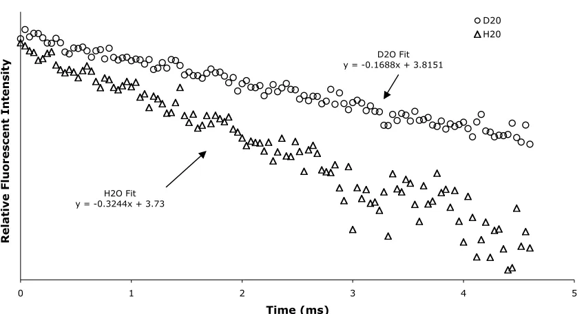
The number of water molecules in the inner-coordination sphere (q) was indirectly

determined by measuring the fluorescent lifetimes of 5b in H₂O and D₂O (Figure 13). The

O-H oscillators present on the coordinated water molecule are efficient quenchers of the excited

state of 5b. However O-D oscillators are largely ineffective at quenching fluorescence,

therefore it is possible to indirectly determine the number of water molecules in both

coordination spheres by measuring the fluorescence lifetimes in D₂O vs. H₂O [67]. Nearby

water molecules in the outer coordination sphere also quench the excited state, albeit to a

lesser extent because of their relative distance from the metal center. This relationship between

the fluorescent lifetimes is modeled in Equation 17 [68, 69].

q=5

(

)

When the published correction factors for the presence of inner-sphere N-H

oscillators were incorporated into Equation 17, q was 0, which is unreasonable considering

the crystallographic evidence to the contrary. The uncorrected lifetime data was used instead,

results are also indicative of the equilibrium distribution of the complex where there is one or

no water molecules bound.

The spin-lattice relaxation times (T₁) of the bulk water were measured in order to

estimate the relaxivity (r1) of 5a. The relationship between T1 and r1 is given in Equation 18,

where T₁OBS is the half-life of the inversion recovery process. r₁ was estimated by the use of a

simplex algorithm.

1

T₁OBS = 1

T₀₁+r1[M] [18]

Because relaxivities varies with field strength (Table 2), measurements were made at

several common field strengths used in both MRI and µMRI applications. The buffer system

with phosphate and carbonate anions most closely resembles in vivo conditions, while the Figure 13: Fluorescent Lifetime Data of AEDO3A-Tb.

3 4 5 6 7 8

0 1 2 3 4 5 6 7 8 9 10

Time (ms)

Relative Fluorescent Intensity

D20 H2O

H2O Fit

y = -0.6559x + 7.8181

D2O Fit

second facilitates comparison with relaxivities of other CAs that were measured in

phosphate-and carbonate-free buffer systems [70, 71]. These numbers are typical of a small-molecule CA

with a single coordinated water molecule [72].

Using a model for MRI contrast enhancement for T1 agents it is possible to evaluate

the utility of 5a as the “on” component of a relaxometric probe [63]. Using the r1 data

obtained for 5a, the relaxivities for the “off” state that will lead to an acceptable signal-to-noise

at an intracellular concentration of 1mM were estimated to be 1.6 mM-1s-1, 1.9 mM-1s-1, 2.2

mM-1s-1 or 1.8 mM-1s-1 at 60MHz, 300MHz, 500MHz and 600MHz, respectively. These

relaxivities represent the smallest-detectable relaxivity change in the Xenopus (African horned

frog) embryo. Given the relaxivities of other “off” contrast agents [35, 36] and some q = 0

complexes [72], it seems reasonable to achieve the desired relaxivity of the “off” component of

the relaxometric probe.

Single crystals of 4 and 5a were obtained by the slow diffusion of acetone into aqueous

solutions of the compounds. X-ray crystallography confirmed the structures (Figure 14).

Compound 5a crystallized with two conformational isomers (labeled A and B) in the

asymmetric unit. The two isomers differed mainly because of an inversion of the ethylene

Field Strength (MHz) Relaxivity (mM-1_s-1₎

Buffer A Buffer B

60 2.2 2.6

300 2.6 4.0

500 2.4 4.0

600 2.4 3.1

Composition of buffer

10 mM MOPS 100 mM NaCl

4 mM Na2CO3 20 mM Na3PO4

10 mM MOPS 100 mM NaCl

linker to the pendant amine. The torsion angle GdA-N4A-C15A-C16A was 53.8° while

GdB-N5B-C15B-C16B was 12.3°. The coordinated atoms are arranged in a monocapped twisted

square antiprism, with N1A, N2A, N3A and N4A composing one plane (rms deviation =

0.0170 Å) 1.638 Å below GdA while N5A, O1A, O2A, O3A and N5A line on the second

plane (rms deviation = 0.0352 Å) 0.762 Å above GdA. The planes are twisted approximately

37° relative to each other.

Discussion

We succeeded in the synthesis and characterization of gadolinium and terbium

complexes of AEDO3A. The relaxation and fluorescent lifetime indicate a potential for the

inclusion of AE-DO3A-Gd into a relaxometric probes. The cystallographic data indicate the

pendant amine is coordinated to the metal center, a favorable position to serve as an anchor

for an effector moiety expected to modulate the inner coordination sphere.

Figure 14. Displacement ellipsoid plots of 4 and 5a with 50% surfaces. Selected bond

lengths from 5a: Gd-N5A = 2.597(2) Å, Gd-N5B = 2.560 Å, Gd-N(1-4)(A-B) = 2.637(2) –