Private Projections & Variants
Xavier Carpent
University of California, Irvine
[email protected]
Sky Faber
University of California, Irvine
[email protected]
Tomas Sander
Hewlett Packard Labs
[email protected]
Gene Tsudik
University of California, Irvine
[email protected]
ABSTRACT
There are many realistic settings where two mutually suspi-cious parties need to share some specific information while keeping everything else private. Various privacy-preserving techniques (such as Private Set Intersection) have been pro-posed as general solutions.
Based on timely real-world examples, this paper motivates the need for a new privacy tool, calledPrivate Set Intersection with Projection (PSI-P). In it,Server has (at least) a two-attribute table andClienthas a set of values. At the end of the protocol, based on all matches betweenClient’s set and values in one (search) attribute ofServer’s database,Client
should learn the set of elements corresponding to the second attribute, and nothing else. In particular the intersection ofClient’s set and the set of values in the search attribute must remain hidden.
We construct several efficient (linear complexity) proto-cols that approximate privacy required by PSI-P and suf-fice in many practical scenarios. We also provide a new construction for PSI-P with full privacy, albeit slightly less efficient. Its key building block is a new primitive called
Existential Private Set Intersection(PSI-X) which yields a binary flag indicating whether the intersection of two private sets is empty or non-empty.
1.
INTRODUCTION
A Private Section Intersection (PSI) protocol allows two parties:Server(S) andClient(C) with respective input sets
Aand B, to privately compute their intersection. As a re-sult,Client learns only A∩B and|A|, whileServer learns nothing beyond|B|. PSI has been widely studied and many concrete techniques 1 have been proposed. One reason for PSI’s appeal is that it enables a wide range of privacy-agile applications: from personal genomics to querying cloud-resident databases. Also, unlike many other cryptographic protocols, PSI has been deployed in the real world. For ex-ample, Google uses a PSI variant in its advertising business.1 1
This might be the very first instance of a Secure Function
ACM ISBN 978-1-4503-2138-9. DOI:10.1145/1235
Different applications motivate several PSI variations, such as PSI-CA, whereClientlearns only the size of the intersec-tion: |A∩B|. Another is PSI with Data Transfer (PSI-DT) [20] where, for each element in the intersection,Client
learns one or more associated attribute(s). PSI-DT is par-ticularly useful in privacy-preserving database applications where Server has a database DB and A = {a1, . . . , an} corresponds to one attribute (column) in DB. Such appli-cations are quite realistic considering current popularity of cloud storage. In the simplest two-attribute case, Server’s input isDB={(a1, d1), . . . ,(an, dn)}, whileClient’s input is B = {b1, . . . , bm}. At the end of the protocol, Client learnsN ={(ai, di)| ∃(i, j)3bj=ai}.
Unfortunately, PSI-DT generously allowsClientto learn the exact relationship between the two attributes, i.e., each (ai, di) tuple. This also yields auxiliary information, e.g., frequency distributions (histograms) of both attributes. In this paper, motivated by some real-world scenarios, we ex-plore a range of practical techniques that offer more privacy than PSI-DT. In particular, for the ideal privacy case, we in-troduce a new primitive calledPSI with Projection(PSI-P) which allows the server to only learn the projection of the second attribute based on the view2 formed by N. While the set-up is the same as in PSI-DT, Client only learns
P ={di | ∃(i, j)3bj=ai}. Unlike PSI-DT,A∩B remains hidden. PSI-P is useful in scenarios where: (i)Clientneeds to learn all distinct values of one attribute for all matches of another attribute, and (ii)Serverwants to keep secret which values of the latter attribute result in a match.
1.1
Specific Motivation
Indicators of Compromise (IOCs) are network- or host-based artifacts, which – when observed – indicate that a cyber-intrusion took place. Equivalently, IOCs consist of ob-servables associated with malicious activity. Popular network-based IOCs include: IP addresses (plus port data), domain names, URLs, email addresses, user agents, ASN, ISP, net-blocks and SSL certificates. A common strategy for an orga-nization to monitor its networks for a breach involves collect-ing a wide range of event data (firewall logs, web proxy logs, IDS/IPS alerts, etc.) and matching it against known IOCs. If a match is found, an alert is issued and a (human) inci-dent responder investigates further. To respond effectively, in addition to learning that an IOC was detected, an incident responder must learn what this IOC means. For example,
if detected IOCs are associated with a nation state target-ing intellectual property (IP), effective response would be different than if the IOCs point to an e-crime syndicate tar-geting a company’s credit card database. Information that a responder needs isIOC context, which includes: means of mitigation (e.g., which systems to patch), vulnerabilities ex-ploited, associated malware families, threat actors and their motivations, modus operandi, tooling, active campaigns, as well as additional IOCs for which a responder should search. In this scenario, a set of IOCs needs to be matched with network event data. Additional data transferred for each matching IOC is its context. The novel requirement is that
which indicators match must remain secret. This is appar-ent in cases where IOCs themselves are highly sensitive, e.g., associated with a nation state engaging in industrial or po-litical espionage, or terror groups planning to sabotage criti-cal infrastructures, or e-crime syndicates targeting PII. Such sophisticated attackers are routinely tracked by government agencies and security vendors specializing in high-value, so-called “threat intelligence”. Also, cyber-security teams in targeted organizations collect such IOCs in their own inves-tigations. Often, these IOCs and their contexts are classi-fied.
Leakage of IOCs can tip off the attacker that the intru-sion is detected and cause it to change the infrastructure and tooling, thus setting back the investigation [12]. IOC leakage also gives away methods and capabilities of the in-vestigators. Aside from malicious disclosure, receivers of sensitive IOCs need to be trusted not to mishandle them. If IOCs are accidentally blocked at the firewall or searched on the Web, this can signal to the attacker that the intrusion is detected, thus compromising gathered intelligence. Un-derstandably, organizations are extremely reluctant to share IOC-related data. The unfortunate consequence is that par-ties who would otherwise greatly benefit from information sharing (e.g., potential victims of massive IP theft) are un-prepared and not protected because the intelligence never reaches them. For that reason, the US private sector has long requested better information sharing. In response, the President issued an Executive Order requiring US govern-ment to improve its information sharing practices [27].
As shown in the rest of this paper, PSI with Projection ad-dresses the above challenge. It can be used to match highly sensitive IOCs, without disclosing them. Contextual data associated with each IOC is carefully crafted such that it is both useful and actionable to Client, while not giving away extra information. For example, a given IOC context might advise an organization to patch certain systems or put specific controls in place, without disclosing further details about the attack campaign that these measures are sup-posed to thwart. At the same time, privacy of the receiving organization (Client’s) is preserved: it does not disclose its event logs to a third party or the government – something few organizations are willing to do.
1.2
Roadmap and Contributions
In this paper, we construct several practical protocols for PSI with Projection and related capabilities. Our first ap-proach is based on well-known Oblivious Polynomial Evalu-ation (OPE) PSI and PSI-DT protocols. It achieves optimal round complexity of two and has the advantage of being con-ceptually simple. However, it falls short in two important ways: (1) OPE-based protocols are not the most efficient
PSI and PSI-DTtechniques, and (2) it involves some infor-mation leakage, which we discuss below.
Our second protocol also achieves linear-time complexity. It is a modified variant of the basic PSI-CA protocol from [7] that performs data transfer using Oblivious Pseudo-Random Function (OPRF) techniques [20]. The resulting protocol hides the set intersection from Client, which is the main privacy property we want to achieve. It is fast, practical and sufficient for many application scenarios. Nonetheless, it has the same information leakage as the first.
Next, we address the issue of information leakage. In an ideal PSI-P,Clientmust only learn the true projectionP= {di | ∃(i, j) 3 bj = ai}. (Note that P is a proper set, not a multi-set). However, in our OPE- and OPRF-based protocolsClientactually learns:
P0={(di,#(di))| ∃(i, j)3bj=ai}
where #(di) is the number of timesdi occurs as the second attribute (or contextual data field) in all records where a match happens, i.e., anybj=ai. Extra information inP0– beyond that inP – corresponds to a frequency distribution or a histogram for the contextual data.
Revealing this extra information is not always a problem; in fact, it might even be desirable. However, suppose that
Server’s contextual data amounts to a single message “Call NSA.”IfClientlearns that this message was triggered 1,000 times, it also learns that exactly 1,000 elements ofClient’s input set are on the NSA IOC watch-list. That gives away much more information than simply: ”one or more elements ofClient’s input are on the watch-list.”
Furthermore, security event logs can be massive. For ex-ample, in one specific large enterprise (with which the au-thors are familiar) collects on the order of 5 Billion events per day for security monitoring. Clearly, these logs must be aggressively filtered before being fed to our algorithms. The size of filtered event-logs will influence how well match-ing indicators are hidden withinClient’s input and can be negotiated betweenServerandClientif needed.
Consider another example illustrating the risks of disclos-ing frequencies: the number of a given IOCs sightdisclos-ings de-notes how often that IOC was seen on the Internet. It rep-resents valuable feedback for threat intelligence providers to receive sightings information from customers for IOCs provided to them. A threat intelligence provider can draw conclusions about which types of organizations are at risk, which IOCs are used in live attack campaigns, etc. Maan-while, for an organization, it is less sensitive to disclosethat
an IOC was sighted in its infrastructure. However, disclosing that it was seen 10,000 times is more sensitive, since it im-plies that the organization had a serious breach. Organiza-tions are extremely reluctant to share breach data which ex-poses them to the risk of regulatory fines and reputation loss, or gives away vulnerabilities of their infrastructure. There are several ways to deal with IOC sightings in practice; how-ever, we stress that frequencies of occurrence must be dealt with carefully. It is thus highly desirable to have protocols for matching threat intelligence data that do not leak this information.
frequen-cies. For example, if the projection isP={d1, d2}whered1 occurs 2, andd2 – 10,000, times, Clientlearns {2,10,000} and not which of the two elements occurred 10,000 times. Breaking the association between frequencies and projected elements is a significant privacy improvement.
However, our ultimate goal is to design a protocol that leaksno information at all about frequencies, i.e., realizes PSI with Projection with full privacy. This turns out to be hard. Short of reverting to general Secure Function Evalua-tion (SFE) techniques, current PSI protocols do not support deduplication needed to achieve PSI with Projection.
However, we approach the problem by reducing PSI-P to a primitive we call Existential PSI (PSI-X): forServerand
Clientwith setsA andB PSI-X returns 1 if A∩B is non-empty, and 0 otherwise. Except|A|and|B|, no other infor-mation aboutA,BorA∩Bis revealed to either party. This privacy requirement exceeds that of a PSI-CA that outputs |A∩B|. We believe that the concept of PSI-X is interesting in its own right, because it answers the basic question: “Do we have anything in common?” with optimal privacy.
We construct an efficient, randomized PSI-X algorithm as follows. First Server and Client apply respectively a PRF and OPRF-style transformations to their respective sets. Then, using 2-universal hashing, Server and Client
map the resulting sets to a much smaller universe. In the smaller universe, we obtain PSI-X using BGN encryption [3]. Complexity of the resulting algorithm is dominated by
O(|A| · |B|) BGN multiplications. If A∩B6= ∅, the algo-rithm always (correctly) returns 1. Otherwise, ifA∩B=∅, the algorithm returns 0 with a (constant) probability≥ 1/2 that only depends on the set-up parameters. In summary, we construct an efficient, randomized algorithm for PSI with Projection. Finding an efficient deterministic algorithm for PSI-X remains to be an interesting open question for future work.
2.
PRELIMINARIES
This section summarizes our notation and terminology used in the rest of this paper.
2.1
Notation and Terminology
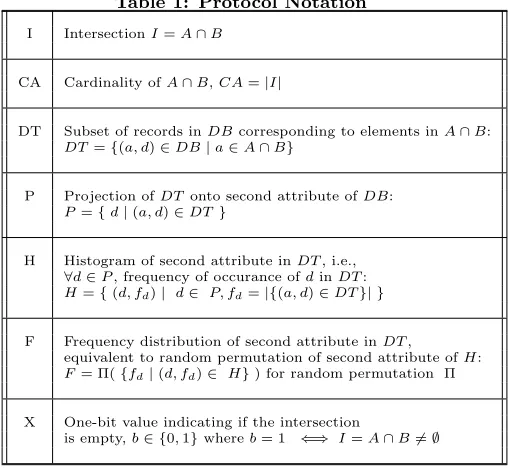
In every PSI protocol flavor, Server’s input consists of a two-attribute database (table)DB={(a1, d1), . . . ,(an, dn)} where the set of first attributes is A ={a1, . . . , an}, and Client’s input is a set: B ={b1, . . . , bm}. At the end of a protocol,Clientlearns some of the following information, shown in Table 1.
For a subsetL ⊂ {I, DT, P, H, F, CA, X}we now define PSI-L to be a protocol wherein Client learns nothing be-yond information indicated byLand |A|. This notation is reflected in Table 1. For its part,Serverlearns nothing ex-cept|B|. Armed with this notation, we now define a family of PSI protocols.
Definition 1 (PSI-L). LetL ⊂ {I,DT,P,H,F,CA,X}. PSI-L is a two-party protocol involving Server and Client. Server input consists ofDB={(a1, d1), . . . ,(an, dn)}where the first attribute representsA={a1, . . . , an}. Client input is a set of elements: B={b1, . . . , bm}. At the end of execu-tion, Client outputs the information specified inLand |C|
and Server outputs|B|. No party learns any further infor-mation.
Table 1: Protocol Notation
I IntersectionI=A∩B
CA Cardinality ofA∩B,CA=|I|
DT Subset of records inDBcorresponding to elements inA∩B:
DT={(a, d)∈DB|a∈A∩B}
P Projection ofDT onto second attribute ofDB:
P={d|(a, d)∈DT}
H Histogram of second attribute inDT, i.e.,
∀d∈P, frequency of occurance ofdinDT:
H={(d, fd)| d∈ P, fd=|{(a, d)∈DT}| }
F Frequency distribution of second attribute inDT,
equivalent to random permutation of second attribute ofH:
F= Π({fd|(d, fd)∈ H}) for random permutation Π
X One-bit value indicating if the intersection
is empty,b∈ {0,1}whereb= 1 ⇐⇒ I=A∩B6=∅
We denote a given Lvariant by appending its symbol to the string “PSI”, e.g., for L ={P, H}we write PSI-Las PSI-P-H. We now make some observations on this notation and relationships among protocol variants, summarized in Figure 1.
DT
I H
F
CA P
X
Figure 1: Relationships between information dis-closed by various PSI protocols.
• Standard PSI protocols that compute the set intersec-tionA∩B are called PSI-I in our notation.
• Our notions of PSI-CA and PSI-DT coincide with their common prior use in the literature.
• Our representation is not unique, e.g., PSI-DT can also be written as PSI-DT-I-P-H.
• Notation X → Y means: “knowledge of X implies knowledge ofY”.
• PSI-DT discloses the maximum amount of information among all protocols in this family.
the first two by removing any linkage between elements in
P and their frequencies, i.e., we progress from a protocol disclosing H to a protocol disclosing F and P. In Section 4, we remove knowledge of F fromClientand construct a PSI-P protocol. This is the hardest step. The key building block for a PSI-P protocol is a sub-protocol for PSI-X.
2.2
Privacy Advantages of Projection Variants
Before proceeding to concrete protocols, we consider de-grees of privacy attainable with various envisaged PSI-based projection techniques, compared to PSI-DT.2.2.1
PSI-P
Recall that m and n are respective sizes of Client and
Server inputs. From the privacy perspective, in an ideal PSI-P protocol,Clientlearns only:
P ={di| ∃(ai∈A, bj∈B)3bj=ai}
However, in some extreme cases, PSI-P offers no privacy over PSI-DT. For example, if w=|P|= 0, thenA∩B = ∅ and no additional information is learned in either pro-tocol. Also, if m = 1, then w ∈ {0,1} and both PSI-P and PSI-PSI-DT yield equivalent knowledge. Nonetheless, in general, PSI-P that results in Client learning P offers more privacy toServerthan PSI-DT which letsClientlearn N={(ai, di)∈A| ∃(bj∈B)3bj=ai}. In other words, PSI-P offers no privacy over PSI-PSI-DT if m= 1 or w = 0. The same is true whenw=m.
Aside from these corner cases, PSI-P can offer a signif-icant privacy advantage over PSI-DT. In general, we can express the number of possible mappings of elements in B to elements in P as:
MP(m, w) =
( m+ 1
w+ 1
)
·w! (1)
wheren
k represents the Stirling number of the second kind, i.e., the number of ways to partitionn objects into k non-empty subsets. Eq. (1) is the number of partial surjective functions fromB to P. The mappings are partial because some elements inB might not be in A∩B, and surjective because each element in P has at least one corresponding element inB. LetMT(m, w) be the number oftotal surjec-tive functions fromB toP. This is known to be: m
w ·w!; see for instance the twelve-fold way [26]. For each non-total functionf, let f0 :B →P∪ {}wheref0(x) =for every
x undefined through f. The number of such functions is MT(m, w+ 1). Adding to this number the partial functions that are already summed up gives:
MT(m, w+ 1) +MT(m, w) =
n m
w+ 1
o
·(w+ 1)! +
nm w o
·w!
=MP(m, w)
by the recurrence relation of Stirling numbers of the second kindn+1
k =k
n
k +
n
k−1 . This expression also assumes (perhaps idealistically) thatClienthas no extra information about DB and its second attribute is uniformly distributed. GivenMP(m, w), we can capture the exact degree of pri-vacy (Dpriv) that PSI-P offers over PSI-DT as:
Dpriv= 1− 1 MP(m, w)
As reflected by aforementioned “corner cases”, Dpriv = 0 for m = 1 or w = 0. We also note that perfect privacy
(Dpriv = 1) is unattainable form ≥1. Indeed, Dpriv = 1 only ifm= 0, i.e,B=∅.
2.2.2
PSI-P-H
PSI-P-H allowsClientto learn the histogramH (see Ta-ble 1) which also leaks CA=|A∩B|. It thus yields more information than P given by PSI-P, though less information than N given by PSI-DT.
Let MH(m, w, H) be the number of possible mappings from elements in B={b1, . . . , bm} to elements in P, given projection histogram H. Letfi relate to the frequency of the i-th element in P, that is such that (Pi, fi)∈H. The number of such mappings is the product of the number of ways to choose f1 elements among m and the number of ways to choosef2 elements amongm−f1, etc. That is:
MH(m, w, H) = w
Y
k=1
m−Pk−1 i=1fi
fk
!
= w
Y
k=1
(m−Pk−1 i=1fi)!
fk!(m−Pki=1fi)!
= m!
Qw k=1fk!
(m−Pk i=1fi)! Note that this number does not rely on the order in which projection elements are considered.
2.2.3
PSI-P-F
PSI-P-F allowsClient to learn P and F, both of size w
(see Table 1). It thus offers more privacy than PSI-P-H, over PSI-DT. The number of mappings from elements in B={b1, . . . , bm} to projection set elements, given the ran-domly permuted projection histogramF, is:
MF(m, w, F) =MH(m, w, H)·πF,
with πF the number of possible histograms related to F. That is, the number of permutations with repetition of in-distinguishable objects:
πF =
w!
Q ni!
withni=|{i∈F}|, the number of occurences of a frequency
iinF. For example, withm= 8, w= 4, H= (1,3,1,1), we have:
• MH(8,4,(1,3,1,1)) = 3!2!8! = 6720 • MF(8,4,(1,1,1,3)) = 6720·4!3!= 26880 • MP(8,4) = 6951·4! = 166824
In the corner case, whenm=w, andF=H= (1,1, . . . ,1), we have: MF(m, w, F) = MH(m, w, H) = MP(m, w) =
m!. Finally, note that the same measure of privacy Dpriv defined for PSI-P can be used for PSI-P-H and PSI-P-F, since in each case all mappings are equally likely.
3.
PROTOCOLS
We now proceed to construct a series of protocols with variable degrees of privacy, falling into the range between PSI-DT and PSI-P.
3.1
Initial PSI-P-H Protocol
section. We can achieve this easily by modifying any OPE-based3PSI protocol (e.g., [14]), as described below.
Setup: ServerandClientrespective inputs are:
DB = {(a1, d1), . . . ,(an, dn)} and B = {b1, . . . , bm}, re-spectively. A={a1, . . . , an}is the first attribute ofDB = {(a1, d1), . . . ,(an, dn)}. Let E be an additively homomor-phic encryption scheme, e.g., Paillier [24], andEncbe a sym-metric authenticated encryption scheme (AKE), e.g., [2].
1. Client generates a new public/secret key-pair for E.
Client encodes each element from B = {b1, . . . , bm} as a root of a polynomialP :=Qm
i=1(X−bi). Next, Clientencrypts the coefficients ofP usingEand sends the resulting list of encrypted coefficients to Server, together with the new public key.
2. For each ai ∈ A = {a1, . . . , an}, Server chooses, at random, symmetric key ki and identifier oi. It then computesqi:=Encki(di) and formsQ={q1, . . . , qn}. 3. For each (ai, di)∈DB,ServercomputesE(ri·P(ai) +
kikoi), withrirandom numbers, using the homomor-phic properties ofE and adds resulting elements to a list L. Server shufflesLandQand sends the shuffled sets toClient.
4. Client decrypts elements in L and parses the result intokko. If there is an element inQmarkedo,Client
decrypts it withk. If the integrity check holds,Client
obtainsd. Otherwise,Clientdiscards this element. Because of an AKE scheme,Clientcan distinguish whether decryption of qi in Step 4 is a random value or an actual attribute (that it needs to learn) associated with an element inA∩B.
Computation cost is dominated by O(nm) exponentia-tions, if we use the Paillier scheme. By applying Horner’s rule and binning techniques we can reduce computation to
O(nlog log(m)) exponentiations [14].
In this protocol, Client learns the histogram H without learning A∩B. Recall that our ultimate goal is to hide the frequencies, or equivalently, to deduplicate the projec-tion. However, this seems difficult in protocols that work “point-by-point”, such as the one above. For example, if
A = {a1, a2} and DB = {(a1, d1),(a2, d1)}, Client learns two independent outputs that could yield further informa-tion, depending on B. What is missing is the ability to
aggregate two independent outputs, such that the cases of |A∩B|= 1 and|A∩B|= 2 are indistinguishable toClient. This illustrates a basic limitation of such “point-by-point” protocols in attaining PSI-P with maximal privacy. In con-trast, protocols in Section 4 below provide this kind of ag-gregation capability.
3.2
A More Practical PSI-P-H Protocol
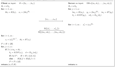
We now present a PSI-P-H protocol with a linear com-putation cost, which is much more efficient than the ini-tial protocol. The intuition is to modify the basic PSI-CA protocol from [7]4 to perform data transfer with techniques similar to traditional OPRF-based PSI-DT protocols, such as [20]. Specifically, as in PSI-CA,ClientandServer evalu-ate an Oblivious Pseudo-Random Function (OPRF) on each of Client’s set elements. Then, for every record in DB,3
OPE: Oblivious Polynomial Evaluation.
4Note that in [7], the protocol contains an additional DH-like key exchange that was subsequently removed in the latest version [8]. Private communication with the authors clari-fied that this key exchange is not required.
Server transfers its second-attribute value encrypted under a unique key derived from the pre-image of the OPRF eval-uated over the value of the first attribute of the same record. This way,Clientonly decrypts second-attribute values (di-s) that correspond to elements in the intersection.
This protocol needs a semantically secure symmetric-key encryption function (Ek(·), Dk(·)), a corresponding key deriva-tion funcderiva-tionKDF(·), two random oraclesH(·)5 andH0(·),
random permutation Π(·), and a keyed pseudorandom func-tionFk(x) =H0(gkH(x)), based on the following group pa-rameters: primespandq (wherep= 2ql+ 1) and a gener-atorg of order q in a subgroup ofZp. The resulting PSI-P-H protocol is shown in Figure 2. The notation is largely self-explanatory, except for H[d] which denotes an element (d, f) ∈ H where d is a data item andf is its frequency up to now. H[d].f denotes the frequency attribute/field of element (d, f).
On its own, this protocol comes very close to the desired PSI-P functionality. Unfortunately, it does not address the deduplication problem. At the same time, for some applica-tions where this information leakage is acceptable or desired, this is the most efficient protocol that we identified thus far. It is also easy to see that this protocol, being a minor vari-ation of the original PSI-CA, leaks no informvari-ation beyond the histogram, assuming that all encrypted data valuesedj are of uniform size. See Section 3.6 for more details.
3.3
PSI-DT with Deduplication
The main challenge in constructing an ideal PSI-P pro-tocol is how to handle data deduplication to avoid privacy leakage. Another issue is bandwidth: ideally, the protocol should transfer associated data values (corresponding to the intersection computed on the first attribute) only once. This is particularly the case if these values are large, e.g., photos or video clips. We now present a trick for reducing privacy leakage from frequencies, and also lowering bandwidth con-sumption.
We construct a protocol based on two rounds of PSI-DT. First, we introduce a randomly generated tag,tk←${0,1}`,
for each unique data valuedk. This producesDBA, a map-ping betweenAand randomly generated tags, where distinct elements inAmapping to the same data value inDBare as-sociated with the same tag inDBA. Another data structure
DBTmaps distinct tags to data values.
Then,ClientandServerrun PSI-DT on these (potentially duplicated) tags instead of data values. Note that while the number of tags and distinct data values is the same, the size of the former is uniform and may be significantly smaller.
Next, Client filters all duplicate tags and then pads the resulting set of tags with randomly generated tags, up to the size of min(m, n). This is necessary to precludeServer
from learning CA. Alghough padding incurs additional com-putation in PSI-P-H, dummy tags need not be blinded by
Client; they should only be indistinguishable from actual blinded elements.
Then,Client runs PSI-DT for the second time, its input being the deduplicated padded set of unique tags. Server
input in this round includes the tags and their mapping to data items. This way,Serveronly sends each encrypted data item once, regardless of the number of set elements which map to it. Details are shown in Figure 9 in Appendix A.
PSI-P-Hon input:H(·),H0(·),p,g,Ek(·),Dk(·),KDF(·)
Clienton input: B={b1, . . . , bm} Serveron input: DB={(a1, d1), . . . ,(an, dn)}
Rc←$Zq Rs←$Zq
fori= 1..m: forj= 1..n:
hbi=H(bi), xi= (hbi)Rc haj=H(aj), yj= (haj)Rs, taj=H0(yj)
kj=KDF(yj), edj=Ekj(dj)
{x1, . . . , xm}
fori= 1..m: x0i= (xi)Rs
Π(
x01, . . . , x0m )
Π({(ta1, ed1), . . . ,(tan, edn)})
fori= 1..m:
zi= (x0i)R −1
c , tbi=H0(zi)
P=H={∅} forj= 1..n:
if∃i3taj=tbi:
kj=KDF(zi), d=Dkj(edj)
ifd6∈P: H=H∪ {(d,1)} else : H[d].f=H[d].f+ 1
P=P∪ {d}
return(n, P, H) returnm
Figure 2: PSI with Projection and Histogram (PSI-P-H). All computation is modp, unless otherwise stated.
At the end of the protocolClient learns the same infor-mation as in PSI-DT, in particular, the histogramH. How-ever, each encrypted data item is only transferred once, in the second round. If data items are large this can result in appreciable bandwidth savings. However, these savings come at increased computation by a factor of at most 2, since PSI-DT is run twice.
Also, Client learns k – the number of distinct data ele-ments in DB. This can be avoided (see 3.5) at the cost of negating bandwidth savings. Indeed, disclosure of k is inherent to each data element being sent only once.
3.4
Practical PSI-P-F Protocol
In our previous protocolsClientlearnsH – the histogram of data items in projection N. We now show how to construct an efficient (lintime) PSI-P-F protocol. As argued ear-lier, disclosing only the frequencies toClient(and not their linkage to elements in the projection set) is a major practical privacy gain.
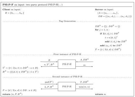
To construct a practical PSI-P-F protocol, we use the deduplication technique described in Section 3.3 and re-flected in Figure 9), except, instead of PSI-DT, we run PSI-P-H twice. The resulting protocol is a practical, linear-time instantiation of PSI-P-F. Its offers better privacy since
Client only learns the histogram of tags in the first exe-cution of PSI-P-H. The second exeexe-cution of PSI-P-H re-moves the mapping between tags and second-attribute val-ues, thereby also removing any association between frequen-cies and second-attribute values. The protocol is shown in Figure 3.
Note that, as with PSI-DT with deduplication, Client
learns k – the number of distinct second-attribute values inDB. This is not the case in PSI-P-H from Section 3.2. See Section 3.5 for a discussion.
3.5
Hiding Number of Distinct Data Elements
The number of distinct data elementsk =|{d |(a, d) ∈DB}| is revealed in both PSI-DT with deduplication and PSI-P-F. This is inherent to transmitting each (encrypted) data element (aka second-attribute value) only once. This leakage in P-H can be avoided by running a simple PSI-DT protocol; however the sole advantage of PSI-PSI-DT with deduplication over PSI-DT is bandwidth savings.
In PSI-P-F, leakage can be avoided by havingServerpad
DBT ton ≥k pairs, using random tags (indistinguishable from real tags byClient) and dummy enryptions. Although this would result in no bandwitdh savings, it might be useful in scenarios where data elements are small and/or privacy ofkis important.
Given that this leakage can be avoided, it is omitted from the final output of PSI-DT with deduplication as well as PSI-P-F in Section 3.6. Finally, this leakage is absent in PSI-P presented later in Section 4.
3.6
Correctness & Privacy
Definition 2 (Correctness of PSI-L). If both par-ties are honest, at the end of protocol execution on respective inputs[(B),(A, DB)], Client outputs(n,L)and Server out-putsm.
PSI-P-Fon input: two party protocol PSI-P-H(·,·)
Clienton input: Serveron input:
B={b1, . . . , bm} (A={a1, . . . , an},
DB={(a1, d1), . . . ,(an, dn)})
. . . Tag Generation . . . .
DBA={}; DBT={} forj= 1..n:
if@(t, dj)∈DBT t←${0,1}`
add(t, dj)toDBT
add(aj, t)toDBA T={t| ∃(t, d)∈DBT}
. . . First instance of PSI-P-H . . . .
T0={t| ∃(a, t)∈DBA:a∈B}
PSI-P-H
B A, DBA
n, T0, HA
m
HA= (|{(d, t)∈DBA}| |t∈T0)
. . . Second instance of PSI-P-H . . . .
P={d| ∃(a, d)∈DB:a∈B}
PSI-P-H
pad(T0) T , DBT
k, P, HT min(m, n)
return(n, P, HA) returnm
Figure 3: PSI with Projection and Frequency distribution (PSI-P-F).
[(B),(A, DB)], Client learns nothing beyond(n,L)and Server learns nothing beyondm.
Theorem 1. PSI-P-H is correct.
Proof. We have: zi=x 0R−c1
i =x
Rs/Rc πi =hb
Rs
πi for some 1 ≤πi ≤ m (corresponding element in the first permuta-tion). Doing the same foryj, we express:
tbi=H 0
(zi) =H 0
(hbRsπi) and taj=H 0
(yj) =H 0
(haRsj )
For indicesj, such that tbi=taj for some 1≤i≤m, the above equations imply thatbπi =aj and alsozi=yj. The corresponding elementedj is decrypted using a key derived from yj = zi. Note that H is deduced from this process becauseClientlearns the number oftaj-s associated with a given data item in projection.
Theorem 2. PSI-P-F is correct.
Proof. In the first instance of PSI-P-H,ClientlearnsT0
– tags associated with items in the intersection and their histogram (by Theorem 1). Therefore, F (randomized his-togram of corresponding data items). In the second PSI-P-H,Clientlearns data items associated with tag elements, i.e., PSI-P.Clientalso learns their histogramHT(again, by Theorem 1). However, each data item is mapped only to one tag inDBT; thus, no additional information is leaked.
Our P-H construction is substantially based on the PSI-CA technique from [7]. The argument for its privacy is there-fore very similar, and relies on the very same assumptions,
i.e., semi-honest (HbC) participants, DDH, One-More-DH, and Gap-One-More-DH assumptions; we refer to [7] for fur-ther details.
Theorem 3. PSI-P-H is private.
Proof (Sketch). Server privacy: The main addition of PSI-P-H over PSI-CA is that, inServer’s reply, encrypted data elements are associated with hashed blinded elements.
Client can not learn anything from encrypted elements for which it does not know the decryption keys, based on secu-rity of E(·. Ah decryption key can be learned only if the corresponding element is in the intersection.
Clientprivacy:Serverlearns nothing more than in PSI-CA, which is private.
Theorem 4. PSI-P-F is private.
Proof (Sketch). Server privacy: Based on the
defini-tion of PSI-P-H and its privacy (Theorem 3),Clientlearns P and H related toBandDBA, and (padded)T0andDBT, respectively.
In the first exchange, this reveals (fromDBA) tags mapped to items inA∩Band their histogram. Nothing is learnt from tag values since they are selected at random. Even though the histogram HA leaks frequency distribution of tags, it conveys no information about the histogram of data items, since their order is randomly permuted.
It is computationally infeasible forClient to learn the tags corresponding to items outside the intersection and learn additional data items.
ClientprivacyServerlearns nothing beyondmfrom either interaction (by Theorem 3). In particular, in the second exchange, sinceClientinput is padded to min(m, n),Server
can not learn CA. It also can not distinguish its own tags from padding tags generated by Client, since all tags are blinded by the latter.
4.
PSI-P & PSI-X: HIDING FREQUENCIES
Our strategy in this paper is to progress from a PSI-DT (=PSI-DT-I-P-H-F) protocol to a PSI-P protocol by remov-ing information fromClient’s output. In the previous sec-tion, we constructed a very efficient and practical PSI-P-F protocol that builds upon some prior PSI constructions. In this section we aim to hide the frequencies (F) fromClient. As mentioned in the discussion of the OPE-based PSI-P-H protocol, in order to hide frequencies, we need the ability to aggregate responses that result from comparing elementsai∈A={a1, . . . , an}withbj∈B ={b1, . . . , bm}. Given a fully homomorphic encryption (FHE) scheme, aggregation on (encrypted) responses is possible. Furthermore, PSI-X is also easily attainable with FHE. One na¨ıve way to do so (albeit with quadratic complexity) is to compute: (1)
yij = E(rij∗(ai−bj)) for each i ∈ [1, n], j ∈ [1, m] and unique random rij, and then: (2) E(Qn,mi=1,j=1(yij)). The result of (2) would decrypt to zero iffA∩B 6=∅and to a random value, otherwise.
However, with only an additively homomorphic encryp-tion (AHE) scheme such as Pailler, as in the OPE setting, there is no obvious way to do that. Unfortunately FHE is not yet practical. To this end, we present a new alterna-tive construction that offers aggregation without FHE. The protocols achieve PSI-P and PSI-X. However they are more expensive than techniques presented in Section 3.4.
4.1
PSI-X Construction
In the simplest situation for aggregation (or deduplica-tion) there is only one distinct second-attribute value.Server
input is DB={(a1, d1), . . . ,(an, dn)}where d1 =d2 =...=
dn, whileClientinput is B={b1, . . . , bm}. Clientshould learn
d1iffA∩B6=∅, otherwiseClientlearns nothing other than
A∩B=∅. This is very similar to PSI-X whereClientlearns 1 ifA∩B6=∅and 0 otherwise.
The first step to construct a protocol for PSI-X is to rep-resent the setsAandBby their characteristic functionsχA andχB. Comparison of individual elements at positioniis given by the productχA(i)χB(i). Their aggregation is the disjunction:
_
∀i
χA(i)χB(i) (2)
which is 1 iffA∩B6=∅.
We can evaluate this Boolean formula in Eq. (2) on en-crypted values using, for example, Boneh-Goh-Nissim (BGN) [3] partially homomorphic encryption scheme, which allows multiply-once/add-many homomorphic operations. More precisely, BGN can be used to evaluate 2-DNF formulas on cipher-text.
However, in general, the size ofU, the universe the set ele-ments belong to, is either not bounded or too big for storing the characteristic functions efficiently. Instead, we store the
characteristic functions in a lossy manner, by choosing a random 2-universal hash-function h : U → [1, . . . , N] (for appropriately chosenN) [5] and applying it to the sets. We then check whetherh(A)∩h(B)6=∅by evaluating the for-mula in Eq. (2) for h(A) and h(B). This introduces the possibility of false positives due to hash collisions. A false positive occurs when A∩B =∅ while h(A)∩ h(B) 6=∅. It is easy to see that this error probability is a constantP
that depends only on the parameters of the protocols (P is computed below). In other words, it depends on n, m, N, and not on the specific A and B. If A∩B 6= ∅ then
h(A)∩h(B)6=∅and Eq. (2) always yields a correct answer. We can lower the error probability exponentially through a series of independent rounds.
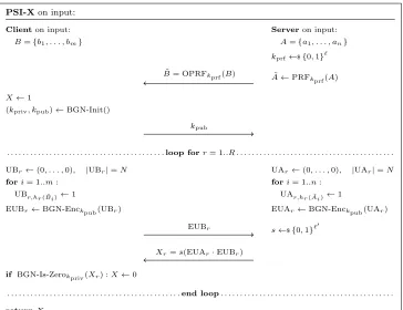
The protocol is depicted in Figure 4. First,Ais blinded using a keyed PRF andBis blinded using an oblivious evalu-ation of that PRF (OPRF) under the same key. The reason for the oblivious evaluation is to provide forward security.
Client then initializes a BGN key-pair and transmits the public key to the server. Then, the following procedure is repeatedRtimes.
A 2-universal hash function h : U → [1, . . . , N] is ran-domly chosen by both parties from a fmaily of hash function H(see more detail below about optimally choosingN). Bit vector UA (and likewise for UB) of size N are built for A
such that UAi = 1 ⇐⇒ ∃x∈A˜:h(x) =i. Both vectors are encrypted under BGN byServerandClient respectively.
Clientsends its set toServer, who evaluates Eq. (2) on en-crypted values. Server picks a randoms to randomize the intermediate result using the scheme’s homomorphic prop-erties (as in the basic protocol in [3]) and sends the result back. Client tests if the received value is an encryption of 0. If yes, the intersection is guaranteed to be empty. Oth-erwise, either the intersection is non-empty or a false pos-itive occurred with probabilityP as outlined above. After
Rrounds,Clientderives the output of PSI-X. IfA∩B6=∅, the output is always 1 – the correct answer. If A∩B =∅, the output is 0, which is correct with probability 1−PR.
We now have
Theorem 5. PSI-X is a randomized algorithm with a one-sided error. For input setsAandBwithA∩B6=∅the algo-rithm always answers correctly. IfA∩B=∅the algorithm answers correctly with probability1−PR, where
P = 1−
1− 1
N mn
≈1−e−mn/N
andRis the number of rounds. ForN=log 2mn andmnlarge we haveP ≈1/2.
In this theorem and in what follows, log denotes the nat-ural logarithm. The proof follows from the discussion above and the fact that for any given distinct valuesx, y∈U and for a family H = {h : U → [1, ...N]} of 2-universal hash functions we have Prh∈H[h(x) =h(y)] = 1/N.
PSI-Xon input:
Clienton input: Serveron input:
B={b1, . . . , bm} A={a1, . . . , an}
kprf←${0,1}`
˜
B= OPRFkprf(B) A˜←PRFkprf(A)
X←1
(kpriv, kpub)←BGN-Init()
kpub
. . . .loop forr= 1..R. . . .
UBr←(0, . . . ,0), |UBr|=N UAr←(0, . . . ,0), |UAr|=N
fori= 1..m: fori= 1..n:
UBr,hr( ˜Bi)←1 UAr,hr( ˜Ai)←1
EUBr←BGN-Enckpub(UBr) EUAr←BGN-Enckpub(UAr)
EUBr s←${0,1}`0
Xr=s(EUAr·EUBr)
if BGN-Is-Zerokpriv(Xr) :X←0
. . . .end loop. . . .
returnX
Figure 4: Existential PSI (PSI-X).
Theorem 6. The number of ciphertext multiplication op-erationsCX in PSI-X is minimized when
N = mn log 2,
giving
CX=−
mnlogPX log22 ,
for a desired total probability of false positivePX. For this choice ofN the number of rounds isR= logPX
logP , withP the probability of a false positive in one round.
Proof. See Appendix B
We now show PSI-X has the desired privacy properties. PSI-X uses as subprotocols an OPRF protocol [15, 19] and the SFE protocol for evaluating 2-DNF formulas from [3]. The 2-DNF protocol is secure under the Subgroup Decision Assumption.
Theorem 7. Given a secure OPRF protocol and under the Subgroup Decision Assumption PSI-X is private.
Proof (Sketch). PSI-X has three steps. First Client
and Server engage in an OPRF protocol. Second there is a hashing step with a randomly chosen 2-universal hash func-tionh. Third there is a secure evaluation of a 2-DNF formula Eq. (2) on the outputs from the hashing step. Hashing and 2-DNF formula evaluation are repeated in R independent rounds.
Client privacyThe OPRF protocol does not leak infor-mation to the Server about Client’s input due to its pri-vacy guarantees. In Step 3 Server additionally receives a
set of BGN-encrypted values from Client. Under the Sub-group Decision Assumption BGN encryption is semantically secure and thus Server does not learn anything from these ciphertexts.
Server privacyWe show that a simulatorC∗can simu-late the Client’s view of the protocol from its input and the protocol output. The Client’s view consists of OPRF(B), i.e. OPRF applied to his input B. In the i’th round of the protocol Client sees a randomly chosen 2-universal hash function hi, the result from the secure evaluation of the 2-DNF formula applied tohi(OP RF(B)) and the binary out-putoi:= BGN-Is-Zerokpriv(Xr) of the 2-DNF computation.
If the PSI-X protocol outputs 1 then all theoihave been 1 by definition of the protocol. In the simulationC∗generates a set of random values in the range of the PRF. This set is indistinguishable from the set OPRF(B) without knowledge ofkprf. In addition he sets each bit in bit vector UA to be 1 at every location, and then proceeds as would the Server sending backXi=s(EUAi·EUBi). This ensuresoi= 1 for alli. Using sequential composition theorems for multiparty computation we can assume that the OPRF protocol and the secure 2-DNF evaluation protocol are given as in the ideal model. This simulation is indistinguishable from the execution of the real protocol.
pro-tocol and the secure 2-DNF evaluation propro-tocol are given as in the ideal model. This simulation is computationally indistinguishable from the Client’s view of the real PSI-X protocol execution.
4.2
Full PSI-P Protocol
The main idea is to use PSI-X to determine, for each sec-ond attribute valuedi, whether the elements inAthat map to each second attribute valuediintersect withB. Such ele-ments of the second attribute are then transferred toClient
using PSI-DT. The full protocol is depicted in Fig. 5 and described below.
LetD={di|(ai, di)∈DB}denote a set of distinct second-value attribute second-values, such that |D| = k ≤ n. Let de-note a dummy value. Server first builds a vector V com-prised of elements ofD, padded withn−k dummy values, such that|V|= n, and then shuffles it. For each d = Vi, Servercomputes its support, defined as: support(d) ={ai∈
A| (ai, di) ∈ DB}, with support() = ∅. Then, support is padded such that the size of the ensuing vector isn. The padding scheme pad(·) that we suggest is to use elements from a subset of U disjoint from the possible values in A
andBand agreed upon by ClientandServer. Next,Client
andServer engage in a PSI-X protocol with respective in-putsB and pad(support(Vi))). After this is done for each element of V,Client and Server engage in a final PSI-DT protocol for the elements ofV that resulted in PSI-X output 1.
False positives in PSI-X executions result in elements of
D being incorrectly transferred. This can be alleviated by tuning the number of rounds in PSI-X.
Theorem 8. Let Server’s input beDB={(a1, d1), . . . ,(an, dn)} and Client’s input be B = {b1, . . . , bm}. PSI-P is a ran-domized algorithm so that at the end of the protocol Client learns a setP rsuch thatP r⊃ {di| ∃(i, j)3bj=ai}. With probability at least1−nPR equality holds, i.e. P r={d
i | ∃(i, j) 3bj =ai}, where PR is the error probability of the PSI-X sub-protocol.
The proof follows directly from the prior discussion and Theorem 5.
PSI-P uses as subroutines PSI-X and PSI-DT. It now fol-lows from Theorem 7
Theorem 9. Given a secure OPRF protocol, a private PSI-DT protocol and under the Subgroup Decision Assump-tion, PSI-P privately computesP r⊃ {di| ∃(i, j)3bj=ai}. With probability at least 1−nPR, no additional element beyond the actual projection is revealed, i.e. P r = {di | ∃(i, j) 3bj =ai}, where PR is the error probability of the PSI-X sub-protocol.
There aren executions of PSI-X with sets of sizemand
nand one execution of PSI-DT with a set of sizen.
Theorem 10. The number of ciphertext multiplication op-erationsCP is given by
CP≈
mn2loglog 1−−nP
P
log22 +CDT(n)∈ O
mn2log n −log 1−PP
,
for a desired total probability of false positive PP, and with
CDT the cost of the PSI-DT execution.
Proof. See Appendix B
Although considerably more expensive than the construc-tion given in Sect. 3.4, PSI-P protects privacy of bothServer
andClientand does not disclose any other information than the projection.
Some elements in its construction help achieve that. Firstly, there are n rounds of PSI-X instead of k (although n−k
of these rounds are dummy rounds) so that client does not learnk, the number of different data elements. Additionally, the support of (possibly dummy) data elements are padded to sets of sizenso that client does not learn the histogram of data items. Finally, the data transfer operation is done after thenrounds of PSI-X so as to not give information on the server about the result of the individual PSI-X executions.
5.
EXPERIMENTS
5.1
PSI-P-H and PSI-P-F
We implemented PSI-P-H (Fig. 2) and PSI-P-F (Fig. 3) in order to have a practical measure of their efficiency. We used a custom fast implementation of PSI-DT that uses OPRF as a building block for PSI-P-F. Experiments were run on an Intel i7-4710HQ CPU.
Figures 6, 7, and 8 represent the cost of PSI-P-H and PSI-P-F for different values ofmandn= 100 for when the intersectionA∩B is respectively empty, half the size ofB, and the entire setB. The overhead of PSI-P-F with respect to H corresponds to the second instance of PSI-P-H within PSI-P-F. This second instance has a small fixed cost, and depends linearly on the size of the intersection. For PSI-P-H however, the size of the intersection does not matter.
0 20 40 60 80 100
m 0
100 200 300 400 500 600
time [ms]
PSI-P-H PSI-P-F
Figure 6: Comparison of the cost of PSI-P-H and PSI-P-F for varyingm withn= 100 and|A∩B|= 0.
5.2
PSI-P
For PSI-X (Fig. 4) and PSI-P (Fig. 5), we used Relic [1], an efficient library in C for cryptographic protocols. It is used notably for the BGN encryption scheme in PSI-X. PSI-P also uses our OPRF-based PSI-DT implementation. Exper-iments are again run on an Intel i7-4710HQ CPU.
PSI-Pon input:
Clienton input: Serveron input:
B={b1, . . . , bm} (A={a1, . . . , an},
DB={(a1, d1), . . . ,(an, dn)}) D={d| ∃a∈A: (a, d)∈DB} |D|=k≤n
V ←shuffle(D1, . . . , Dk, , . . . ,
| {z }
n−k
)
. . . .loop fori= 1..n. . . .
Xi= PSI-X(B,pad(support(Vi)))
. . . .end loop. . . .
I← {i|Xi= 1}
P= PSI-DT(I,{1, . . . , n}, V)
returnP
Figure 5: PSI with Projection (PSI-P).
0 20 40 60 80 100
m 0
100 200 300 400 500 600 700 800
time [ms]
PSI-P-H PSI-P-F
Figure 7: Comparison of the cost of PSI-P-H and PSI-P-F for varyingmwithn= 100and|A∩B|=m/2.
0 20 40 60 80 100
m 0
100 200 300 400 500 600 700 800 900
time [ms]
PSI-P-H PSI-P-F
Figure 8: Comparison of the cost of PSI-P-H and PSI-P-F for varyingmwithn= 100 and|A∩B|=m.
but this has no impact on the protocol efficiency (otherwise this would constitute a leakage of CA). “BGN dot prod-uct” corresponds to the EUAr·EUBr operation in Fig. 4.
“Other BGN” corresponds to BGN encryptions, decryptions, and initialization in PSI-X. “PSI-DT” is the final operation in PSI-P. Time reported are aggregated for the Client and
Server, butServerdoes most of the work, since it computes the BGN dot products.
6.
PSI-P WITH THRESHOLD CONDITIONS
In some scenarios it will be useful to transfer the addi-tional item d only if there has been a match of Client’s input B={b1, . . . , bm} for at leasttelements with Server’s input A={a1, . . . , an}for a thresholdt. For exampleAmay contain 300 domain names which are associated with a par-ticular attack campaign. Although connecting with one do-main inA may be inconclusive, if there were more than 20 connections from theClient’s network this might be strong evidence that an intrusion took place and consequently that additional datadshould be sent toClient.
Our framework can handle threshold conditions naturally by applying at-out-of-nShamir secret sharing scheme tod. For each matching indicator, using PSI-P-H, a (different) share of d is transferred to Client. Client can then recon-structdif and only if he learned at leasttshares.
This yields a practical threshold scheme for (1) transfer-ring additional data if and only a threshold condition is met and (2) not revealing the matching indicators themselves. The privacy guarantees of this solution are likely sufficient in many practical scenarios.
However there is still some information leakage. In addi-tion tod(the only dataClientshould learn if conditions are met),Clientalso learns thresholdtand how many shares for reconstructingdhe actually received (which could be more than t). We believe the question how to reduce informa-tion leakage in threshold scenarios is an interesting, open problem for future work.
7.
RELATED WORK
oblivi-Table 2: Times (in seconds) of different parts of the PSI-P protocol.
n m Total time BGN dot product Other BGN PSI-DT Remaining operations
3 3 3.05 2.29 (75.01%) 0.67 (21.86%) 0.10 (3.12%) 0.00 (<0.01%)
5 5 13.79 11.33 (82.20%) 2.35 (17.08%) 0.10 (0.72%) 0.00 (<0.01%)
10 10 107.43 91.35 (85.04%) 15.96 (14.85%) 0.12 (0.11%) 0.00 (<0.01%)
20 20 843.76 722.90 (85.68%) 120.74 (14.31%) 0.12 (0.01%) 0.00 (<0.01%)
5 20 53.45 45.41 (84.97%) 7.88 (14.74%) 0.16 (0.29%) 0.00 (<0.01%)
20 5 211.56 179.96 (85.06%) 31.53 (14.91%) 0.07 (0.03%) 0.00 (<0.01%)
ous polynomial evaluation (OPE). Kissner & Song [22] soon thereafter proposed another set of somewhat more efficient PSI-like OPE-based protocols, applicable to 2-part as well as larger group settings, i.e., more than justClientandServer. Jarecki & Liu [19], Hazay & Lindell [15] and De Cristofaro & Tsudik [10] each proposed various efficient linear-complexity OPRF-based PSI techniques secure in the Honest-but-Curious (HbC) adversary model. Dachman-Soled et al. [6] Hazay & Nissim [16], and De Cristofaro et al. [9] constructed (rel-atively efficient) PSI protocols secure in the malicious ad-versary model. Huang et al. [18] designed a PSI protocol based on garbled circuits, which is allegedly faster than the fastest OPRF-based PSI protocols, at least for a high secu-rity parameter. These claims have been since disputed in [11]. There also several PSI protocols based on Bloom Fil-ters, such as [13, 21, 23]. We do not consider them due to extra information leakage as far as false positives.
Several PSI-CA protocols have been proposed thus far. The PSI protocol in [14] can be extended to PSI-CA with similar complexity. [17] presents a PSI-CA protocol based on [14] with sub-quadratic complexity. [22] proposed a PSI-CA protocol for groups of n ≥ 2. Also, [28] constructed a multi-party PSI-CA protocol, based on commutative one-way hash functions and Pohlig-Hellman encryption [25]. It incurs heavy (quadratic) computation and communication complexities. [4] presents a 2-party PSI-CA protocol where inputs are certified sets; it computes the cardinality of (cer-tified) set intersection and incurs quadratic communication and computation complexity. The most efficient PSI-CA protocol is [7] offering linear bandwidth and computational complexities.
To the best of our knowledge however, the concept of Pri-vate Set Intersection with Projection is new.
8.
CONCLUSION
This paper introduces the concept of Private Set Intersec-tion with ProjecIntersec-tion (PSI-P). We construct several practi-cal, linear time protocols that approximate PSI-P’s privacy guarantees and suffice in many practical scenarios. We also provide a new construction for PSI-P with full privacy that is slightly less efficient. The key building block is a new primitive we call Existential Private Set Intersection (PSI-X). PSI-X answers the basic question whether two sets A and B have an element in common without revealing any-thing else.
These constructions address important challenges in col-laborative network security by making the sharing and pro-tective use of sensitive IOCs (Indicators of Compromise) less
risky.
9.
REFERENCES
[1] D. F. Aranha and C. P. L. Gouvˆea. RELIC is an Efficient LIbrary for Cryptography.
https://github.com/relic-toolkit/relic. [2] M. Bellare, D. Pointcheval, and P. Rogaway.
Authenticated key exchange secure against dictionary attacks. InInternational Conference on the Theory and Applications of Cryptographic Techniques, pages 139–155. Springer, 2000.
[3] D. Boneh, E.-J. Goh, and K. Nissim. Evaluating 2-DNF formulas on ciphertexts. InTheory of Cryptography Conference, pages 325–341. Springer, 2005.
[4] J. Camenisch and G. M. Zaverucha. Private intersection of certified sets. InFinancial Cryptography, 2009.
[5] J. Carter and M. N. Wegman. Universal classes of hash functions.Journal of Computer and System Sciences, 18(2):143 – 154, 1979.
[6] D. Dachman-Soled, T. Malkin, M. Raykova, and M. Yung. Efficient Robust Private Set Intersection. In
ACNS, 2009.
[7] E. De Cristofaro, P. Gasti, and G. Tsudik. Fast and private computation of cardinality of set intersection and union. InCryptology and Network Security, pages 218–231. Springer, 2012.
[8] E. De Cristofaro, P. Gasti, and G. Tsudik. Fast and private computation of cardinality of set intersection and union. http://eprint.iacr.org/2011/141.pdf, August 2013.
[9] E. De Cristofaro, J. Kim, and G. Tsudik.
Linear-Complexity Private Set Intersection Protocols Secure in Malicious Model. InAsiacrypt, 2010. [10] E. De Cristofaro and G. Tsudik. Practical private set
intersection protocols with linear complexity. In
Financial Cryptography, 2010.
[11] E. De Cristofaro and G. Tsudik. Experimenting with Fast Private Set Intersection. InTRUST, 2012. Available from http://eprint.iacr.org/2012/054. [12] K. Dennesen. Hide and seek: How threat actors
respond in the face of public exposure, 2016. RSA 2016 Conference.
[14] M. Freedman, K. Nissim, and B. Pinkas. Efficient private matching and set intersection. InEurocrypt, 2004.
[15] C. Hazay and Y. Lindell. Efficient protocols for set intersection and pattern matching with security against malicious and covert adversaries. InTCC, 2008.
[16] C. Hazay and K. Nissim. Efficient Set Operations in the Presence of Malicious Adversaries. InPKC, 2010. [17] S. Hohenberger and S. Weis. Honest-verifier private
disjointness testing without random oracles. InPET, 2006.
[18] Y. Huang, D. Evans, and J. Katz. Private Set Intersection: Are Garbled Circuits Better than Custom Protocols? InNDSS, 2012.
[19] S. Jarecki and X. Liu. Efficient Oblivious Pseudorandom Function with Applications to Adaptive OT and Secure Computation of Set Intersection. InTCC, 2009.
[20] S. Jarecki and X. Liu. Fast secure computation of set intersection. InSecurity and Cryptography for Networks, pages 418–435. Springer, 2010.
[21] F. Kerschbaum. Outsourced private set intersection using homomorphic encryption. InAsiaCCS, 2012. [22] L. Kissner and D. Song. Privacy-preserving set
operations. InCrypto, 2005.
[23] D. Many, M. Burkhart, and X. Dimitropoulos. Fast private set operations with sepia. Technical Report 345, http://sepia.ee.ethz.ch/publications/setops TIK-Report-345.pdf, 2012.
[24] P. Paillier. Public-key cryptosystems based on composite degree residuosity classes. InEurocrypt, 1999.
[25] S. Pohlig and M. Hellman. An improved algorithm for computing logarithms over GF(p) and its
cryptographic significance.IEEE Transactions on information Theory, 24(1), 1978.
[26] R. P. Stanley. Enumerative combinatorics. vol. 1, 1997. [27] Exec. order no. 13636, 3 c.f.r. Improving critical
infrastructure cybersecurity., 2013.
[28] J. Vaidya and C. Clifton. Secure set intersection cardinality with application to association rule mining.
Journal of Computer Security, 13(4), 2005.
[29] M. Yung. From mental poker to core business: Why and how to deploy secure computation protocols?, 2015. Keynote at 22nd ACM Conference on Computer and Communications Security (CCS 2015), Denver.
APPENDIX
A.
PSI-DT WITH DEDUPLICATION
The PSI-DT with Deduplication protocol presented in Section 3.3 is depicted in Figure 9
B.
PROOFS
Proof of Theorem 6. We have CX = RN. We also have thatPX =PR, and thereforeR= loglogPPX, withP the false positive probability for one round. This is given by
P = 1−
1− 1
N mn
≈1−e−mn/N.
This approximation is good formnlarge. We can thus as-sume (for largemn) that
CX=
logPX
log(1−e−mn/N)N (3)
DerivingCX with respect toN gives
∂CX
∂N = logPX "
mn
N(1−emn/N) log2(1−e−mn/N)
+ 1
log(1−e−mn/N)
#
,
which is 0 when N = mn
log 2. For this choice ofN we have
P = 1/2. Substituting in Eq. (3) gives the claimed result. To complete the proof we need to show that Eq. (3) has a global minimum for N = log 2mn. To see this it suffices to show that Eq. (3) is convex. Note that the function f1 :
x7→log(1−e−x) is concave (its second derivative− ex (ex−1)2
is negative). f2:x7→ log(1−1e−x) is concave (composition a concave function (f1) with a concave, non-increasing func-tion (y7→ 1
y on the negatives, f1 being negative when xis positive)). f3 :x7→ log(1log−PeX−x) is convex (multiplication of a concave function by a negative number). f4 : (x, N) 7→
N f3(x/N) =N logPX
log(1−e−x/N) is theperspective off3 and is convex (the perspective of a convex function is convex).
Proof of Theorem 10. With PX the individual false positive probability of the PSI-X invocations, we have
PP= 1−(1−PX)n.
For a total false positive probability ofPP, we thus have
PX= 1−(1−PP)
1
n.
The cost is given by
CP=nCX(m, n, PX) +CDT(n)
=−
mn2log1−(1−P P)
1
n
log22 +CDT(n) withCX computed as in Theorem 6. For large values ofn, we further have
lim n→∞−log
1−(1−PP)
1
n
= logn−log log 1 1−PP
+O
1
n
≈log n log1−1P
P
,
PSI-DT with Deduplicationon input: two party protocol PSI-DT(·,·)
Clienton input: Serveron input:
B={b1, . . . , bm} (A={a1, . . . , an},
DB={(a1, d1), . . . ,(an, dn)})
. . . Tag Generation . . . .
DBA={}; DBT={} forj= 1..n:
if @(t, dj)∈DBT t←${0,1}` add(t, dj)toDBT
add(aj, t)toDBA T={t| ∃(t, d)∈DBT}
. . . First instance of PSI-DT . . . .
DTA={(a, t)∈DBA|a∈B}
PSI-P-DT
B A, DBA
n, DTA
m
T0={t| ∃(a, t)∈DTA}
. . . Second instance of PSI-DT . . . .
DTT={(t, d)∈DBT| ∃(a, t)∈DTA}
PSI-P-DT
pad(T0) T , DBT
k, DTT min(m, n)
DT={(a, d)| ∃t∈T:
(a, t)∈DTA∧(t, d)∈DTT}
return(n, DT) returnm