The Behavior of a Falling Particle in a Funnel

(1)

Western University Western University

Scholarship@Western

Electronic Thesis and Dissertation Repository

10-31-2012 12:00 AM

The Behavior of a Falling Particle in a Funnel

Tahani Hassn Aldahri

The University of Western Ontario

Supervisor Dr. John deBruyn

The University of Western Ontario

Graduate Program in Physics

A thesis submitted in partial fulfillment of the requirements for the degree in Master of Science © Tahani Hassn Aldahri 2012

Follow this and additional works at: https://ir.lib.uwo.ca/etd

Part of the Condensed Matter Physics Commons

Recommended Citation Recommended Citation

Aldahri, Tahani Hassn, "The Behavior of a Falling Particle in a Funnel" (2012). Electronic Thesis and Dissertation Repository. 929.

https://ir.lib.uwo.ca/etd/929

This Dissertation/Thesis is brought to you for free and open access by Scholarship@Western. It has been accepted for inclusion in Electronic Thesis and Dissertation Repository by an authorized administrator of

(2)

The Behavior of a Falling Particle in a

Funnel

(Spine title: Falling Particle in a Funnel))

(Thesis format: Monograph)

by

Tahani Hassan Aldahri

Graduate Program in

Physics

A thesis submitted in partial fulfillment of the requirements for the degree of

Master of Science

School of Graduate and Postdoctoral Studies The University of Western Ontario

London, Ontario, Canada

c

(3)

Certificate of Examination

THE UNIVERSITY OF WESTERN ONTARIO

SCHOOL OF GRADUATE AND POSTDOCTORAL STUDIES

Chief Advisor: Examining Board:

Dr. John deBruyn Dr. Giovanni Fanchini

Advisory Committee: Dr. Margaret Campbell-Brown

Dr. Jeffrey L. Hutter Dr. Roger E. Khayat

Dr. Lyudmila Goncharova

The thesis by Tahani Hassan Aldahri

entitled:

The Behavior of a Falling Particle in a Funnel

is accepted in partial fulfillment of the requirements for the degree of

Master of Science

Date:

Chair of Examining Board Holt, Dr. Richard

(4)

Abstract

Recent theoretical work has suggested that a frictional, inelastic, spherical particle falling under gravity through a symmetric funnel will display interesting behavior as a function of the angle of the funnel walls. We have studied this system experimentally, using high-speed video to record the particle trajectories. By analyzing the video images, we have analyzed the time the ball spends in the funnel and its energy loss as functions of the angle of the walls with respect to the horizontal. The coefficient of restitution was also varied by using different balls and funnel materials. We found the time spent in the funnel increases for angles greater than 45◦ as a result of ex-istence a neutrally quasiperiodic orbits. Also, the time spent in the funnel is more independent on the initial location of the particle in the funnel at higher angles than at small angles. These results are similar to the theoretical predictions. On the other side, our experimental results show that the anomalous behavior is more pronounced for high restitution coefficient than small restitution coefficient, which disagrees with the theoretical prediction.

(5)

Acknowledgements

Now, after two years full of rich science knowledge I can only thank those bright candles that helped to light the way for me to get to the stage where ambition met with reality. The first words of gratitude go to Dr. John deBruyn, who supervised my project and illuminated my path through his guidance. He did not hesitate to provide assistance for the implementation of this project. I appreciate his humility and good scientific guidance which helped my research succeed.

A big thank you to Mr. Brian Dalrymple and Mr. Frank Van Sas, machinists in the Department of Physics and Astronomy, U.W.O, who gave me advice and practical help during my project. Also, thanks to everyone in the department, especially Jodi, Clara, Doug, Peter Frank, Henry, Jackie, Phin, and Nelia for their help and kindness that helped me to pursue my studies in Canada successfully.

Thanks to my colleagues here, Nan, Ruiping, Maryam, and Maria. They gave me a warm and friendly atmosphere to study and work in.

I give special thanks to my sponsor, the Saudi Arabian Cultural Bureau, and Taibah University, K.S.A, for their financial support over the last three years. I also thank J.Wylie for his cooperation and sending us his computer code. I don’t want to forget to thank the Natural Science and Engineering Research Council of Canada for the research funding.

I have more words of thanks and appreciation to my father and mother for their love, support, and compassion that has not been interrupted for one day, and for their prayers for my with success. My parents are symbols of patience and tenderness.

In conclusion, I extend my thanks and gratitude to my husband and children, and all my sisters and brothers for their help and sacrifices for me throughout my study period. I wish them all good health and longevity.

(6)

List of Tables

3.1 Ball Measurements. . . 19 3.2 Restitution Coefficients for different combinations of balls and plates. 19

(8)

List of Figures

1.1 Simulation results showing the nondimensionalized average time spent in the funnel as a function of funnel angle for a system with restitu-tion coefficient e = 0.99. Simulations were performed using a Matlab

program provided by Prof. J. Wylie. . . 6

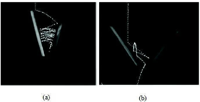
1.2 Experimentally observed particle trajectories for funnels with (a) θ = 60◦ and (b) θ= 40◦. . . 6

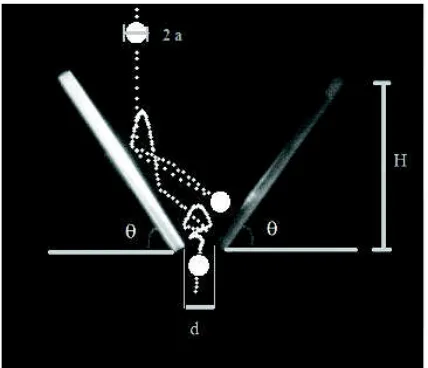
1.3 An image from my experiment showing the system that is used in this thesis for our study of a particle falling through a funnel. H is the height from the bottom of the funnel, ais the radius of the ball, dthe gap at the bottom of the funnel, and θ is the angle of funnel’s walls with the horizontal. . . 8

2.1 Photograph of the experiment used to measure the coefficient of resti-tution. . . 12

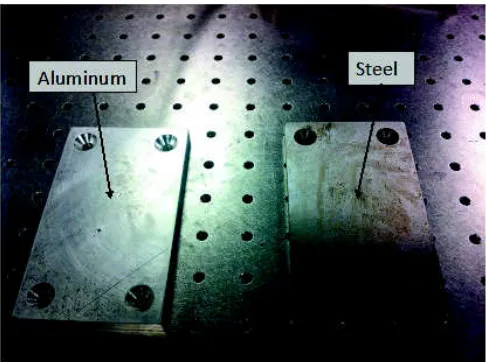
2.2 Schematic of the device used in the coefficient of restitution experiment. 14 2.3 Materials used in restitution coefficient experiment. . . 14

2.4 Photograph of the funnel experiments. . . 16

3.1 Trajectory of an aluminum ball bouncing on the steel plate. . . 19

3.2 Balls used in the restitution coefficient and funnel experiments. . . 20

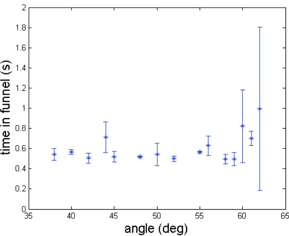
3.3 Time in funnel vs. funnel angle for the ceramic ball and aluminum funnel, restitution coefficient = 0.79±0.10. . . 20

3.4 Simulation results for nondimensionalized time in funnel vs. funnel angle for the ceramic ball and aluminum funnel, restitution coefficient = 0.79±0.10. . . 24

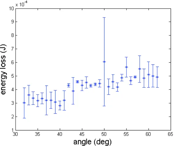
3.5 Energy loss vs. funnel angle for the ceramic ball and aluminum funnel, restitution coefficient = 0.79±0.1 . . . 24

3.6 Time in funnel vs. funnel angle for the Plexiglas ball and steel funnel, restitution coefficient = 0.93±0.01. . . 25

3.7 Simulation results for nondimensionalized time in funnel vs. funnel angle for the Plexiglas ball and steel funnel, restitution coefficient = 0.93±0.01. . . 25

3.8 Energy loss vs. funnel angle for the Plexiglas ball and steel funnel, restitution coefficient = 0.93±0.01. . . 26

3.9 Time in funnel vs. funnel angle for the aluminum ball and steel funnel, restitution coefficient = 0.87±0.05. . . 26

(9)

List of Figures

3.10 Simulation results for nondimensionalized time in funnel vs. funnel angle for the aluminum ball and steel funnel, restitution coefficient = 0.87±0.05. . . 27 3.11 Energy loss vs. funnel angle for the aluminum ball and steel funnel,

restitution coefficient = 0.87±0.05. . . 27 3.12 The trajectory of a ball falling through the funnel measured in six

experiments. (a) Plexiglas ball and steel funnel, e = 0.93±0.01, θ = 60◦. (b) aluminum ball and steel funnel, e = 0.87±0.05, θ = 60◦. (c) ceramic ball and aluminum funnel, e = 0.79±0.1, θ = 60◦. (d) Plexiglas ball and steel funnel, e = 0.93±0.01,θ = 40◦.(e) aluminum ball and steel funnel, e = 0.87±0.05, θ = 40◦.(f) ceramic ball and aluminum funnel, e= 0.790.1, θ = 40◦. . . 28 3.13 Time spent in funnel vs. the initial release location of the ball for the

Plexiglas ball and the steel funnel. (a)θ = 40◦; (b)θ= 50◦; (c) θ= 60◦. 29 3.14 Time spent in funnel vs. the initial release location of the ball for the

aluminum ball and the steel funnel. (a)θ= 40◦; (b)θ = 50◦; (c)θ= 60◦. 30

B.1 Individual high-speed video images Some images by Matlab for bounc-ing aluminum ball on steel flat plate. . . 55 B.2 The trajectory of the bouncing aluminum ball on the steel plate. . . . 55 B.3 Some individual images of the ceramic ball falling through the

alu-minum funnel. . . 56 B.4 The trajectory of the ceramic ball falling through the aluminum funnel

determined by the Matlab program. . . 56

(10)

1

Chapter 1 Introduction

The research reported in this thesis involved studying the dynamics of a single

par-ticle falling through a symmetric funnel under gravity. In this Chapter I introduce

granular materials, review some previous work in areas related to my thesis topic,

and briefly outline my work and the organization of this thesis.

1.1 Granular materials

Granular materials are made up of large numbers of distinct solid particles.

Physi-cists and engineers are interested in understanding the behavior of granular materials

for many reasons. First of all, matter is typically classified as solid, liquid, or gas,

but granular materials are different from all of these and have unique behavior and properties. Sometimes they behave like liquids, as dry sand takes the shape of a

container it is poured into [1]. Although equations that describe the behavior of

tra-ditional solids, liquids and gases are well known, granular materials do not generally

obey these equations and there is no general mathematical description of granular

materials.

Second, granular materials are of great importance and are widely found in our daily life. They were also important in the ancient world and play an important role

in many industries. For example, granular materials are used extensively in farming,

mining, the construction of houses and roads, food products, pharmaceuticals, and

(11)

Chapter 1: Introduction 2

In nearly all applications, contact interactions between particles or between

particles and boundaries are important in determining how the granular materials

behave. Moreover, granular materials often flow through chutes and hoppers but our

understanding of their behavior in these situations is limited [4]. For instance, some

factories use devices to store and transport granular materials that depend on the flow of particles through funnels to direct particles to a desired location, or to control their

speed and flow rate. Understanding the physics of granular flows will help to increase

productivity and maintain the quality and effectiveness of their machines. According

to Ref. [3], many factories that transport and sort granular materials waste 60% of

their power. This is a result of our poor understanding of the behavior of granular

materials. As a result, any improvement in our understanding of how these materials

(12)

1.2 Previous work

In recent years there has been a great deal of interest in the behaviour of granular

flow through funnels and many groups of scientists have obtained significant results

on this and related subjects.

Early work to examine the properties of glass beads flowing in a two dimensional

funnel was done by Le Pennec and co-workers [5] who found a direct link between the flow characteristics and the geometry of the funnel. The behavior of a spherical

particle bouncing inelastically on a vertically vibrating flat surface has been studied

by Mehta and Luck. They found that the particle behaved in a complicated way,

and that the dynamics of the system were difficult to predict [6, 7]. McNamara and

Young discovered that an infinite number of collisions could occur in a finite time in

a system of a finite number of falling particles [8]. Wylie and co-workers studied the

behavior of a one–dimensional system of inelastic particles of different masses flowing through a funnel. They observed that the inelastic particles move in one orbit as a

result of the breakdown a large number of complicated periodic orbits [9, 10]. Gao

and co-workers studied a spherical, inelastic, frictionless particle bouncing in a corner

and found that the particle will either leave the system after making a limited number

of collisions or undergo an unlimited number of collisions in certain time [11].

More recently, there has been a number of studies on the effect of friction on the behavior of granular materials falling through a funnel, such as that by Fang et al. [9],

who showed that the time that the particle spent in the funnel did not decrease

mono-tonically as the angle of the funnel’s walls increased. Spheres in a two-dimensional

vibrating box were modeled by Luding. He found that the behavior of the system

de-pended on the friction of both particles and walls [12]. Brilliantov et al. introduced a

model for collisions in a granular material based on dissipative viscoelastic collisions.

They used the impact velocity to calculate the restitution coefficients for normal and tangential motion. They found there is a direct link between the kind of collision and

(13)

measured the attributes of collisions between small spheres or between small spheres

and a flat plate. Their results showed that a collision model that included friction,

normal restitution, and tangential restitution explained the observed impact behavior

over a large range of incident angles [14].

1.2.1 The work of Wylie and co-workers

Fang et al. [15] performed simulations of a simple system consisting of a single,

inelas-tic, and frictionless particle falling through a symmetric funnel under gravity. They

noted that for certain funnel wall angles, the particle spent more time in the funnel and lost more energy than expected. These phenomena were more pronounced when

the coefficient of restitution of the system was large than when it was small. Figure

1.1 shows the average time spent by the particle in the funnel as a function of the

angle of funnel walls with the horizontal for a restitution coefficient equal to 0.99.

These data where calculated using a simulation code provided to us by Dr. J. Wylie.

While the time spent by the particle in the funnel generally decreases as the angle

increases, there are several peaks in the plot, including a large peak around an angle of 50◦. The simulations of Fang et al. indicated that in these peaks, the particle bounces back and forth between the walls in a simple repeating pattern. This leads

the particle to spend a long time in the funnel. In contrast, away from these peaks

the particle’s trajectory is much more random. Fang et al. also observed that the

sequence of collisions the ball makes with the funnel walls is highly sensitive to the

initial position of the falling ball and to the wall angle. At small angles, the collision

sequence is quite random for all initial positions on the funnel walls, both near to the

centre of the funnel and far from it. At large angles, however, the particle follows a more uniform pattern, especially for initial positions near to the centre of the funnel.

This is illustrated in Figure 1.2, which shows some experimental results that will be

discussed in more detail in Chapter 3. Their theoretical analysis showed that these

phenomena are a result of the existence of neutrally stable quasiperiodic orbits at

(14)

Zhang et al. [4] incorporated friction into these simulations. This is physically

close to the system that we studied experimentally. In their simulations, the system

showed phenomena quite similar to those observed without friction. However, the

frictional system showed the anomalous behaviour at all funnel angles steeper than 45◦ rather than just the small ranges of angles in the frictionless system. Although friction causes the particle to rotate and the dynamics of the particle’s collisions

become more complicated, the particle trajectory at large angles shows a relatively

simple repeating pattern of collisions as in Fig 1.2(a), while at small angles it

(15)

Figure 1.1: Simulation results showing the nondimensionalized average time spent in the funnel as a function of funnel angle for a system with restitution coefficient e= 0.99. Simulations were performed using a Matlab program provided by Prof. J.

Wylie.

(16)

1.3 Outline of this work

For this research, I built a system to study experimentally the behavior of a single

particle falling under gravity through a symmetric funnel as in Figure 1.3. In order

to choose appropriate materials to use for the funnel walls and the ball, I also carried

out an experiment to measure the coefficient of restitution of a variety of different

material combinations. Using funnels made from the chosen materials, I recorded

the trajectory of the balls as they fell through the funnel using a high speed camera. Matlab programs were written to analyze the data obtained from these experiments.

Finally, I compared my results with the theoretical results of Refs. [4, 15]. Our

re-sults are in partial agreement with the theoretical rere-sults of Zhang et al. that were

reported in Ref. [4].

The remaining chapters of the thesis are as follows: In Chapter 2 I describe

the apparatus and the experiments performed. In Chapter 3 I present our results. In addition, I will compare our observations and results with the theoretical results.

(17)

Figure 1.3: An image from my experiment showing the system that is used in this thesis for our study of a particle falling through a funnel. H is the height from the bottom of the funnel, ais the radius of the ball, d the gap at the bottom of the

(18)

9

Chapter 2 Experimental Apparatus and Procedure

As part of the work carried out for this thesis an experimental apparatus for studying

the behavior of a particle falling through a symmetric funnel was designed. In this chapter, we describe our apparatus and discuss the experimental procedures.

2.1 Restitution experiment

An experiment was carried out to measure the restitution coefficient e for various combinations of balls and plates. The restitution coefficient is the ratio of the speed

after a collision to the speed before the collision. Its value is between 0 and 1. e= 0

means the collision is perfectly inelastic ande= 1 means it is perfectly elastic. 1−e2 is the fraction of kinetic energy that remains after a collision between two objects.

The restitution coefficient is an important parameter in our funnel experiments

be-cause the particle loses energy as it falls through the funnel as a result of inelastic

collisions. Ifeis small, the anomalous behavior reported in Ref. [4] is less pronounced, while it is more pronounced for large values.

The apparatus used to measure the restitution coefficient is shown in Figure

2.1; the schematic diagram in Fig 2.2 illustrates the setup of the device. The ball is

dropped from a holder onto a metal plate. The holder has a mechanism to control the

ball’s release. Two plates were used for this experiment, one made from aluminium

and the other from steel. The size of the plates was 12.1 cm x 7.6 cm. The plates are fixed on an optical table by four screws at their corners as seen in Figure 2.3. A high

(19)

Chapter 2: Experimental Apparatus and Procedure 10

the particle as it bounces on the plate. A MiDAS Motion Trigger device is used to

trigger the camera when the ball bounces on the plate. The camera is connected to a

computer which is used to save and analyze the data, and to calculate the restitution

coefficient. Two 500 watt halogen lights are used to illuminate the funnel and the

ball to make them clearly visible in the recorded images.

At the beginning of the experiment, the ball was dropped from a height H

onto the flat plate. The ball is released from the holder with zero initial velocity

and without applying any force other than gravity by moving a small metal tab that

holds the ball in place. The ball bounces several times on the plate before stopping.

The high speed camera records the position of the bouncing ball. The highest height

recorded by the ball after the first collision is h. A matlab program was used to determine h and to calculate the restitution coefficient as follows. The restitution

coefficient is

e= vf

vi

, (2.1)

whereviandvf are the velocity of the ball before and after it hits the plate. Since the

ball is released from rest, its velocity when it hits the plate is given by conservation

of energy as

v_i=p2gH, (2.2)

wheregis the acceleration due to gravity. The ball bounces off the plate with velocity

v_f =evi (2.3)

and rises to a height h. Applying conservation of energy after the collision gives

(20)

so

e= vf

v_i =

r

h

(21)

(22)

2.2 Funnel system

The system used for the funnel experiment reported here consists of a ball holder, the

funnel itself, a high speed camera, and a computer. The ball was released with zero

initial velocity from a height H above the bottom of the funnel and at a horizontal

location x₀ measured from the central axis of the funnel (see Figure 1.3). The

com-ponents of the apparatus are shown in Figure 2.4, which is a photograph of the actual

experimental system. The apparatus mainly consisted of a ball holder which has at its top end a mechanism that controls the ball’s release. The release mechanism was

operated by pulling a thread that moved a metal key, allowing the ball to fall out of

the ball holder. The holder was mounted on a post 40 cm tall. It was also fixed on

a plate that could be moved by adjusting a micrometer screw to adjust the particle’s

starting position. Two different funnels were used for this experiment, one made from

aluminium and the other from steel. The size of the funnel plates was 15.1 cm x 5.3

cm. They are attached by hinges to a pair of horizontal plates as shown in Figure 2.4. The angle of the funnel walls could be adjusted, and was measured with a protractor

with 1.0◦ accuracy. One of funnel walls was fixed on a plate that could be moved by micrometer to adjust the gapdat the bottom of the funnel. The gapdwas measured

using Vernier calipers with 0.02 mm accuracy. A high speed camera was used to

record the position of the particle from the time it enters to the time it leaves the

funnel. The camera is triggered by a MiDAS Motion Trigger when the ball enters the

funnel. The recorded images and the time at which they were taken were sent to the computer for analysis using a Matlab program which is included in Appendix A. The

Matlab program tracked the position of the ball and then calculated its velocity in

each video frame. It then calculated the energy loss at each collision with the funnel

walls, the total energy lost in the funnel, and the time spent in the funnel. Two 500

watt halogen lights illuminate the funnel and the ball to make them clearly visible in

(23)

Figure 2.2: Schematic of the device used in the coefficient of restitution experiment.

(24)

2.3 Data analysis

In order to calculate the total energy that is lost by the sphere, the Matlab code

determined the total energy

E =P +K, (2.6)

E=mgh+ 1

2mv

2_, _(2.7)

where P is the potential energy, K is the kinetic energy, m is the mass of the

par-ticle in kg, g is gravitational acceleration in m.s−2, h is the particle height above the bottom of the funnel, and v is the particle’s velocity in m/s. E, h, v vary with

time while the particle is in the funnel. We calculated the total energy of the ball

when it enters and leaves the funnel using Eq. (2.7) and subtracted these quantities

to get the energy loss. The trajectory of the sphere is determined by the sequence

of collisions it has against the walls, with free-fall motion under gravity between the collisions. We studied the dependence of these quantities on the wall angle θ, e, and

(25)

(26)

17

Chapter 3 Results

3.1 Restitution Coefficient Experiment

The restitution coefficient of several materials was investigated by measuring the

height to which a ball bounced after colliding with plates of different metals. The

restitution coefficient experiment was performed to aid in selecting materials to use

for the funnel experiments. In particular, we wanted to find a system with a high coefficient of restitution in order to make the effects predicted in Ref. [4] more visible.

Figure 3.1 shows an example trajectory followed by an aluminum ball bouncing

on a steel plate. These data are used to calculate the restitution coefficient as outlined

in section 2.2. The results presented here were obtained using ceramic, aluminium

and Plexiglas balls on steel and aluminium plates. Figure 3.2 shows the balls used,

and Table 3.1 gives their mass and radius. Table 3.2 shows the measured values of the

restitution coefficient e for all six ball and plate combinations. These measurements are the average over 30 measurements for each combination and the uncertainties are

found by using the standard deviation of these values. From Table 3.2, we see that the

Plexiglas ball has the highest restitution coefficient with both metal plates. Although

the combination of Plexiglas ball and aluminium plate had a slightly higher

restitu-tion coefficient, we chose to use the combinarestitu-tion of Plexiglas ball and steel plate for

our funnel experiment because we found the phenomena predicted in Ref. [4] were

(27)

Chapter 3: Results 18

3.2 Funnel Experiment

In our experiment, measurements were done on several ball / plate combinations: a

ceramic ball with an aluminum funnel, Plexiglas ball with a steel funnel, and an alu-minum ball with a steel funnel. We studied the time the particle spent in the funnel

and its energy loss as functions of the angle of the funnel walls and the restitution

coefficient of the system.

Figure 3.3 shows the relationship between the angle of the funnel walls and

time the particle spends in the funnel for a ceramic ball bouncing in an aluminum

funnel. For this system, the restitution coefficient is 0.79±0.10. If we ignore the error bars, the average time spent in the funnel initially decreases as the angle of the funnel walls increases. At an angle of approximately 45◦ the time starts to increase again. Experiments were performed for a total of nine different initial positions of

the ball. The holder was positioned at three different positions along the x–axis using

a micrometer screw. At each x–position, the holder was placed at three different

y-positions by using another micrometer screw. The height from which the ball was

released was the same in all cases. The error bars in Figure 3.3 are standard

devia-tions and show how much variation exists in the experimental values. Some of error bars are quite large, suggesting that the time is very sensitive to small uncontrollable

changes of the initial conditions. In order to compare these results with the

theo-retical predictions, we used our values for the restitution coefficient and ball radius

in the simulation software provided to us by Dr. Wylie. The results are shown in

Figure 3.4. At small angles, the average time spent in the funnel decreases as the

angle increases, but the simulation show no increase at higher angles. In this case,

the theoretical and experimental results are similar at small angles but different at large angles. This difference may in part be due to the fact that the simulations were

(28)

Table 3.1: Ball Measurements.

.

Mass Radius

(g) (cm)

Ceramic Ball 4.15±0.10 0.90±0.02 Plexiglas Ball 1.26±0.10 0.70±0.02 Aluminum Ball 3.02±0.10 0.60±0.02

Table 3.2: Restitution Coefficients for different combinations of balls and plates.

.

Ceramic Ball Plexiglas Ball Aluminum Ball Aluminum Plate 0.79±0.10 0.94±0.04 0.85±0.06

Steel Plate 0.79±0.08 0.93±0.01 0.87±0.05

(29)

Figure 3.2: Balls used in the restitution coefficient and funnel experiments.

(30)

Figure 3.5 shows the average energy lost by the ball falling through funnel for

the same materials. The energy lost by the particle in this system is fairly constant at

low funnel angles, but starts to increase around 40◦. This is similar to the theoretical results of Ref. [4]. Again, error bars in Figure 3.5 are the standard deviations. The

error bars reflected the amount of variation in the results at each angle.

Figure 3.6 displays the average time spent in the system for the Plexiglas ball

and steel funnel with e = 0.93±0.01. These data are averaged over a total of nine different initial positions of the ball. The holder was positioned at three different

po-sitions along the x–axis using a micrometer screw. At each x–position, the holder was

placed at three different y–positions by using another micrometer screw. The time is

fairly constant as the funnel angle is varied at small angles, but shows a small peak approximately at 45◦ and an increase starting around 60◦. As before, the large error bars reflect a sensitivity to initial conditions. Figure 3.7 shows the theoretical result

obtained when we use our experimental parameters in Wylie’s simulation program.

At small angles the average time spent in the funnel decreases as the angle increases.

There is a peak between 45◦ and 50◦, then further decrease; there are smaller peaks at higher angles. In this case, the experimental results are quite different from the

theoretical results at small angles. The theoretical results start increasing around 45◦ while our experimental results have an increase starting around 60◦. These difference may again reflect the fact that the simulation was done for a frictionless system while

our experiment was done on a system with friction.

In this case, despite the fact thate was large, we observed much less variation

in the time then in the previous case, for which e was smaller. This contradicts the

theoretical results of Ref. [4] which predicted that the anomalous behavior should be more pronounced for a higher restitution coefficient.

Figure 3.8 shows the energy lost by the Plexiglas ball falling through the steel

funnel. The data at each angle are averaged over nine different initial positions of

(31)

behavior is seen in the theoretical results for a similar restitution coefficient in Ref. [4]

The results for the aluminum ball and the steel funnel, with restitution

coeffi-cient e= 0.87±0.05, are shown in Figures 3.9–3.11. As displayed in Figure 3.9, the average duration of the aluminum ball during the steel funnel is fairly constant with increasing angle of the funnel walls, but shows a sharp increase around 59◦. In order to compare this result with the theoretical result, we use our values of the restitution

coefficient and ball radius in Wylie’s simulation software. The results in Figure 3.10

show that the average time spent in the funnel decreases as the angle increase with a

small peak around an angle of 50◦. In this case, theoretical and experimental results are different. Again, these differences may be because the simulation were done for a

frictionless system while the experiments did have friction.

Figure 3.11 displays the average energy loss of the aluminum ball in the steel

funnel. The energy loss increases as the angle increases. This combination, which

consists of an aluminum ball and steel funnel, and the previous combination, which

consists of a Plexiglas ball and steel funnel, have similar experimental results for time

spent in the funnel and energy lost as a function of funnel walls angle. Although

these two systems have higher restitution coefficients than the ceramic ball and alu-minum funnel, we found they showed less pronounced anomalous behavior than the

system with the smallest restitution coefficient. This disagrees with the theoretical

predictions of Refs. [4, 15].

Figure 3.12 illustrates the experimentally observed trajectories of the balls as

they fall through the funnels. One observes that at large angles for all three systems

the balls bounce back and forth across the funnel many times in a regular pattern. On the other hand, at small angles, the balls bounce much more randomly through

the funnels. The former case leads to an increase in the time spent in the funnel, and

because the number of collisions increases, to a corresponding increase in the energy

(32)

Figure 3.13 and Figure 3.14 show the results of experiments performed to show

how the time spent in funnel depended on the starting locationsx₀ of the ball, where

x₀ is measured from the centre of the funnel. Figure 3.13 shows results for the

Plex-iglas ball and the steel funnel at angles 40◦, 50◦, and 60◦, and Figure 3.14 shows results for the aluminum ball and the steel funnel at similar angles. These figures illustrate how much the duration is sensitive to the starting location. Figure 3.13(a)

and Figure 3.14(a) show that in both systems the duration at an angle of 40◦ is quite scattered, indicating a very high sensitivity to initial location. At this angle, the ball’s

trajectory in quite random, as seen in Fig 3.12(d) and (e). On the other hand, Figure

3.13(c) and Figure 3.14(c) show that at high angles the duration varies smoothly with

initial position. At this angle, the ball’s trajectories follow a more organized pattern

(33)

Figure 3.4: Simulation results for nondimensionalized time in funnel vs. funnel angle for the ceramic ball and aluminum funnel, restitution coefficient = 0.79±0.10.

(34)

Figure 3.6: Time in funnel vs. funnel angle for the Plexiglas ball and steel funnel, restitution coefficient = 0.93±0.01.

(35)

Figure 3.8: Energy loss vs. funnel angle for the Plexiglas ball and steel funnel, restitution coefficient = 0.93±0.01.

(36)

Figure 3.10: Simulation results for nondimensionalized time in funnel vs. funnel angle for the aluminum ball and steel funnel, restitution coefficient = 0.87±0.05.

(37)

Figure 3.12: The trajectory of a ball falling through the funnel measured in six experiments. (a) Plexiglas ball and steel funnel, e= 0.93±0.01, θ= 60◦. (b) aluminum ball and steel funnel,e= 0.87±0.05, θ= 60◦. (c) ceramic ball and

aluminum funnel, e= 0.79±0.1, θ= 60◦. (d) Plexiglas ball and steel funnel, e= 0.93±0.01,θ= 40◦.(e) aluminum ball and steel funnel,e= 0.87±0.05,

(38)

(a)

(b)

(c)

(39)

(a)

(b)

(c)

(40)

31

Chapter 4 Discussion and Conclusion

4.1 Discussion

The results presented in Chapter 3 will now be discussed and compared with the

theoretical work of Refs. [4, 15]

Some of our experimental results agree well with the theoretical prediction for

a frictionless particle that falls under gravity and bounces through a 2-dimensional

funnel. On the other hand, however, we also found several differences between them.

Theoretically, for a system with e = 1, peaks in the plot of the time spent in the

funnel vs. angle are seen at certain angles at which neutrally stable periodic orbits

were shown to exist. For e < 1, the peaks observed are caused by the existence of

quasi-periodic orbits. Theoretically, peaks are found with simple orbits. For a simple orbit, the locations of the collisions tend to be relatively far from the funnel exit

which makes the particle bounce back and forth in a quasi-periodic orbit for a long

time as the particle moves down towards the exit of the funnel. However, for more

complicated orbits, the locations of the collisions are led to be relatively close to the

funnel exit which allows the particle to leave the funnel after only a short time in

the funnel. When e is small, the particle loses more energy at each collision, and so

leaves the funnel quickly even in simple orbits at highθ. Because of this, the anoma-lous behavior will become less pronounced as the value of the restitution coefficient

decreases [4, 15]. In contrast, our experimental results shown in Figures 3.3, 3.6, and

3.9 show the opposite behavior. The experimental funnel system with the smallest

(41)

Chapter 4: Discussion and Conclusion 32

with the larger restitution coefficients. This is a surprising result.

The simulation results show peaks in the time spent in the funnel around

fun-nel angles of 45◦, 60◦ because at these angles, the particle bounces back and forth many times in a coherent sequence of collisions before leaving the funnel. Comparing that with our results we also observed changes around 45◦. While we do not see a peak like that in the simulation, we do see a change in the character of the

trajec-tories, as shown in Figure 3.12, that is similar to that seen in the simulations. For

angles less than 45◦, the particles in our experiments bounced in a complicated and non-repeating pattern, while at angles greater than 45◦, they bounced in a coherent repeating pattern.

The simulation results showed that the time spent in funnel by a frictionless

particle decreases slightly as the angle of the funnel walls increases, and at angles

steeper than 45◦, the decrease continues but with small peaks around some angles. Our results also showed a decrease of the time spent in the funnel as the angle

in-crease. The reasons for that differences would be because the simulations were done

for a frictionless particle while in reality friction exists between any two contacting

surfaces and will have an effect even it is small. Ref. [4] pointed out that friction causes the ball to rotate, leading to a more complicated trajectory, but these

com-plicated orbits become more simple at high angles. Moreover, when the effects of

friction are included, the predicted behavior appeared at all angles steeper than 45◦ rather than around certain angles as for the frictionless particle. Another possible

factor that is the degree of smoothness of the funnel surfaces may contribute to the

differences between experiment and theory. Surface roughness or small craters in the

surface produced by earlier impacts could affect the results. Finally, variations in humidity and temperature of the laboratory where the experiments were performed

could also change the condition of the funnel walls.

Both the theoretical and our experimental results showed that, at small angles,

(42)

position of particle, while at higher angles, the time is much less sensitive to initial

position. At low angles, the particle bounced between the left and right funnel walls

on complicated and non-repeating trajectories, while at large angles, the particle

(43)

4.2 Conclusion

The goal of our study was to experimentally investigate behaviour of a single spherical

particle falling through a symmetric funnel. From high-speed video recording of the

trajectory of the sphere, we were able to measure the time that the particle spends

in the funnel, and the energy it loses as a function of the angle of the funnel walls for

different restitution coefficients. This behaviour was simulated by Wylie et al. and

explained theoretically by them. By comparing our results with the theoretical work, we observed that some of our results were similar to those reported in Refs. [4, 15]

while other results were not, and we interpreted our results in terms of the theoretical

predictions.

Theoretically, the anomalous behavior is predicted to be more pronounced for

higher values of the coefficient of restitution. Surprisingly, in our experimental work

these effects are more pronounced for lower values of the coefficient of restitution. Compared with the theoretical work, our experiment shows some phenomena similar

to those reported in Refs. [4, 15]. In particular, the increase in time spent in the

funnel observed above 45◦ for the ceramic ball in the aluminum funnel is consistent with the simulations discussed in Refs. [4, 15]. It is likely that this behaviour is due

to the fact that the particles bounce back and forth across the funnel many times at

steep angles, as seen in Figure 3.11 and in agreement with the theoretical work.

The time spent in the funnel for particles in all systems are highly sensitive to

the starting position of the falling particle on the funnel walls. At steep angles of the

funnel walls, the trajectory of the particle is more regular than that for small angles,

where it is quite random. The trajectories of the falling particle at angles steeper

(44)

4.3 Future work

Our experimental results provide support and confirmation for some of the simulation

results for the behavior of a single particle falling through a symmetric funnel under

gravity. On the other hand, some of our results disagree with the theoretical results.

There is a number of questions related to our results that could be addressed in future

work.

-We found the results to change when the surface condition of the ball or funnel

walls changed. It would be useful to study and understand the behavior of a particle

in a symmetric funnel for different controlled surface conditions. .

-It would be useful to investigate several different ball and funnel materials with

different restitution coefficients using the same technique that we used.

-We found some of our results agree with the theoretical work while others

disagree. These effects are complex and cannot be fully understood from our

ex-periment. It would be interesting to investigate these phenomena further by using

a larger funnel in a fully computer-controlled experiment, in which the computer is

(45)

36

References

[1] Ming Gao, Jonathan J. Wylie and Qiang Zhang, American Institute of

Mathe-matical Sciences, 8(1), 275293 (2009).

[2] Troy Shinbrot and Fernando J. Muzzio, Phys. Today, 53(3), 25 (2000).

[3] Heinrich M. Jaeger, Sidney R. Nagel, and Behringer. “The

Physics of Granular Materials”. Physics Today, 32 (1996)

http://jfi.uchicago.edu/granular/introduction.html.

[4] Qiang Zhang, Yuan Fang, and Jonathan J. Wylie, Phys. Rev. E 83, 051303 (2011).

[5] T. Le Pennec, M. Ammi, J. C. Messager, and A. Valance, Eur. Phys. J. B 7, 657

(1999).

[6] A. Mehta and J. M. Luck, Phys. Rev. Lett. 65, 393 (1990).

[7] J. M. Luck and A. Mehta, Phys. Rev. E 48, 3988 (1993).

[8] S. McNamara and W. R. Young, Phys. Fluids A 4, 496 (1992).

[9] J. J. Wylie and Q. Zhang, Phys. Rev. E 74, 011305 (2006).

[10] R. Yang and J. J. Wylie, Phys. Rev. E 82, 011302 (2010).

[11] M. Gao, J. J.Wylie, and Q. Zhang, Commun. Pure Appl. Anal. 8, 275(2009).

[12] S. Luding, Phys. Rev. E 52, 4442 (1995).

[13] N. V. Brilliantov, F. Spahn, J. M. Hertzsch, and T. Poschel, Phys. Rev. E 53,

5382 (1996).

[14] S. F. Foerster, M. Y. Louge, H. Chang, and Kh. Allia, Phys. Fluids 6, 1108

(46)

Appendix : Discussion and Conclusion 37

[15] Yuan Fang, Ming Gao, Jonathan J. Wylie, and Qiang Zhang, Phys. Rev. E 77,

(47)

38

Appendix A

The Matlab Code

A.1: The Matlab code used to calculate the time spent in the funnel and the energy loss for the particle

c l e a r a l l ,

c l c

c c=hsv( 3 ) ; % c o l o r scheme

d e g r e e l i s t=F o l d L i s t ; % e x t r a c t t h e l i s t o f d e g r e e f o l d e r s

a n g l e s=d e g r e e l i s t ( : , 1 : 2 ) ; % e x t r a c t t h e a n g l e s ( u s u a l l y , 20 t o 62)

%f p r i n t f ( ’%d d e g r e e f o l d e r s found\n ’ , s i z e ( d e g r e e l i s t , 1 ) ) ;

% i n i t i a l i z e t h e m a t r i x t o s t o r e t h e a v e r a g e d v a l u e s

a v e r a g e t i m e s=zeros(s i z e( d e g r e e l i s t , 1 ) , 3 ) ;

e r r o r t i m e s=zeros(s i z e( d e g r e e l i s t , 1 ) , 3 ) ;

a v e r a g e h i t s=zeros(s i z e( d e g r e e l i s t , 1 ) , 3 ) ;

e r r o r h i t s=zeros(s i z e( d e g r e e l i s t , 1 ) , 3 ) ;

a v e r a g e e n e r g i e s=zeros(s i z e( d e g r e e l i s t , 1 ) , 3 ) ;

e r r o r e n e r g i e s=zeros(s i z e( d e g r e e l i s t , 1 ) , 3 ) ;

f i g u r e( 3 )

f o r degree num =1:s i z e( d e g r e e l i s t , 1 )

d e g r e e f o l d e r=d e g r e e l i s t ( degree num , : ) ;

cd( d e g r e e f o l d e r ) ;

disp( [ ’ c u r r e n t f o l d e r : ’ d e g r e e f o l d e r ’ , c u r r e n t a n g l e : ’ ,

a n g l e s ( degree num , : ) ] ) ;

p o s i t l i s t =F o l d L i s t ; % e x t r a c t t h e l i s t o f p o s i t i o n f o l d e r s

(48)

Appendix A: The Matlab Code 39

( u s u a l l y , 1 t o 3 )

%f p r i n t f ( ’%d p o s i t i o n f o l d e r s found\n ’ , s i z e ( p o s i t l i s t , 1 ) ) ;

subplot(c e i l(sqrt(s i z e( d e g r e e l i s t , 1 ) ) ) ,

c e i l(sqrt(s i z e( d e g r e e l i s t , 1 ) ) ) , degree num ) ;

hold on ;

f o r posit num =1:s i z e( p o s i t l i s t , 1 )

p o s i t i o n f o l d e r= p o s i t l i s t ( posit num , : ) ;

cd( p o s i t i o n f o l d e r ) ;

disp( [ ’ c u r r e n t f o l d e r : ’ d e g r e e f o l d e r ’\’ p o s i t i o n f o l d e r ’ ,

c u r r e n t p o s i t i o n : ’ , p o s i t i o n s ( posit num , : ) ] ) ;

e x p e r i m e n t l i s t=F o l d L i s t ; % e x t r a c t t h e l i s t o f e x p e r i m e n t f o l d e r s

e x p e r i m e n t s=e x p e r i m e n t l i s t ( : , 2 :end) ; % e x t r a c t t h e e x p e r i m e n t

numbers ( u s u a l l y , 1 t o 1 0 )

%f p r i n t f ( ’%d e x p e r i m e n t f o l d e r s found\n ’ , s i z e ( e x p e r i m e n t l i s t , 1 ) ) ;

% i n i t i a l i z e t h e v e c t o r s used f o r a v e r a g i n g

T o t a l t i m e i n f u n n e l=zeros(s i z e( e x p e r i m e n t l i s t , 1 ) , 1 ) ;

T o t a l n u m b e r o f h i t s=zeros(s i z e( e x p e r i m e n t l i s t , 1 ) , 1 ) ;

T o t a l e n e r g y l o s t=zeros(s i z e( e x p e r i m e n t l i s t , 1 ) , 1 ) ;

f o r exp num =1:s i z e( e x p e r i m e n t l i s t , 1 )

e x p e r i m e n t f o l d e r=e x p e r i m e n t l i s t ( exp num , : ) ;

cd( e x p e r i m e n t f o l d e r ) ;

disp( [ ’ c u r r e n t f o l d e r : ’ d e g r e e f o l d e r ’\’ p o s i t i o n f o l d e r

’\’ e x p e r i m e n t f o l d e r ’ , c u r r e n t e x p e r i m e n t :

’ , e x p e r i m e n t s ( exp num , : ) ] ) ;

b m p F i l e s = d i r( ’∗. bmp ’ ) ;

[ T o t a l t i m e i n f u n n e l ( exp num ) , T o t a l n u m b e r o f h i t s ( exp num ) ,

T o t a l e n e r g y l o s t ( exp num ) ] = RunExp ( b m p F i l e s ) ;

cd . . ; % go b a c k t o e x p e r i m e n t f o l d e r s

end

plot( T o t a l t i m e i n f u n n e l , ’ c o l o r ’ , c c ( posit num , : ) , ’ LineWidth ’ , 2 ) ;

legend( s t r c a t ( ’ p o s i t i o n ’ ,num2str( p o s i t i o n s ) ) ) ;

x l ab el( ’ e x p e r i m e n t #’ ) ;

(49)

%c a l c u l a t e t h e c u r r e n t s e t d a t a

a v e r a g e t i m e s ( degree num , posit num )=sum( T o t a l t i m e i n f u n n e l )

/s i z e( T o t a l t i m e i n f u n n e l , 1 ) ;

e r r o r t i m e s ( degree num , posit num )=std( T o t a l t i m e i n f u n n e l ) ;

a v e r a g e h i t s ( degree num , posit num )=sum( T o t a l n u m b e r o f h i t s )

/s i z e( T o t a l n u m b e r o f h i t s , 1 ) ;

e r r o r h i t s ( degree num , posit num )=std( T o t a l n u m b e r o f h i t s ) ;

a v e r a g e e n e r g i e s ( degree num , posit num )=sum( T o t a l e n e r g y l o s t )

/s i z e( T o t a l e n e r g y l o s t , 1 ) ;

e r r o r e n e r g i e s ( degree num , posit num )=std( T o t a l e n e r g y l o s t ) ;

%f p r i n t f ( ’%d e x p e r i m e n t ( s ) :\n a v e r a g e time i n f u n n e l : %d\n a v e r a g e

number o f h i t s : %d\n a v e r a g e e n e r g y l o s t : %d\n ’ , exp num ,

a v e r a g e t i m e s ( degree num , posit num ) , a v e r a g e h i t s

( degree num , posit num ) , a v e r a g e e n e r g i e s ( degree num , posit num ) ) ;

cd . . ; % go b a c k t o p o s i t i o n f o l d e r s

end

hold o f f ;

cd . . ; % go b a c k t o d e g r e e f o l d e r s

end

a n g l e s=str2num( a n g l e s ) ; % c o n v e r t b e f o r e p l o t t i n g

f i g u r e( 4 )

hold on ;

f o r plot num =1:s i z e( a v e r a g e t i m e s , 2 )

%p l o t ( a n g l e s , a v e r a g e t i m e s ( : , p l o t n u m ) , ’ c o l o r ’ , cc ( plot num , : ) ) ;

errorbar( a n g l e s , a v e r a g e t i m e s ( : , plot num ) , e r r o r t i m e s ( : , plot num ) ,

’ c o l o r ’ , c c ( plot num , : ) , ’ LineWidth ’ , 2 ) ;

end

hold o f f ;

t i t l e( ’ Average t i m e s i n a f u n n e l ’ ) ;

(50)

y l ab el( ’ a v e r a g e time , s ’ ) ;

legend( ’ p o s i t i o n 1 ’ , ’ p o s i t i o n 2 ’ , ’ p o s i t i o n 3 ’ , ’ p o s i t i o n 4 ’ , ’ p o s i t i o n 5 ’ ) ;

f i g u r e( 5 )

hold on ;

f o r plot num =1:s i z e( a v e r a g e h i t s , 2 )

errorbar( a n g l e s , a v e r a g e h i t s ( : , plot num ) , e r r o r h i t s ( : , plot num ) ,

end

hold o f f ;

t i t l e( ’ Average h i t s ’ ) ;

x l ab el( ’ a n g l e , deg ’ ) ;

y l ab el( ’ a v e r a g e h i t s ’ ) ;

f i g u r e( 6 )

hold on ;

f o r plot num =1:s i z e( a v e r a g e e n e r g i e s , 2 )

errorbar( a n g l e s , a v e r a g e e n e r g i e s ( : , plot num ) , e r r o r e n e r g i e s ( : , plot num ) ,

end

hold o f f ;

t i t l e( ’ Average e n e r g y l o s t ’ ) ;

x l ab el( ’ a n g l e , deg ’ ) ;

y l ab el( ’ a v e r a g e energy , J ’ ) ;

%p o s i t i o n s =[1 , 2 , 3 , 4 , 5 ] ; % change t o f i t t h e e x a c t l o c a t i o n s

%f i g u r e ( 7 )

% t i t l e ( ’ Average t i m e s i n a f u n n e l ’ ) ;

%f o r p l o t n u m =1: s i z e ( a v e r a g e t i m e s , 1)

%s u b p l o t ( c e i l ( s q r t ( s i z e ( a v e r a g e t i m e s , 1 ) ) ) ,

(51)

plot( p o s i t i o n s , a v e r a g e t i m e s ( plot num , : ) ,

% l e g e n d ( s t r c a t ( num2str ( a n g l e s ( p l o t n u m ) ) , ’ d e g r e e ’ ) ) ;

% x l a b e l ( ’ i n i t i a l l o c a t i o n , m’ ) ;

% y l a b e l ( ’ a v e r a g e time , s ’ ) ;

%end

f p r i n t f( ’ Done !\n ’ ) ;

\2 n d s e t{l a n g u a g e=Matlab , numbers= l e f t , c a p t i o n=The Program f o r c a l c u l a t e

t h e a v e r a g e t i m e s s p e n t and t h e a v e r a g e e n e r g i e s l o s s , c a p t i o n p o s=b}

\renewcommand\l s t l i s t i n g n a m e{Program}

function [ T o t a l t i m e i n f u n n e l , T o t a l n u m b e r o f h i t s , T o t a l e n e r g y l o s t ]

= RunExp ( b m p F i l e s )

T o t a l t i m e i n f u n n e l =0;

T o t a l n u m b e r o f h i t s =0;

T o t a l e n e r g y l o s t =0;

i f isempty( b m p F i l e s ) % no . bmp f i l e s i n t h e f o l d e r

f p r i n t f( 2 , ’No . bmp f i l e s i n t h i s f o l d e r !\n ’ ) ;

return

end

j =0;

d o t p o s i t i o n i = [ ] ;

d o t p o s i t i o n j = [ ] ;

f i l e n a m e = b m p F i l e s (round(length( b m p F i l e s ) / 2 ) ) . name ;%p i c k t h e m i d d l e s h o t

I c o l o r = imread ( f i l e n a m e ) ; %I c o l o r i s t h e m i d d l e s h o t

f i l e n a m e = b m p F i l e s ( 1 ) . name ; %p i c k t h e f i r s t s h o t

I 0 = imread ( f i l e n a m e ) ; %I 0 i s t h e f i r s t s h o t

I c o l o r m a p = I c o l o r − I 0 ; %d i f f e r e n c e image

(52)

s e n s i t i v i t y = 0 . 2 5 ;

gauge = dot max − dot max∗s e n s i t i v i t y ;

s e n s i t i v i t y f u n n e l = 0 . 7 ;

g a u g e f u n n e l = dot max − dot max∗s e n s i t i v i t y f u n n e l ;

s e n s i t i v i t y b a l l = 0 . 2 5 ;

g a u g e b a l l = dot max − dot max∗s e n s i t i v i t y b a l l ; %s e t t h e b r i g h t n e s s which

i s c o n s i d e r e d t o be a b a l l

f o r t 1 =1:(s i z e( Icolormap , 1 ) )

f o r t 2 =1:(s i z e( Icolormap , 2 ) )

d i f f = dot max − I c o l o r m a p ( t1 , t 2 ) ;

i f d i f f == 0

row pos = t 1 ; %r o w p o s i s t h e y−c o o r d i n a t e o f t h e b r i g h t e s t s p o t

c o l p o s = t 2 ; %c o l p o s i s t h e x−c o o r d i n a t e o f t h e b r i g h t e s t s p o t

end

i n d e x b a l l = f i n d( ( I c o l o r m a p ( row pos , : ) )>g a u g e b a l l ) ; %” t h e b a l l ” p o i n t s

a l o n g t h e row pos

r a d i u s b a l l = i n d e x b a l l (s i z e( i n d e x b a l l , 2 ) ) − i n d e x b a l l ( 1 ) ; %t h e w i d t h

o f t h e b a l l

m a s s b a l l = 0 . 0 0 3 0 1 9 ; %Kg

g = 1 0 ; %m/ s ˆ2

% p o s i t i o n o f t h e f u n n e l ==================================================

kk =0;

f o r i n d 0 1 =1:s i z e( I0 , 1 )

kk=kk +1;

I 0 L = [ ] ;

I0 R = [ ] ;

(53)

I 0 R c o l = [ ] ;

I 0 L c o l e n d ( kk ) = 0 ;

I 0 R c o l e n d ( kk ) = 0 ;

I 0 r o w e n d ( kk ) = i n d 0 1 ;

% L e f t h a l f o f t h e f u n n e l ===========

f o r i n d 0 2 = 1 : ( (round(s i z e( I0 , 2 ) ) ) / 2 + 1 )

i f ( I 0 ( ind01 , i n d 0 2 ))>g a u g e f u n n e l

I 0 L =[ I 0 L I 0 ( ind01 , i n d 0 2 ) ] ;

I 0 L c o l = [ I 0 L c o l i n d 0 2 ] ;

I 0 L c o l e n d ( kk ) = I 0 L c o l (s i z e( I 0 L c o l , 2 ) ) ;

end

% R i g h t h a l f o f t h e f u n n e l ============================

f o r i n d 0 3 =((round(s i z e( I0 , 2 ) ) ) / 2 + 2 ) : 1 : (round(s i z e( I0 , 2 ) ) )

i f ( I 0 ( ind01 , i n d 0 3 ))>g a u g e f u n n e l

I0 R =[ I0 R I 0 ( ind01 , i n d 0 3 ) ] ;

I 0 R c o l = [ I 0 R c o l i n d 0 3 ] ;

I 0 R c o l e n d ( kk ) = I 0 R c o l (s i z e( I 0 R c o l , 1 ) ) ;

end

[ f u n n e l c o l i n d e x t o p l e f t , f u n n e l r o w i n d e x t o p l e f t ] = f i n d

( I 0 L c o l e n d ˜=0 , 1 , ’ f i r s t ’ ) ;

[ f u n n e l c o l i n d e x b o t t o m l e f t , f u n n e l r o w i n d e x b o t t o m l e f t ]

= max( I 0 L c o l e n d ) ;

i n d e x = f i n d( I 0 R c o l e n d ˜=0);

(54)

f u n n e l c o l i n d e x t o p r i g h t = I 0 R c o l e n d ( i n d e x ( 1 ) ) ;

[ f u n n e l c o l i n d e x b o t t o m r i g h t , I I ] = min( I 0 R c o l e n d ( i n d e x ) ) ;

f u n n e l r o w i n d e x b o t t o m r i g h t = i n d e x ( I I ) ;

I 0 r o w = s i z e( I0 , 1 ) : (−1 ) : 1 ;

% p o i n t s d e s c r i b i n g t h e f u n n e l −−−−−−−−−−−−−−−−−−−−−−−−−−−−−−−−−−−−−−−−−−−−

y0 L = s i z e( I0 , 1 ) − f u n n e l r o w i n d e x b o t t o m l e f t ;

x0 L = f u n n e l c o l i n d e x b o t t o m l e f t ;

y1 L = s i z e( I0 , 1 ) − f u n n e l r o w i n d e x t o p l e f t ;

x1 L = f u n n e l c o l i n d e x t o p l e f t ;

y0 R = s i z e( I0 , 1 ) − f u n n e l r o w i n d e x b o t t o m r i g h t ;

x0 R = f u n n e l c o l i n d e x b o t t o m r i g h t ;

y1 R = s i z e( I0 , 1 ) − f u n n e l r o w i n d e x t o p r i g h t ;

x1 R = f u n n e l c o l i n d e x t o p r i g h t ;

t e t a L = atan( (abs( y1 L−y0 L ) ) / (abs( x1 L−x0 L ) ) ) ;

t e t a R = atan( (abs( y1 R−y0 R ) ) / (abs( x1 R−x0 R ) ) ) ;

%==========================================================================

s t a r t f r a m e n u m = [ ] ;

end frame num = [ ] ;

%================

c o l l i s i o n L w i n g = 0 ;

c o l l i s i o n R w i n g = 0 ;

%−−−−−−−−−−−−−−−−−−−

f o r k = 2 :length( b m p F i l e s )

f i l e n a m e = b m p F i l e s ( k ) . name ; %s t a r t from t h e second image

I 1 = imread ( f i l e n a m e ) ;

(55)

and t h e f i r s t one

max order = [ ] ;

f o r i n d =1:s i z e( I , 2 )

[m( i n d ) , i n d e x r o w ( i n d )]=max( I ( : , i n d ) ) ; %m( i n d ) s t o r e s t h e

max v a l u e i n t h e ” i n d ” column , i n d e x r o w ( i n d ) s t o r e s i t s row i n d e x

max order =[ max order m( i n d ) ] ; %max order s t o r e s

t h e max v a l u e s o f each column

end

[ maxim , i n d e x c o l ]=max( max order ) ; %maxim s t o r e s t h e

max v a l u e o f t h e whole image, i n d e x c o l s t o r e s i t s column i n d e x ;

%t h a t ’ s where t h e p e a k s s t a r t t o i n t e r c h a n g e

c a u s i n g t h e f a l s e d e t e c t i o n

%s e t u p an i n d e x c o l as a MIDDLE POINT o f t h e b a l l , not t h e BRIGHTEST ONE

t h e b a l l = f i n d( ( max order)>g a u g e b a l l ) ;

i f ˜isempty( t h e b a l l ) % i f t h e b a l l i s s t i l l somewhere i n t h e p i c t u r e

i n d e x c o l=round( ( t h e b a l l (1)+ t h e b a l l (end) ) / 2 ) ;

end

d o t p o s i ( k ) = i n d e x r o w ( i n d e x c o l ) ;

d o t p o s j ( k ) = i n d e x c o l ;

maximum( k ) = maxim ;

i f maxim > gauge %i f t h e maximum v a l u e ”maxim” i s w i t h i n t h e b a l l

( t h e b r i g h t n e s s i s o v e r 1 5 5 ,

%t h e i n d e x c o l s t a n d s f o r i t s column i n t h e image

%t h e i n d e x r o w s t a n d s f o r i t s row i n t h e image

% time f o r t h e b a l l t o be i n t h e f u n n e l ===============================

i f (s i z e( I ,1)−d o t p o s i ( k))>f u n n e l r o w i n d e x t o p l e f t

s t a r t f r a m e n u m = [ s t a r t f r a m e n u m k ] ;

end

(56)

end frame num = [ end frame num k ] ;

end

%======================================================================

j = j +1;

d o t p o s i t i o n i = [ d o t p o s i t i o n i s i z e( I ,1)−d o t p o s i ( k ) ] ;

d o t p o s i t i o n j = [ d o t p o s i t i o n j d o t p o s j ( k ) ] ;

%−−−−−−−−−−−−−−−−−−−−−−−−−−−−−−−−−−−−−−−−−−−−−−

end

%−−−−−−−−−−−−−−−−−−−−−−

I 0 f l i p u d = f l i p u d( I 0 ) ;

%f i g u r e ( 1 )

%p l o t ( d o t p o s i t i o n j , d o t p o s i t i o n i , ’ o−’)

% t i t l e ( ’ P a r t i c l e T r a j e c t o r y i n a Funnel ’ )

%f i g u r e ( 2 )

%imshow ( I 0 f l i p u d )

%h o l d on ;

%p l o t ( d o t p o s i t i o n j , d o t p o s i t i o n i , ’ w . ’ )

% f o r pp = 1 : l e n g t h ( d o t p o s i t i o n j )

% t e x t ( d o t p o s i t i o n j ( pp ) , d o t p o s i t i o n i ( pp ) , s p r i n t f ( ’(% d,%d ) ’ ,

d o t p o s i t i o n j ( pp ) , d o t p o s i t i o n i ( pp ) ) , ’ C o l o r ’ , [ . 6 . 8 . 6 ] )

% end

%s e t ( gca , ’ y d i r ’ , ’ normal ’ )

%a x i s ( [ 0 480 0 4 2 0 ] )

%a x i s ( [ 0 s i z e ( I , 2 ) 0 s i z e ( I , 1 ) ] )

%h o l d o f f ;

%−−−−−−−−−−−−

NFperS = 2 5 0 ;

n u m o f f r a m e s = end frame num ( 1 ) − s t a r t f r a m e n u m ( 1 ) ;

T o t a l t i m e i n f u n n e l = n u m o f f r a m e s∗( 1 / NFperS )∗1 0 ;

%d i s p ( [ ’ T o t a l time i n t h e f u n n e l : ’ num2str ( T o t a l t i m e i n f u n n e l ) ’ [ s e c ] ’ ] )

(57)

Hit L = 0 ; %r e s e t t h e c o u n t e r f o r l e f t−s i d e h i t s

Hit R = 0 ; %r e s e t t h e c o u n t e r f o r r i g h t−s i d e h i t s

W= [ ] ; %s t o r e t h e e n e r g i e s o f each h i t

c o l l i s i o n p o s i t i o n c o l L = [ ] ; %d e c l a r e t h e v e c t o r s t o r i n g columns o f t h e

l e f t−s i d e h i t e l e m e n t s

c o l l i s i o n p o s i t i o n r o w L = [ ] ; %d e c l a r e t h e v e c t o r s t o r i n g rows o f t h e

l e f t−s i d e h i t e l e m e n t s

c o l l i s i o n p o s i t i o n c o l R = [ ] ; %d e c l a r e t h e v e c t o r s t o r i n g columns o f

t h e r i g h t−s i d e h i t e l e m e n t s

c o l l i s i o n p o s i t i o n r o w R = [ ] ; %d e c l a r e t h e v e c t o r s t o r i n g rows o f

t h e r i g h t−s i d e h i t e l e m e n t s

E n e r g y d i f f e r e n c e L = [ ] ; %d e c l a r e t h e l e f t−s i d e e n e r g y d i f f e r e n c e v e c t o r

E n e r g y d i f f e r e n c e R = [ ] ; %d e c l a r e t h e r i g h t−s i d e e n e r g y d i f f e r e n c e v e c t o r

V in R = [ ] ; %d e c l a r e t h e r i g h t−s i d e incoming v e l o c i t i e s v e c t o r

V out R = [ ] ; %d e c l a r e t h e r i g h t−s i d e outcoming v e l o c i t i e s v e c t o r

V in L = [ ] ; %d e c l a r e t h e l e f t−s i d e incoming v e l o c i t i e s v e c t o r

V out L = [ ] ; %d e c l a r e t h e l e f t−s i d e outcoming v e l o c i t i e s v e c t o r

%d o t p o s i t i o n i − v e c t o r o f t h e b a l l ’ s v e r t i c a l c o o r d i n a t e s

%d o t p o s i t i o n j − v e c t o r o f t h e b a l l ’ s h o r i z o n t a l c o o r d i n a t e s

%d i f − v e c t o r o f t h e b a l l ’ s h o r i z o n t a l v e l o c i t i e s

f o r i i =1:(s i z e( d o t p o s i t i o n i ,2)−1)

d i f = [ d i f d o t p o s i t i o n j ( i i +1)−d o t p o s i t i o n j ( i i ) ] ;

end

%f i g u r e ( 3 )

%p l o t ( d i f )

% t i t l e ( ’ P a r t i c l e V e l o c i t y d i r e c t i o n i n a Funnel ’ )

t h r e s h = 1 . 5 ;%d e f i n e t h e t h r e s h o l d f o r t h e change

which i s c o n s i d e r e d a h i t

VERT = 1 ; %s t a r t w i t h v e r t i c a l movement

(58)

% 0 − moving v e r t i c a l l y ,

% +1 − moving t o t h e r i g h t .

d i f =[ d i f d i f (s i z e( d i f , 2 ) ) ] ; % i n c r e a s e t h e l e n g t h o f t h e d i f v e c t o r

f o r j j =2:s i z e( d i f , 2 ) %scan e v e r y l o c a t i o n

i f (abs( d i f ( j j ))<t h r e s h && VERT==1) % s l o w or no s p e e d b e f o r e

t h e f i r s t h i t

MOV( j j )=0; %t h e b a l l moves v e r t i c a l l y

end

i f ( (abs( d i f ( j j ))>= t h r e s h && d i f ( j j ) <0) | | (abs( d i f ( j j ))<t h r e s h

&& VERT==0 && d i f ( j j ) <0)) && ˜ (VERT==0 && d i f ( j j ) <0 && d i f ( j j −1)>=0

&& d i f ( j j +1) >=0) | | (VERT==0 && d i f ( j j ) >=0 && d i f ( j j −1)<0 && d i f ( j j +1) <0)

% s m a l l n e g a t i v e s p e e d a f t e r t h e f i r s t h i t or f a s t n e g a t i v e s p e e d

( e x c l u d i n g t h e one−time d i p s ) :

MOV( j j )=−1; %t h e b a l l moves t o t h e l e f t

VERT=0; %f i r s t h i t has o c c u r e d

end

i f ( (abs( d i f ( j j ))>= t h r e s h && d i f ( j j ) >=0) | | (abs( d i f ( j j ))<t h r e s h

&& VERT==0 && d i f ( j j ) >=0)) && ˜ (VERT==0 && d i f ( j j ) >=0 && d i f ( j j −1)<0

&& d i f ( j j +1) <0) | | (VERT==0 && d i f ( j j ) <0 && d i f ( j j −1)>=0 && d i f ( j j +1) >=0)

% s m a l l p o s i t i v e s p e e d a f t e r t h e f i r s t h i t or f a s t p o s i t i v e s p e e d

( e x c l u d i n g t h e one−time d i p s ) :

%f p r i n t f ( ’ At %d t h e b a l l moves t o t h e r i g h t : %d .\n ’ , j j , d i f ( j j ) ) ;

MOV( j j )=1; %t h e b a l l moves t o t h e r i g h t

VERT=0; %f i r s t h i t has o c c u r e d

end

%p r o c e s s t h e MOV so t h a t t h e r e ’ s no d i p s :

f o r mm=2:(s i z e(MOV,2)−1)

i f MOV(mm−1)<0 && MOV(mm) >=0 && MOV(mm+1) <0 %one−s h o t

l e f t w a l l h i t

(59)

end

i f MOV(mm−1)>=0 && MOV(mm) <0 && MOV(mm+1) >=0 %one−s h o t

r i g h t w a l l h i t

MOV(mm)=1;

end

f o r j j =2:s i z e( d i f , 2 )

i f MOV( j j )<MOV( j j−1) % 0−>(−1) or 1−>(−1) − r i g h t w a l l h i t

Hit R = Hit R +1;

c o l l i s i o n p o s i t i o n r o w R = [ c o l l i s i o n p o s i t i o n r o w R

d o t p o s i t i o n i ( j j ) ] ; %ok

c o l l i s i o n p o s i t i o n c o l R = [ c o l l i s i o n p o s i t i o n c o l R

d o t p o s i t i o n j ( j j ) ] ; %ok

d i n = sqrt( ( d o t p o s i t i o n j ( j j ) − d o t p o s i t i o n j ( j j −1))ˆ2

+ ( d o t p o s i t i o n i ( j j ) − d o t p o s i t i o n i ( j j −1 ) ) ˆ 2 ) ; %ok

d o u t= sqrt( ( d o t p o s i t i o n j ( j j ) − d o t p o s i t i o n j ( j j +1))ˆ2

+ ( d o t p o s i t i o n i ( j j ) − d o t p o s i t i o n i ( j j + 1 ) ) ˆ 2 ) ; %ok

v i n = d i n ;

v o u t = d o u t ;

%f p r i n t f ( ’ P o t e n t i a l : %d −−> %d\n ’ , m a s s b a l l∗g

∗d o t p o s i t i o n i ( j j −1) , m a s s b a l l∗g∗d o t p o s i t i o n i ( j j ) ) ;

%f p r i n t f ( ’ K i n e t i c : %d −−> %d\n ’ , ( 0 . 5 )∗m a s s b a l l∗( v i n ˆ 2 ) ,

( 0 . 5 )∗m a s s b a l l∗( v o u t ˆ 2 ) ) ;

E n e r g y i n = m a s s b a l l∗g∗d o t p o s i t i o n i ( j j−1)

+ ( 0 . 5 )∗m a s s b a l l∗( v i n ˆ 2 ) ;

E ne rgy out= m a s s b a l l∗g∗d o t p o s i t i o n i ( j j )

+ ( 0 . 5 )∗m a s s b a l l∗( v o u t ˆ 2 ) ;

W = [W ( E n e r gy i n−E ne rgy out ) ] ;

%E n e r g y d i f f e r e n c e R=sum (C)/ l e n g t h (C ) ;

The Behavior of a Falling Particle in a Funnel

Scholarship@Western

Scholarship@Western

The Behavior of a Falling Particle in a Funnel

The Behavior of a Falling Particle in a Funnel

The Behavior of a Falling Particle in a

Funnel

Certificate of Examination

Abstract

Acknowledgements

Table of Contents

List of Tables

List of Figures

Chapter 1

Introduction

1.1

Granular materials

1.2

Previous work

1.2.1

The work of Wylie and co-workers

1.3

Outline of this work

Chapter 2

Experimental Apparatus and Procedure

2.1

Restitution experiment

2.2

Funnel system

2.3

Data analysis

Chapter 3

Results

3.1

Restitution Coefficient Experiment

3.2

Funnel Experiment

Chapter 4

Discussion and Conclusion

4.1

Discussion

4.2

Conclusion

4.3

Future work

References

Appendix A

The Matlab Code