Article
Experimental Study and Modeling of Ground-Source
Heat Pumps with Combi-Storage in Buildings
Wessam El-Baz*1 ID, Peter Tzscheutschler1ID and Ulrich Wagner1
1 Institute of Energy Economy and Application Technology, Technical University of Munich. Arcisstr. 21 80333 Munich, Germany
* Correspondence: [email protected]; Tel.: +49-(0)89-289-28314
Abstract:There is a continuous growth of heat pump installations in residential buildings in Germany. The heat pumps are not only used for space heating and domestic hot water consumption but also to offer flexibility to the grid. The high coefficient of performance and the low cost of heat storages made the heat pumps one of the optimal candidates for the power to heat applications. Thus, several questions are raised about the optimal integration and control of the heat pump system with buffer storages to maximize its operation efficiency and minimize the operation costs. In this paper, an experimental investigation is performed to study the performance of a ground source heat pump (GSHP) with a combi-storage under several configurations and control factors. The experiments were performed on an innovative modular testbed that is capable of emulating a ground source to provide the heat pump with different temperature levels at different times of the day. Moreover, it can emulate the different building loads such as the space heating load and the domestic hot water consumption in real-time. The data gathered from the testbed and different experimental studies were used to develop a simulation model based on Modelica that can accurately simulate the dynamics of a GSHP in a building. The model was validated based on different metrics. Energetically, the difference between the developed model and the measured values was only 3% and 4% for the heat generation and electricity consumption, respectively.
Keywords:Modelica; testbed; control requirements; modeling; EMS; sensor placement;
0. Introduction
In the German power sector, an ongoing increase of renewable energy integration can be witnessed. In 2016, 29% of gross generated electricity was produced from renewable energy sources’ (RES’s), which represents 192 TWh [1]. Such increase in the RES’s integration is empowered by several policies such as the renewable energy act (EEG) [2]. The act guarantees the generator a fixed price over a specific term, which gives a priority to the RES in the electricity market. Having such weather dependent fluctuating RES in the market, raised the demand for flexibility to balance the fluctuating generation. Sector coupling presented one way to mitigate the fluctuating RES and offer flexibility to the grid. Hence, it is receiving continuous attention not only within the research communities but also on the political and industrial level. Coupling the power to the heat sector is seen as one of the most influential and attractive approaches to decarbonize the heat sector and gain additional flexibility in power gird [3]. Considering that the consumed heat energy in Germany within different sectors was 1,373 TWh in 2016 [4], there is a substantial room for power to heat application integration. An advantage of such applications is its attractive costs due to its dependency on heat storage that has significantly lower costs compared to batteries.
The heat pump is a major role player in sector coupling due to the progressive improvement of the coefficient of performance (COP) [5]. Hence, the number of heat pumps installations are on
continuous growth on yearly basis, especially in the residential sector. According to [6], the heat pump installations in new buildings in 2016 reached 31.8%. Heat pump represents 34% of the market share of the single-family houses, 16% of the multi-family houses and 13.6% of the non-residential buildings. Such widespread of the heat pump raised research questions focusing not only on the heat pump cycle and components improvement but also on a better integration and control of the heat pump as a system.
The topics discussed within the literature covered large scope such as the thermodynamic cycle and compressor optimizations [7–10] hydraulic system configurations [11], performance evaluation [12,13], and integration in district heating and smart grids [5,14]. The research presented can be divided into experimental studies and numerical studies. The experimental studies were mostly oriented towards cycle and components optimization of the heat pumps. In [15], a carbon dioxide direct-expansion heat pump was investigated in different operating conditions. [16] studied the performance of solar ground source heat pump in dual heat source coupling modes to optimize the average system COP. Furthermore, [17] experimentally tested a gas engine driven heat pump for different operation modes. The author developed a prototype to test the heating and cooling performance for different evaporator’s inlet temperatures, ambient temperatures, and gas engine speeds. The numerical studies and simulations were utilized, where experimental studies would be costly. In [18], a heat pump was simulated to cover the load of a multi-zone office building. While in [19], a simulation model was developed to analyze the flow pumping of ground source heat pumps. [20] developed a numerical model for a reversible multi-function heat pump to evaluate its performance in summer for domestic hot water (DHW) and space cooling. The numerical model was then evaluated against a model in TRNSYS.
In the residential sector, several studies were performed on air-source heat pumps (ASHP) and ground-source heat pumps (GSHP). The presented studies were mostly numerical. Also, it is oriented towards optimizing the heat pump control, system dimension and hydraulics to minimize the operation costs and maximize the use of renewable energies within the residential building as in [21–25]. Although numerical studies can provide relatively proper indicator of the behavior of a system, it is exposed to several uncertainties and its accuracy is always questioned, especially if the studied object is a thermodynamic system. Studies analyzing large models on the district level or micro grid levels have mostly 1-h resolution as in the review of [3], consequently, all dynamics of the heat pump systems are concealed. Moreover, in several cases, the COP is assumed to be constant and all the nonlinearities are ignored so that the optimization problem can converge faster. Yet, this exposes the model to inevitable uncertainties. On the building level, dynamic systems simulation programs are used such as TRNSYS or Modelica-based software as Simulation X [26]. These programs can detail the dynamics of the systems, yet as discussed in [27], calibration is rather complicated. Moreover, these models are mostly validated by a plausibility check, but not against measured values. Field tests were performed to investigate the performance of heat pumps [12]. These studies can provide a realistic investigation of the performance of heat pumps in general, yet it does not offer the flexibility of an experimental system to vary different parameter and it can conceal several details that can contribute to the understanding of the system.
0.1. Objectives
• Presenting a novel modular heat pump testbed design that emulates a complete residential house. It includes a ground-source emulator, combi-buffer heat storage, and a building load emulator. The testbed is designed to be integrated with different heat pump types and hydraulic connections, so that it can be used for standardization applications, control and optimization methods performance testing, and models validation
• Based on multiple experimental testing, the real-life optimal control criteria for a commercial residential GSHP under the given constraints of the heat pumps manufactures have been identified.
• Demonstrating a modelica-based heat pump model that can be easily integrated into building and district simulations due to its minimal computational requirements. The model was also validated and calibrated based on the experimental data of the presented testbed.
The structure of this paper is as follows: Section1describes the design and components of the testbed. Moreover, it introduces the measurements system used and discusses the testbed control dynamics. Section2presents the experimental testing procedure and its purpose. Section3presents the validated Modelica heat pump model and its structure. Section4discusses the results of the experimental testing and the validation of the Modelica model. Section5presents a conclusive summary of the experimental study and the model performance.
1. Experimental System Description
1.1. Overview
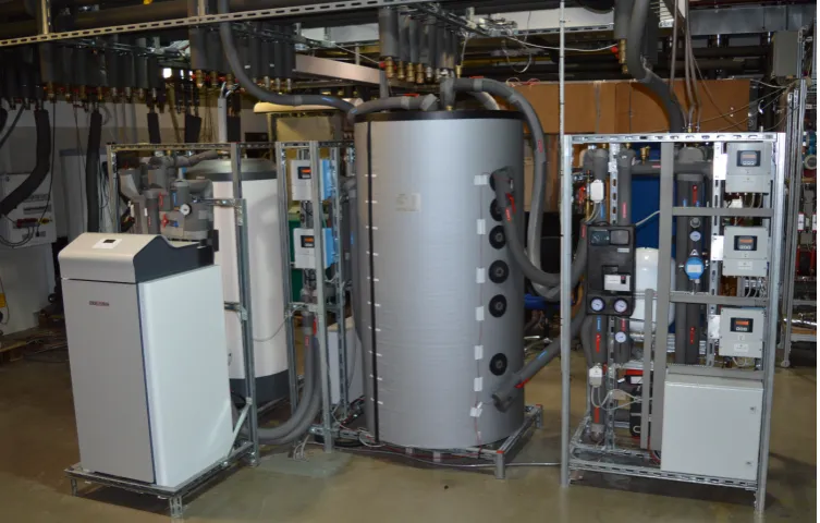
The testbed consists of 3 different modules: ground-source emulator (A), combi-storage (B), and the building loads emulator (C). Figure1and2show a simplified hydraulic scheme and the real testbed, respectively. The presented hydraulic configuration is not a permanent configuration, but rather the one used for the experiments documented in this paper. Other possible configuration can be also implemented such as a direct connection between the heat pump and module C, replacing module B with a DHW tank module, or having two separate modules for a DHW tank and a buffer tank. Each module has its own independent control and measurement system to facilitate the integration of different modules. The GSHP used is a STIEBEL ELTRON WPF10 heat pump with a thermal power of 10.31 kW and a COP of 5.02 by B0/W35 according to the standard EN 14511. A brine pump and heating system circulation pump is already integrated within the GSHP. Moreover, the GSHP is also equipped with an emergency/backup electrical heater of 8.8 kW.
Figure 2.The 3 modules and the heat pump installation in the lab
1.2. Module A: ground-source emulator
Module A emulates a ground-source, which is equivalent to a controlled environment room for the ASHP. The module consists of a 300-liter storage that is heated by a 12.5 kW electrical heater. This storage is filled with a water-glycol mixture as an anti-freezing heat transfer fluid. The electrical heater is controlled via a hysteresis regulator to maintain a maximum set-temperature for the whole tank of 40◦C. The hysteresis limits can be adjusted based on the user settings. To deliver a specific temperature profile to the heat pump, a conventional SH mixer is used to mix the supply of the storage with the return of the heat pump till it reaches the required temperature. This types of mixers can lead to a slow reaction towards changes in the set points but provides a rather stable output as discussed later in section1.6.
1.3. Module B: Combi-storage module
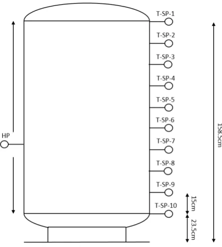
This module represents one of the storage system configurations in a residential household. The storage system consists of a 749 l combi-hygienic buffer storage for SH and DHW consumption. The cold water is heated via a stainless steel heat exchanger that goes through the length of the tank to supply DHW. Furthermore, a coaxial pipe is inserted in this heat exchanger to enable DHW circulation and maintain a proper hot water temperature in the pipes.
Figure 3.Sensors position across the combi-storage
1.4. Module C: Building loads emulator
This module is the most complicated as it has to represent the SH of a household and DHW consumption. The SH circuit consists of a mixer, as in figure1, that mixes the hot water supply of the tank with the return of the SH circuit to reach the required set temperature. The building heating load is then made present via using heat exchangers that are cooled via a cooling system. The flow rate of the cooling system is the one influencing the building load magnitude and defining the return temperature of the SH circuit. Such flow rate is controlled via a motor control valve that positions the valve according to the required set point. Within the SH circuit, two heat exchangers are available of different powers and capacities. One heat exchanger is dedicated to old building heating loads that can reach up 20 kW and have a high flow rate, while the other one is only for new buildings with a maximum power of 7 kW. Two motor valves are used to switch between the two heat exchanger as per the testbed setup.
The hot water consumption is realized via three magnetic valves representing three different types of taps within the household. These valves can present different activities such as showering, washing, and cooking. The flow rate of the valves can be adjusted manually to match the standard flow rate of the activity. To show the effect of the hot water consumption on the heat storage and heat pump, a household profile of the hot water consumption can be delivered to the testbed so that the opening and closing time and duration of the water tapping can be defined for the different valves. Consequently, a similar energetic profile can be executed.
The DHW circulation pump is managing the circulation exactly as in a conventional household circulation pump. The pump can be switched on or off based on a circulation schedule or hot water temperature in the pipe. The circulated load is presented via a heat exchanger that is cooled via the fresh water supply, similar to the SH circuit heat exchanger. Such design was adopted for different testbeds in the labs of the institute for energy economy and application technology (IfE) as shown in [29].
1.5. Measurement system
Hence, for a temperatureTof 65◦C, the tolerance is±0.28◦C. To maximize the accuracy further, a temperature sensor calibration device of a higher accuracy was used.
Magnetic inductive flow measurements devices are used to measure the volume flow rate. The flow measurements devices were already calibrated by the manufacturer, consequently no additional calibration was performed. For the nominal flow rate, the error of the devices varied between 0.2% and 0.5% depending on the sensor type and the size of the pipe.
The electrical power of the heat pump is measured via a 3-phase electricity meter (KDK PRO 380) of class B accuracy, which is 1% according to the EN 50470-1/3. The meter is connected to the measurement system via MODBUS RTU connection, that communicates the power, currents, and voltages of the 3 phases each second.
The sensors and actuators of the whole testbed are connected to National instruments (NI) compact reconfigurable IO (cRIO) chassis and modules that receive and send different digital or analog inputs and outputs. The control program and data logger are based on LabVIEW that runs on a conventional PC.
1.6. System and control dynamics
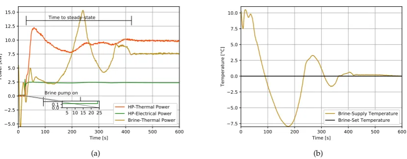
The main purpose of the testbed is to show the detailed dynamics of a heat pump system to be able to develop and validate a realistic numerical model. In figure4(a), the start dynamics of the heat pump can be shown. As soon as the heat pump starts, the brine pump operates for 24 seconds, then the compressor is switched on. It takes the testbed 393 seconds to reach the steady state due to the mixer control dynamics, yet it does not influence significantly the thermal power of the heat pump. The brine power fluctuating from 2.5 till 15.1 kW led only to fluctuations of 10±2.5 kWth, within those 393
seconds. The mixer controller effect can be more clearly described in figure4(b). For a set temperature of 0◦C, the mixer started to mix the tank temperature with the return of the heat pump. Due to both of the start dynamics of the mixer supply and heat pump return, the fluctuations occurred within the time to steady state. Yet, once a steady state is reached the mixer controller can maintain the set temperature, while minimizing the fluctuations.
0 100 200 300 400 500 600
Time [ ] −5.0 −2.5 0.0 2.5 5.0 7.5 10.0 12.5 15.0 Power [kW]
Brine pump on Time to teady-state
HP-Thermal Power HP-Electrical Power Brine-Thermal Power 5 10 15 20 25
0.0 0.1
(a)
0 100 200 300 400 500 600
Time [s] −7.5 −5.0 −2.5 0.0 2.5 5.0 7.5 10.0 Temperature [°C] Brine-Supply Temperature Brine-Set Temperature (b)
Figure 4.Starting dynamics of the heat pump testbed, (a)Thermal and electrical power of the heat pump, in addition to the thermal power of the Brine circuit (b) Brine supply temperature dynamics because of the mixer circuit
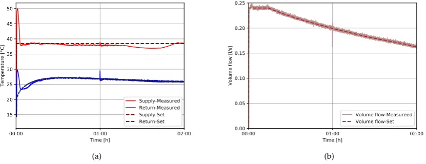
the tolerance reaches±3 K. A smaller tolerance was required to accurately emulate a building load profile on the testbed. The return temperature was more accurately controlled as the motor valve has a continuous PID controller. Consequently, a tolerance of±0.1 to±0.15 K was achieved, which is challenging considering the low inertia of the system (i.e. the water volume of the system is small compared to a real building).
The volume of the flow rate of the heating system circulation pump was also controller via a PID controller. In figure5(b), the measured set and measured flow rate are presented. It can be deduced that the pump and the controller were able to flow accurately the set temperature with a tolerance less than 0.01 l/s. The graph was plotted against the same time of measurements of the supply and return temperature, to be able to show the dynamics of the two graphs simultaneously.
00:00 01:00 02:00
Time [h] 15
20 25 30 35 40 45 50
Temperature [°C]
Supply-Measured Return-Measured Supply-Set Return-Set
(a)
00:00 01:00 02:00
Time [h] 0.00
0.05 0.10 0.15 0.20 0.25
Volume flow [l/s]
Volume flow-Measureed Volume flow-Set
(b)
Figure 5.Control dynamics of module C, (a) supply and return temperature of the space heating circuit (b) flow rate of the space heating circuit
2. Experimental Testing Procedure
Four major experiments are covered within the scope of this paper, as in figure6. The first group of experiments is to define the performance map of the heat pump. This group of experiments analyzes the given heat pump performance under different heating supply temperature and brine temperatures. On the system scale, the second group of experiments investigates the optimal SH and DHW sensor position and reveals its effect on the overall system performance in buildings. In the third and fourth group of experiments, the optimal control rules for EMS are defined through testing the cycling effect. In a residential heat pump, the control parameters are limited to a boolean signal to switch the heat pump on or off. Consequently, an EMS in a residential building does not have any influence on other technical parameters such as the flow rate of brine pump or the controller of the heating circuit between the heat pump and the combi-storage. Based on these constrains, the heat pump optimal control rules can be defined. In cycling effect experiment with constant continuous load, the thermal load is given to the building emulator (e.g. 5 kW), constant through the whole 24 hours, while heat pump had to cycle between on and off. Within this group of experiments, 4 experiments were performed with a duty cycle of 50%. The switching time was varied between 1, 2, 3, and 4 h. 6 h duration was not performed in this experiment due to the limited thermal capacity of the combi-storage. To maintain the energy balance, the thermal loadQSHwas limited to 50% of the nominal thermal power of the heat
pumpQN. Cycling effect was also tested while trying to maintain a constant return temperature. The
QSHwas limited to 80% ofQN. Due to the increase ofQSH, the 6-h cycle was made possible. Thus, 6
Through this set of experiments, the characteristic of the operation of the heat pump can be clarified, in addition to the impact of sensor installation position. Moreover, the results of the cycling effect experiments can provide a clear picture about the optimal control criteria of GSHP.
Figure 6.Flow of the experimental procedures
3. Modelica Based Model
According to [30], the heat pump modeling approaches into physical, black box and grey box approach. The physical approach can forecast the dynamic behavior of a system. Hence, it is often used for heat pump design and parameters optimization. Black boxes can be easily computed and are useful for large systems, yet it is usually concealing several system dynamics to maintain its simplicity. Grey box models try to achieve a balance between the two aforementioned approaches. For residential buildings modeling, three main criteria have to be satisfied:
• simplicity: the model has to be easily computable as the building modeling software such as the Modelica and TRNSYS are not yet powerful enough to solve the equations of multiple complicated dynamic systems simultaneously
• accuracy: the model has to minimize the uncertainties of the results
• dynamic: the model should not be concealing the dynamic behavior of the heat pump under different operating conditions.
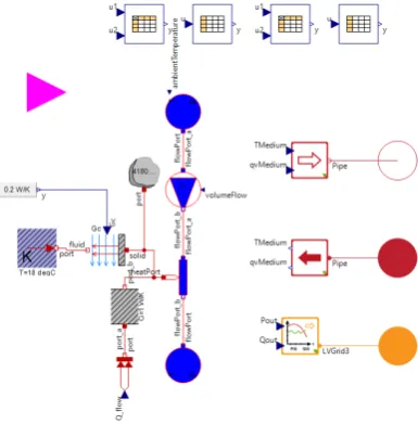
In this paper, a semi-empirical dynamic model is presented that was developed on Modelica. Figure7shows a view of the structure of the model in Modelica. It was designed such that it can be coupled with Open Modelica Library [31] or Simulation X "Green City" Package [32]. Consequently, the basic model components were designed based on the Open Modelica Library, yet a separable interface was included to connect to the "Green City" package. The simulated thermal power of the heat pumpQsimand the coefficient of performanceCOPsimare calculated empirically based on the
collected experiments performed in section2. TheQsimis calculated then as a function of the brine
based on those two inputs either directly from the experimental tabulated data or from the empirical equation given in2. This polynomial equation was formulated based on data fitting algorithm of the experimental data. TheR2is 0.99, while the sum squared error and the root mean squared error is 0.1727 and 0.0759, respectively. The electrical power of the heat pumpPsimis then simply calculated
based on equation3.
Qsim= f(Tb,Ts) (1)
COPsim= f(Tb,Ts)
=11.16+0.2488×Tb−0.2282×Ts−0.003031×TbTs+0.001405×Ts2
(2)
Psim =
Qsim
COPsim
(3)
Although the powers and COP of the heat pump can be accurately calculated using the presented equation, these data will not be sufficient to present the system dynamics such system thermal losses, system inertial, operation time of the brine pump before the compressor starts, resting time between two consecutive starts, and time to full power. Consequently, the calculated full power from the equation1is given as a prescribed thermal power to a thermal pipe directly. This pipe represents the outlet pipe of the heat exchanger of the condenser. Between the pipe and the prescribed heat model, there is a thermal resistor that was empirically calibrated to present conduction losses. The inertia of the system is represented by a thermal capacitor that can be initialized based on the system water volume as in equation4,whereCpis the specific heat capacity of water,Volis the internal water
volume of the heat pump,ρis the density of water. The convection losses was modeled as shown in figure7, assuming that the room temperature is always fixed at a value of 18◦C. The convection heat loss factor was also empirically estimated and set as fixed value throughout the whole simulation.
C=Cp×Vol×ρ (4)
Through the presented model, the aforementioned criteria for heat pump modeling for building simulations can be satisfied without adding any additional complexity to the heat pump model. Adding any additional details such as modeling the thermodynamic cycle would not contribute to the quality of the results in this situation as these variables are not monitored within the study of the dynamic behavior of a building.
4. Results
4.1. Experimental Analysis
4.1.1. System Performance
As explained in section2, the initial phase of the experimental study is to analyze the performance map of the given heat pump. Figure8shows the behavior of the COP as a function of the supply temperature and the brine temperature. At each of the measured points ofTbandTs, the set points
were held constant and measurement was taken as an average of 40 minutes of operation to maintain a proper steady and accurate measurements. The set points are defined as a discrete set of integers such thatTs ∈ {35, 40, 45, 50, 55, 60, 65}andTb ∈ {−5, 0, 10, 15, 20}. In figure8, the measurements at 65◦C
was eliminated, as the heat pump can not operate atTb =−5 andTs=65 simultaneously. As shown,
the COP increases as the supply temperature decrease and the brine temperature increases. The range of the COP is quite wide between 1.6 and 8.0. This means that the costs of operation of the heat pump to generate 1 kWh of heat can reach up to 500% compared to the cost of the most optimal possible operation. Consequently, it is a must to supply the numerical models with an accurate measured data, otherwise building model can be exposed to high uncertainties.
−5 0 5 10 15
Brine temperature [°C] 35
40 45 50 55 60
Supply temperature [°C]
1.6 2.4 3.2 4.0 4.8 5.6 6.4 7.2 8.0 COP
Figure 8.Performance map of the integrated GSHP
4.1.2. Sensors Position
System setup and configuration in the building has also a significant influence on the behavior of the COP of the heat pump. In the field study of [12], the impact of an efficient planning and installation on the heat pump seasonal performance factor was investigated. The installation process does not only include hydraulic system but also the DWH and SH sensors positioning on the storage system. Although direct connection of the SH circuit to the buildings without any buffer storage can lead to the most optimal operation, buffer storages are necessary to offer flexibility as in [33]. In the literature, different research discussed the sensor position. In [11], different sensors positions along a combi-storage were tested based on a simulation model. It was found that as the DHW sensors distances from the SH zone, the lower is the number of starts per year. In [26,34], it was stated that the DHW sensor has no influence on the performance of the heat pump, yet the higher the position the better. Moreover, the author stated that sensors at a lower position can help in decreasing the set temperature while maintaining comfort.
calculated according to equation5, whereEthandEelis the accumulated thermal and electrical energy
within a defined period, respectively.
COPAverage=
Eth
Eel
(5)
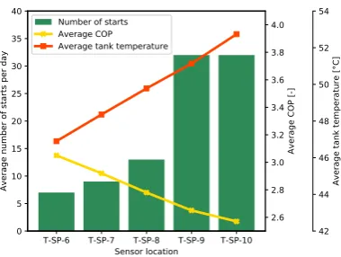
The sensor positions on the x-axis can be clarified through figure3. For each sensor position, the measurement was repeated for 3 consecutive days, then the average of the 3 days was taken. At T-SP-10 and T-SP-9 which are the lowest two sensors, the value of the number of starts is similar and significantly higher than the rest of positions. This means that if a sensor has to be allocated at a lower position on the tank as per the theoretical studies, this zone (below T-SP-9) has to be ignored for sensors allocations. As the sensor is positioned more towards the upper zone of the tank, the lower is the number of starts per day. This means also that the storage heat content decreases because the useful volume that is kept at the set temperature decreases as indicated in equation6[35], whereAsis
area of the storage,Tsetis the required set temperature andTstorage(h)is the temperature across the
length of the storageh.
Estorage =ρ×Cp×As×
Z h
0
(Tstorage(h)−Tset)dh
∀Tstorage(h)>Tset
(6)
On the other hands, as the average tank temperature decreases, the average COP also linearly increases, which fits the behavior presented by the performance map in8. Between T-SP-10 and T-SP-6, the average COP increased by 21.5%, which is a significant increase that influences the economics of the heat pump considering that no intelligent control algorithms were yet deployed. The direct correlation between the average COP and the average tank temperature shows that COP is solely dependent on the tank set temperature.
T-SP-6 T-SP-7 T-SP-8 T-SP-9 T-SP-10 Sensor location 0 5 10 15 20 25 30 35 40
Average number of starts per day
7 9
13 3232
2.6 2.8 3.0 3.2 3.4 3.6 3.8 4.0
Average COP [-]
Number of starts Average COP Average tank temperature
42 44 46 48 50 52 54
Average tank temperature [°C]
Figure 9.Sensor location influence on the number of starts, average COP, and average tank temperature
4.1.3. Cycling Influence on the System Performance
In the first experiment as explained in section2, a constant continuous load is set for SH circuit, which is almost equal to 50% of the nominal heating power of the heat pump. Hence, the space heating load was set toQSH =5.0 kW. Figure10(a)showsEth,Eel,Ebrineand the average COP for 1-h on/off
cycle till 4-h on/off cycle, whereEbrineis thermal energy extracted from the brine circuit. 1-h on/off
the electricity consumed is the lowest. The heat generated is almost constant. It has varied only between 113.85 kWh to 115.2.
Although 1-h cycle has the highest number of starts, it achieved the highest COP because it maintained the lowest possible tank temperature. Having the heat pump operating for 4 hours then stopping for 4 hours while having a constant demand from the SH circuit means that the heat pump has to heat the buffer storage to higher temperatures to satisfy the demand during the off (i.e. resting time). Although the 4-h cycle minimized the number of starts to only 3 times per day, it does not lead to an optimal efficient operation. The average COP was lowered by 13%. The lower number of starts might increase the lifetime of the compressor, yet this is not a measurable factor that can be assessed easily by a testbed or even within a field study at the moment. If it would be included, a cost of start has to be evaluated to reach an optimal control schedule.
In the second experiment, the QSH was increased to 8 kW and the QSH was not set to be
continuous, but cycling similar to the heat pump. The reason behind increasing the power of the load and the simultaneous cycling is to consume immediately the delivered power of the heat pump and to maintain the lowest possible return temperatureTr. In this case, 1-h to 6-h cycles were used as the
heat storage was almost not used. Through this experiment, it can be noticed that the average COP is almost constant and was not influenced by either the long or short duration of heat pump operation. The energiesEth,Eel, andEbrinevaried only by 2.7%, 1.5% and 1.136 %, respectively. Such variation
is partially due to the measurement errors and the minor difference in the initial conditions of the experiment.
To summarize the output of these experiments, it can be deduced that if a buffer or combi-storage are combined with the heat pump:
• The long operation duration to minimize the heat pump number of starts reduces the average COP and consequently can lead to a lower seasonal performance factor (SPF)
• If the heat pump is delivering directly while minimally using the heat storage or without a heat storage, the long duration of operation has no impact on the average COP of the system
113 114 115 116
E_th [kWh]
28 30 32 34
E_el [kWh]
86 88 90
E_brine [kWh]
1-h 2-h 3-h 4-h
ON/OFF cycle duration 3.4
3.6 3.8 4.0
Average COP [-]
(a)
112 114 116
E_th [kWh]
30.5 31.0 31.5 32.0
E_el [kWh]
86 87 88 89
E_brine [kWh]
1-h 2-h 3-h 4-h 6-h
ON/OFF cycle duration 3.60
3.65 3.70
Average COP [-]
(b)
4.2. Model Validation
To validate the model, the heat pump described in section3was integrated with a SimulationX heat storage and building model described in [32]. The red box in figure11shows the heat pump on the right side and the controller. The storage is presented by the storage icon, which is connected to the heat pump on one side and a mixer on the other side. On the far right side comes the building model and the weather data. The most important parameters of the storage are indicated in table1. The default parameters have been used for the rest of the components. The heat pump controller has two different hysteresis models that control both ofTsandTstorage. Hence, the heat pump can only
be switched on when both of the controllers generate a true signal. Different building models can be integrated from [32], yet a generic model was set to model a cycling load similar to the one presented in the previous section so that the dynamics of both the thermal and electrical power, in addition to the supply and return temperatures can be visualized and validated.
Figure 11.Modelica heat pump model integrated with the building storage model of Simulation X
Table 1.Heat storage parameters
Description Value Units[-]
Heat storage Volume 749 l
Diameter of heat storage 0.79 m
Heat Conductance of isolation 2 WK
Number of heat storage layers 10
-Ambient temperature 18 ◦C
Maximum layer temperature 65 ◦C
Heat transmission coefficient for neighboring layers 465 mW2.K
measurement is only 3.08% and 4.18% for heat generation and electricity consumption, respectively. These minor variations indicate that the presented model can accurately simulate the heat pump and deliver proper results once it’s integrated into a building model.
00:00 06:00 12:00 18:00 23:59 Time [h]
0 2 4 6 8 10 12 14 16
Power [kW]
HP-Thermal Power HP-Electrical Power Sim-Thermal Power Sim-Electrical Power
(a)
00:00 06:00 12:00 18:00 23:59 Time [h]
20 25 30 35 40
Temperature [°C]
HP Supply HP Return Sim-HP Supply Sim-HP Return
(b)
Figure 12.Temperatures and power dynamics of both the simulation model and the measurements of the testbed, (a) thermal and electrical power (b) supply and return temperatures
Heat Generation Electricity Consumption 0
20 40 60 80 100 120
Energy [kWh]
Measurement Simulation
Figure 13. Comparison between the measurements and the simulation model based on the heat generation and the electricity consumption
The computational speed of the model was also tested on Simulation X. A backward differentiation formula (BDF) solver was used to compute the model on a personal computer having the minimum calculation step size, maximum calculation step size, absolute tolerance, relative tolerance, minimum step size, and recording of the results equal to 1e-8 s,900 s,1e-5 s, 1e-5 s, 1e-12 s and equidistant 1 s, respectively The computational time for 1 year of a 1 second resolution was only 22.3 seconds. Consequently, it can be assured that the model will not slow down the simulation process of a building model once it is integrated.
5. Conclusion
a modular testbed that can emulate the behavior of the ground source, as it can deliver a profile of brine temperatures in real-time. Moreover, it can emulate loads of space heating and domestic hot water consumption for different building sizes and ages. Through the experimental investigation it can be concluded the following:
• SH/DHW sensor position influence the number of starts and might lead to short cycling, yet it is not the main parameter influencing the COP
• Tank set temperature has a direct impact on COP. Thus, for the same required supply temperature, having a sensor at a higher position along with a high set temperature could be exactly equal to having the sensor at a lower position with a low set temperature
• Having short cycles do not always lead to a lower COP, it can actually increase the average COP of the system as it maintains a lower temperature in the tank
• In case the heat pump is delivering directly to the building without a storage or once there is a consumption from storage, the long or short cycles do not have an impact on the COP
• Higher number of starts might lead to a shorter life for the compressor, consequently, a cost of start has to be included to balance the benefit of the higher COP with short cycles. Otherwise, the EMS might tend to increase the number of starts per day of the heat pump, if no flexibility is required from the grid
The aforementioned experimental data was used to develop a Modelica model that can accurately model the dynamics and behavior of the heat pump. Comparing the daily energy consumption of the measurements of the testbed to the model, it was found that the difference in heat generation and the electricity consumption is only 3% and 4%, respectively. Moreover, the model can be easily solved for a 1-year time horizon of one-second resolution in 22.3 seconds on a personal computer. Thus, it can be easily integrated into a complete building model without slowing down the solver.
The developed testbed opens the horizon towards several other investigations and demonstration of multiple methods. As a next step, it is planned to integrate the testbed as part of a hardware in the loop (HiL) system as presented in [36]. Through that HiL system, a communication can be performed with different models to emulate real-life conditions.
6. Acknowledgment
This work was supported by the German Research Foundation (DFG) and the Technical University of Munich within the Open Access Publishing Funding Program. The research project is supported by the Federal Ministry for Economic Affairs and Energy, Bundesministerium für Wirtschaft und Energie, as a part of the SINTEG project C/sells. Responsibility for the content of this publication lies on the authors.
7. Author Contributions
Wessam El-Baz designed the experiments and the model. Peter Tzscheutschler and Ulrich Wagner provided a detailed critical review. All the authors discussed the documents results and contributed to the preparation of the manuscript.
8. Conflicts of Interest
The authors declare no conflict of interest
References
1. Bundesministrium für Wirtschaft und Energie. BMWi - Erneuerbare Energien.
2. Wüstenhagen, R.; Bilharz, M. Green energy market development in Germany: effective public policy and emerging customer demand. Energy Policy2006,34, 1681–1696. doi:10.1016/j.enpol.2004.07.013.
4. Umwelt Bundesamt. Energieverbrauch für fossile und erneuerbare Wärme | Umweltbundesamt. 5. Fischer, D.; Madani, H. On heat pumps in smart grids: A review. Renewable and Sustainable Energy Reviews
2017,70, 342–357. doi:10.1016/j.rser.2016.11.182.
6. Bundesverband Wärmepumpe e.V.. Neubau-Statistik 2016: Wärmepumpe fest etabliert.
7. Braun, J.; Bansal, P.; Groll, E. Energy efficiency analysis of air cycle heat pump dryers.International Journal of Refrigeration2002,25, 954–965. doi:10.1016/S0140-7007(01)00097-4.
8. Nekså, P. CO2 heat pump systems. International Journal of Refrigeration 2002, 25, 421–427. doi:10.1016/S0140-7007(01)00033-0.
9. Wang, X.; Hwang, Y.; Radermacher, R. Two-stage heat pump system with vapor-injected scroll compressor using R410A as a refrigerant. International Journal of Refrigeration2009, 32, 1442–1451. doi:10.1016/J.IJREFRIG.2009.03.004.
10. Chua, K.J.; Chou, S.K.; Yang, W.M. Advances in heat pump systems: A review. Applied Energy2010, 87, 3611–3624. doi:10.1016/j.apenergy.2010.06.014.
11. Haller, M.Y.; Haberl, R.; Mojic, I.; Frank, E. Hydraulic integration and control of heat pump and combi-storage: Same components, big differences. Energy Procedia 2014, 48, 571–580. doi:10.1016/j.egypro.2014.02.067.
12. Miara, M.; Guenther, D.; Kramer, T.; Oltersdorf, T.; Wapler, J. Heat Pump Efficiency - Analysis and Evaluation of Heat Pump Efficiency in Real-life Conditions2011. p. 42.
13. Zottl, A.; Nordman, R.; Miara, M.; Number, C. Benchmarking method of seasonal performance2012. 14. Sayegh, M.; Jadwiszczak, P.; Axcell, B.; Niemierka, E.; Bry´s, K.; Jouhara, H. Heat pump placement,
connection and operational modes in European district heating. Energy and Buildings2018,166, 122–144. doi:10.1016/j.enbuild.2018.02.006.
15. Bastos, H.M.C.; Torres, P.J.G.; Castilla Álvarez, C.E. Numerical simulation and experimental validation of a solar-assisted heat pump system for heating residential water. International Journal of Refrigeration2018, 86, 28–39. doi:10.1016/j.ijrefrig.2017.11.034.
16. Yang, W.; Sun, L.; Chen, Y. Experimental investigations of the performance of a solar-ground source heat pump system operated in heating modes. Energy and Buildings 2015, 89, 97–111. doi:10.1016/j.enbuild.2014.12.027.
17. Liu, F.G.; Tian, Z.Y.; Dong, F.J.; Cao, G.Z.; Zhang, R.; Yan, A.B. Experimental investigation of a gas engine-driven heat pump system for cooling and heating operation.International Journal of Refrigeration 2018,86, 196–202. doi:10.1016/j.ijrefrig.2017.10.034.
18. Harmathy, N.; Murgul, V. Heat Pump System Simulation towards Energy Performance Estimation in Office Buildings. Procedia Engineering. Elsevier, 2016, Vol. 165, pp. 1845–1852. doi:10.1016/j.proeng.2016.11.932. 19. Zarrella, A.; Emmi, G.; De Carli, M. A simulation-based analysis of variable flow pumping in ground source heat pump systems with different types of borehole heat exchangers: A case study. Energy Conversion and Management2017,131, 135–150. doi:10.1016/j.enconman.2016.10.061.
20. Naldi, C.; Zanchini, E. Dynamic simulation during summer of a reversible multi-function heat pump with condensation-heat recovery. Applied Thermal Engineering 2017, 116, 126–133. doi:10.1016/j.applthermaleng.2017.01.066.
21. Verhelst, C.; Logist, F.; Van Impe, J.; Helsen, L. Study of the optimal control problem formulation for modulating air-to-water heat pumps connected to a residential floor heating system. Energy and Buildings 2012,45, 43–53. doi:10.1016/j.enbuild.2011.10.015.
22. Ellerbrok, C. Potentials of demand side management using heat pumps with building mass as a thermal storage.Energy Procedia2014,46, 214–219. doi:10.1016/j.egypro.2014.01.175.
23. Nordman, R.; Andersson, K.; Axell, M.; Lindahl, M.Calculation methods for SPF for heat pump systems for comparison, system choice and dimensioning; 2010; p. 82.
24. Poppi, S.; Sommerfeldt, N.; Bales, C.; Madani, H.; Lundqvist, P. Techno-economic review of solar heat pump systems for residential heating applications.Renewable and Sustainable Energy Reviews2018,81, 22–32. doi:10.1016/j.rser.2017.07.041.
26. Glembin, J.; Büttner, C.; Steinweg, J.; Rockendorf, G. Optimal Connection of Heat Pump and Solar Buffer Storage under Different Boundary Conditions. Energy Procedia 2016, 91, 145–154. doi:10.1016/j.egypro.2016.06.190.
27. Le, K.X.; Shah, N.; Huang, M.J.; Hewitt, N.J. High Temperature Air-Water Heat Pump and Energy Storage : Validation of TRNSYS Models2017. II.
28. Wehmhörner, U. Multikriterielle Regelung mit temperaturbasierter Speicherzustandsbestimmung für Mini-KWK-Anlagen2012.
29. Mühlbacher, H. Verbrauchsverhalten von Wärmeerzeugern bei dynamisch variierten Lasten und Übertragungskomponenten2007. p. 127.
30. Ljubijankic, M.; Nytsch-Geusen, C.; Rädler, J.; Löffler, M. Numerical coupling of Modelica and CFD for building energy supply systems.Proceedings of the 8th International Modelica Conference2011, pp. 286–294. 31. Open Modelica. OpenModelica.
32. ESI ITI. SimulationX 3.8 | Green City.
33. El-Baz, W.; Tzscheutschler, P. Autonomous Coordination of Smart Buildings in Microgrids based on a Double-Sided Auction. IEEE Power and Energy Society General Meeting; , 2017; Number August. 34. Glembin, J.; Büttner, C.; Steinweg, J.; Rockendorf, G. Thermal storage tanks in high efficiency heat pump
systems - Optimized installation and operation parameters. Energy Procedia. Elsevier B.V., 2015, Vol. 73, pp. 331–340. doi:10.1016/j.egypro.2015.07.700.
35. Lipp, J.; Sänger, F. Potential of power shifting using a micro-CHP units and heat storages; Microgen3: Naples, Italy, 2013.