A New Model for Error-Tolerant Side-Channel
Cube Attacks
⋆Zhenqi Li†, Bin Zhang†∗, Junfeng Fan⋄ and Ingrid Verbauwhede⋄
†TCA, Institute of Software, Chinese Academy of Sciences, Beijing, 100190, China. ∗State Key Laboratory of Computer Science, Institute of Software, Chinese Academy
of Sciences, Beijing, 100190, China.
⋄Katholieke Universiteit Leuven, ESAT SCD/COSIC.
{zhangbin, lizhenqi}@is.iscas.ac.cn [email protected] [email protected]
Abstract. Side-channel cube attacks are a class of leakage attacks on block ciphers in which the attacker is assumed to have access to some leaked information on the internal state of the cipher as well as the plain-text/ciphertext pairs. The known Dinur-Shamir model and its variants require error-free data for at least part of the measurements. In this pa-per, we consider a new and more realistic model which can deal with the case whenall the leaked bits are noisy. In this model, the key recovery problem is converted to the problem of decoding a binary linear code over a binary symmetric channel with the crossover probability which is determined by the measurement quality and the cube size. We use the maximum likelihood decoding method to recover the key. As a case study, we demonstrate efficient key recovery attacks on PRESENT. We show that the full 80-bit key can be restored with 210.2
measurements with an error probability of 19.4% for each measurement.
Keywords.Side-channel attack, Cube attack, Decoding, PRESENT.
1
Introduction
Cube attacks [8] were formally proposed by Dinur and Shamir at Eurocryp-t 2009 as a new branch of algebraic aEurocryp-tEurocryp-tacks [7]. IEurocryp-t is a generic key exEurocryp-tracEurocryp-tion attack, applicable to any cryptosystem in which at least one single bit can be represented by an unknown low degree multivariate polynomial in the secret and public variables. Several studies [1, 2, 8, 9] have demonstrated that cube attack is a favorable cryptanalysis approach to many well-designed ciphers. However, mainstream block ciphers tend to resist against cube attacks, since they itera-tively apply a highly non-linear round function (based on Sboxes or arithmetic
⋆cIACR 2015. This article is the final version submitted by the author(s) to the IACR
operations) a large number of times and it is unlikely to obtain a low degree polynomial representation for any ciphertext bit.
On the other hand, cube attacks seem to be a promising method for phys-ical attacks. The attackers can learn some information about the intermediate variables, i.e., state registers of a block cipher. It is likely that the master poly-nomials of some intermediate variables in the early rounds are of relatively low degree. Since the attack only needs to learn the value of a single wire or reg-ister in each execution, it is ideal for probing attacks. The main challenge of side-channel cube attacks is overcoming measurement errors. The known Dinur-Shamir model (DS model) treats the uncertain bits as new erasure variables [10, 11] and uses more measurements in a larger cube to correct the measurement errors. It is required that the exact knowledge of error positions is known to the adversary and at least part of the measurements are error-free. This is a strong assumption, since in practice each measurement is suspectable to some level of noise.
In this paper, we consider a side-channel cube attack model that can han-dle errors in each measurement. The data observed by attackers is regarded as the received channel output of some linear code transmitted through a binary symmetric channel (BSC). The crossover probability of the BSC depends on the accuracy of the measurements. Using this model, the problem of recovering the n secret key bits in L linear equations can be considered as the problem of decoding a binary linear [L, n] code withL being the code length andnthe dimension. Various decoding techniques can be used to address this problem. In this paper, the maximum likelihood (ML) decoding algorithm is used. We also derive the maximum error probability that each measurement can have in order to successfully retrieve the key.
As a case study, we simulated the proposed model of side-channel cube attack on PRESENT [5]. Since the ML decoding algorithm has a complexity of 2n, the
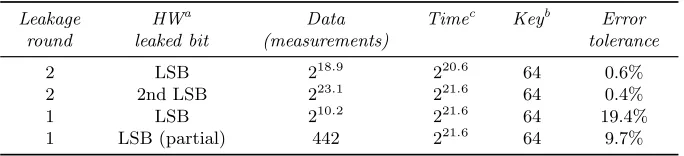
decoding becomes infeasible for PRESENT (n= 80). We solve this problem with a divide-and-conquer strategy. The results are summarized in Table 1.
Table 1.Simulation results on PRESENT under our BSC model
Leakage HWa Data Timec Keyb Error
round leaked bit (measurements) tolerance
2 LSB 218.9
220.6
64 0.6%
2 2nd LSB 223.1 221.6 64 0
.4%
1 LSB 210.2
221.6
64 19.4%
1 LSB (partial) 442 221.6 64 9
.7%
aHamming weight.
bNumber of key bits recovered. cNumber of key trials.
ET-SCCA based on the application to PRESENT. In Section 6 we compare ET-SCCA with other side-channel attacks and provide some countermeasures. Finally, we conclude the paper in Section 7.
2
Preliminaries
2.1 Cube and Side-Channel Cube Attacks
Cube attacks were introduced by Dinur and Shamir at Eurocrypt 2009 [8]. It is closely related to high-order differential attacks [18] and algebraic IV d-ifferential attacks [29][30]. The differences between cube attack and high order differential attack are elaborated in [12]. Cube attacks consist of two phases: the off-line phase and the on-line phase. The off-line phase determines which queries should be made to a cryptosystem during the on-line phase of the at-tack. It is performed once per cryptosystem. Note that the knowledge of the internal structure of the cipher is not necessary. In the on-line phase, attackers deduce a group of linear equations by querying the cryptosystem with tweakable public variables (e.g., chosen plaintexts). Finally, the attacker solves the linear equations to recover the secret key bits. We give a toy example below.
Consider a block cipherTand its encryption function (c1, ..., cm) = E(k1, ...,
kn, v1, ..., vm), whereci, kj andvs are ciphertext, encryption key and plaintext
bits, respectively. One can always represent ci, i ∈ [1, m], with a multivariate
polynomial in the plaintext and key bits, namely, ci = p(k1, ..., kn, v1, ..., vm).
The polynomialpis called amaster polynomialofci.
LetI⊆ {1, ..., m}be an index subset, andtI =Qi∈Ivi, the polynomialpis
divided into two parts:
p(k1, ..., kn, v1, ..., vm) =tI ·pS(I)+q(k1, ..., kn, v1, ..., vm),
where no item in qcontains tI. Here pS(I) is called the superpoly of I in p. A maxterm ofpis a termtI such that deg(pS(I))≡1, i.e., the superpoly ofI inp is a linear polynomial which is not a constant.
Example 1. Let p(k1, k2, k3, v1, v2, v3) = v2v3k1+v2v3k2 +v1v2v3+v1k2k3+ k2k3+v3+k1+ 1 be a polynomial of degree 3 in 3 secret variables and 3 public variables. Let I = {2,3} be an index subset of the public variables. We can representpasp(k1, k2, k3, v1, v2, v3) =v2v3(k1+k2+v1) + (v1k2k3+k2k3+v3+ k1+ 1),where
tI =v2v3,
pS(I)=k1+k2+v1,
q(k1, k2, k3, v1, v2, v3) =v1k2k3+k2k3+v3+k1+ 1.
Letdbe the size ofI, then acubeonIis defined as a setCI of 2d vectors that
cover all possible combinations oftI, while setting other public variables to be
constant. Any vector τ ∈ CI defines a new derived polynomial p|τ with n−d
CI results in exactlypS(I)(cf. Theorem 1, [8]). For pandI defined in Example 1, we haveCI ={τ1, τ2, τ3, τ4}, where
τ1= [k1, k2, k3, v1,0,0], τ2= [k1, k2, k3, v1,0,1],
τ3= [k1, k2, k3, v1,1,0], τ4= [k1, k2, k3, v1,1,1].
It is easy to verify thatp|τ1+p|τ2+p|τ3+p|τ4=k1+k2+v1=pS(I). HerepS(I) is called the maxterm equation oftI. In the off-line phase, the attacker tries to
find as many maxterms and their corresponding maxterm equations as possible. In the on-line phase, the secret key is fixed. The attacker chooses plaintexts τ ∈CI and obtains the evaluation of patτ. By summing up p|τi for all the 2
d
vectors in CI, the attacker obtains pS(I), a linear equation inki. The attacker
repeats this process for all the maxterms found in the off-line phase, and obtains a group of linear equations. If the number of independent equations is larger than or equal to n, the bit-length of the key, then the attacker can solve the linear equation system and recover the key.
2.2 Side-Channel Cube Attack
Side-channel cube attacks [10] use the knowledge about intermediate vari-ables (i.e., state registers) as the target bits, and consequently the evaluation of pis obtained through side-channel leakage. Since side-channel leakage is likely to contain noise, solving the linear equation system becomes a challenge. To tackle this problem, Dinur and Shamir proposed to use error correction code to remove the measurement errors. In the DS model, each measurement can have three possible outputs: 0, 1 and⊥, where⊥indicates the measurement cannot be relied upon. The attacker assigns a new variableyj to each⊥and computes
the maxterm equations. As a result, the maxterm equation has yj on the right
hand side. As for example 1, assuming the second measurement was not reliable, the obtained maxterm equation becomes k1+k2+v1 =p|τ1 +p|τ3+⊥+p|τ4. DS model replaces the ⊥in the maxterm equation with a new variableyi. As
a result, the equation becomes k1+k2+v1 =p|τ1+p|τ3+yi+p|τ4. For each cube, there might be new variable introduced. In order to solve this equations, additional measurements are required.
In the off-line phase, the attacker chooses a large cube of sizekand computes all the coefficients of all the d−k1
linear equations which are determined by summing over all the possible subcubes of dimensiond−1. In the on-line phase, the attacker obtains 2k leaked bits. Let ǫ be the fraction of the ⊥ among all
the measurements. Out of the 2k values,ǫ·2k values are⊥. It is assumed that
the errors are uniformly distributed and the leakage function is a d-random multivariate polynomial. More precisely, the definition ofd-random polynomial [8] is as follows.
Definition 1 A d-random polynomial withn+mvariables is a polynomialp∈
Letnbe the number of secret key variables. The attacker chooses a big cube with k ≥ d+ lognd public variables1. The attacker obtains a system of d−k1
linear equations in theǫ·2k+nvariablesy
j andki. As far as d−k1≥(ǫ·2k+n),
the attacker can solve the linear equations and obtain the key. The error ratioǫ should satisfy the following condition:
ǫ≤ k d−1
−n
2k . (1)
The attacker can thus find the key when at most ( k d−1)−n
2k fraction of the leaked bits are⊥. This model was further enhanced in [11] by using more trivial equa-tions of high dimension cubes to correct the errors. The number of measurements increased exponentially whenkincreases. Such a large amount of measurements is hard to obtain in side-channel analysis, especially in power analysis. Note that the success of this model is based on the assumption that the attacker knows which measurement is correct and which one is not. This is a strong assumption since in reality every measurement is likely to be noisy. In the following section, we consider a more practical model where each measurement is noisy.
3
A New Error-Tolerant Side-channel Cube Attack
Note that all the coefficients of maxterm equations can be obtained in the off-line phase. Suppose we can deriveLlinear equations in the off-line phase and the average cube size of all the corresponding maxterms is ¯d, then we have a linear equation system as follows:
l1: a1
1k1+a21k2+...+an1kn =b1
l2: a12k1+a22k2+...+an2kn =b2
.. .
lL: a1Lk1+a2Lk2+...+anLkn=bL
(2)
where aji ∈ {0,1} (1 ≤ i ≤ L,1 ≤ j ≤ n) denotes the coefficient of a linear
equation. Note that bi ∈ {0,1} is obtained by summing up the evaluation of
the maxterm equation over theith cubeCi, namely,bi=Pτ∈Cip|τ. The value ofp|τ is obtained via measurements. Ideally, the measurement is error-free and
the attacker obtains the correct sequenceB= [b1, b2, ..., bL]. In reality, however,
the attacker is likely to observe a different sequenceZ=z1, z2, ..., zLdue to the
measurement errors.
Letq be the probability that a bit may flip in each measurement. We can assumeq <1/2, then 1−q= 1/2 +µis the probability that we get an accurate measurement and µ= 0 means a random guess. Since bi =Pτ∈Cip|τ, andCi
1
we only need aboutd+logn
d tweakable public variables in order to packndifferent
maxterms among their products, since d+lognd d
hast = 2d¯elements, and each measurement can be treated as an independent
event, according to the piling-up lemma [16], we can derive
P r{bi=zi}= 1∆ −p=1
2 + 2
t−1µt. (3)
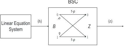
Thus, the observed sequenceZ=z1, z2, ..., zLcan be regarded as the received
channel output and the sequenceB=b1, b2, ..., bLis regarded as a codeword from
an [L, n] linear block code, whereL is the code length andnis the dimension. We can describe each zi as the output of the binary symmetric channel (BSC,
see Fig.1) withp= 1/2−ε(ε= 2t−1µt) being the crossover probability.
1-p
1-p
p
p
BSC
B Z
{bi} {zi}
Linear Equation System
Fig. 1.The error-tolerant side-channel attack model
Therefore, the key recovery problem is now converted to the problem of decoding a [L, n] linear code. Let H(x) = −xlog2x−(1 −x)log2(1−x) be the binary entropy function, if the code rate R=n/Lis less than the capacity C(p) = 1−H(p), then in the ensemble of random linear [L, n] codes, the decoding error probability approaches zero. Various decoding techniques can be adopted to recover the secret key.
4
Decoding Algorithms
4.1 Maximum Likelihood decoding (ML-decoding)
Siegenthaler [28] firstly proposed the use of ML-decoding in cryptanalysis of a stream cipher by exhaustively searching through all the codewords of the above [L, n]-code. The complexity of this algorithm is aboutO(2n·n/C(p)). We
give a brief introduction of ML-decoding below.
LetA= (aji)L×n (1≤i≤L,1≤j ≤n) be the generator matrix of (2) and
Ai denote thei-th row vector ofA. The aim of the decoding is to find the closet
codeword (b1, b2, ..., bL) to the received vector (z1, z2, ..., zL), and decode the key
variablesk= (k1, k2, ..., kn) such that bi=k·ATi, whereT denotes the matrix
transpose, i.e., find suchkthat minimizes D(k) =PLi=1(ziLbi).
Simulations [28] show that the critical lengthL=l0≈0.35·n·ε−2provides the probability of successful decoding close to 1/2, while forL= 2l0the probability is close to 1.
4.2 Error Probability Evaluation
In our model, we can get the following theorem on the theoretical relationship.
Theorem 1 If we deriveL linear equations containing nkey variables and the
average cube size of all the corresponding maxterms isd¯, then we can recover all the n key bits with success probability close to50%when the error probability q
of each measurement satisfies
q≤ 1
2 ·(1−( 0.35·n
L )
1 2·t ·2
1
t), (4)
wheret= 2d¯denotes the number of summations to evaluate each linear equation.
Proof. In order to have a probability of successful decoding close to 1/2 us-ing the ML-decodus-ing, the code length L should be larger than 0.35·n·ε−2, that is L ≥ 0.35·n·ε−2. Thus we get ε ≥ q0.35·n
L . Since ε = 2t−1µt
hold-s, then we can derive µ ≥(0.35·n L )
1 2·t ·2
1
t−1. From q = 1/2−µ, we have q ≤ 1
2·(1−( 0.35·n
L )
1 2·t ·2
1
t).
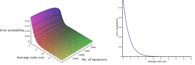
Suppose the number of key variables is n = 80, the error probability is depicted in the following figure.
Fig. 2. Error probability q as a func-tion of ¯dandL(Givenn= 80)
Fig. 3. Error probability q as a func-tion of ¯d(GivenL= 1000,n= 80)
Under the assumption that the master polynomial is ad-random multivariate polynomial, L = d−k1
linear equations (containing n key variables) can be derived with the corresponding maxterm size ofd−1. Then we get the following corollary.
Corollary 1 If the master polynomial is a d-random multivariate polynomial
and we choose a big cube withk≥d+lognd public variables, then we can recover all the nkey bits with success probability close to50%when the error probability
q of each measurement satisfies
q≤ 1
2 ·(1−( 0.35·n
k d−1
)
1 2·t ·2
1
t), (5)
where t = 2d−1 denotes the number of summations to evaluate each maxterm
equation.
4.3 Improving the Success Rate and Decoding Complexity
When applying side-channel cube attacks to a specific cryptosystem, the number of linear equations we can derive might be limited. In other words, the code lengthL may not be big enough to reach a high probability of successful decoding. In this case, the decoding algorithm is likely to output wrong key which is not far from the correct key. To overcome this problem, we output a list of candidates and verify each one using a valid plaintext/ciphertext pair.
Whennbecomes larger, the ML-decoding process becomes expensive since it has a time complexity of 2n. This problem can be solved if the linear equations
can be divided into almost disjoint sets. We first divide the set{k1, k2, ..., kn}
in-toηgroupsG1, G2, ..., Gη, each with roughly⌈n/η⌉key variables. For each group
Gi, we collect those linear equations only containing the secret variables inGi.
The ML-decoding in each Gi has a complexity of O(2⌈n/η⌉· ⌈n/η⌉/C(p)). Note
that the linear equations are likely to be sparse, which makes the splitting strat-egy easy to apply. Previous study on Trivium [8], Serpent [11, 10] and KATAN [15] shows that the linear equations generated by cube attacks are indeed sparse. Note that the ML-decoding is not the only decoding algorithm of linear binary codes. In fact, since most of the linear equations derived from the cube summations have a low density, other decoding algorithms [31, 14, 21, 6] that exploit this properties may achieve better results. We do not claim to be experts in the design and usage of coding. However, in this study, we want to highlight the importance of the procedure of transforming the side-channel cube attack within noise leakage to the decoding of a binary linear code.
5
Evaluation of our ET-SCCA on PRESENT
5.1 Hamming Weight Leakage
Like previous attacks [25, 23, 26], we assume the PRESENT cipher is imple-mented on a 8-bit processor. The attacker exploits the hamming weight leakage when the intermediate variables (state variables) are loaded from the memory to the ALU. Let wH(x) be the Hamming weight function which outputs the
number of 1s in x. Let S = {s0, s1, ..., s7} be a 8-bit internal state, then the value of wH(S) can be represented with a 4-bit valueH ={h0, h1, h2, h3} and
h0 denotes the least significant bit (LSB) and h3 denotes the most significant bit (MSB). Each hi, 0 ≤i ≤3 can be calculated2 as h0 =P7i=0si, h1 = P
(0≤i<j≤7)sisj, h2 = P(0≤i<j<m<l≤7)sisjsmsl, h3 = Q7i=0si. From
the expression of eachhi, the algebraic degree increases from LSB to MSB and
eachhi contains all the 8 internal state bits.
5.2 Cube Searching Strategy
The cube searching strategy in our attacks is as follows. We keep two types of monomials for each round, one involving a single key variable and the other only involving public variables. Then in the next round we compute the terms in the polynomial of the state bit which are related to the selected terms only. And we discard other terms involving more than one key variables. In this way, we can explicitly compute the multivariate polynomials in the key variables and plaintext variables for each state bit in the first few rounds of PRESENT and treat the coefficient of the linear terms and constant terms as cubes.
5.3 Simulations on the Second Round
As shown above, in order to have a high error tolerance rate, the cube size should not be too big. We start with by attacking the second round. The internal state contains 8 bytes denoted bybyte1, byte2, ..., byte8. In the off-line phase, we have searched each state byte using our cube searching strategy. If the LSB of the Hamming weight of byte8 after the second round is leaked, we can in total obtainL= 2232 linear equations containing 64-bit key variables. The problem of recovering those 64-bit key is now equivalent to the problem of decoding a [2232,64] linear code.
Since a direct application of the ML-decoding algorithm has a time com-plexity of 264, we divide all the key variables into 4 groupsG1, G2, G3 andG4 and apply the ML-decoding in each group. To ensure the success probability, we save a candidate list of T closest solutions for each group. However, the num-ber of candidates becomesT4, leading to an expensive verification step. A more efficient way is to use overlapping groups where each group shares with neigh-boring groups with 3-4 key bits. Now we only have to verify the combination of candidates that agree in the overlapping bits, which can reduce the number of verifications by a factor of about 29to 212.
2 All the summations are based on finite field
The grouping strategy here is to keep the code rate of each group as low as possible by utilizing the sparse structure of the linear maxterm equations, since it can further accelerate the decoding phase and the verification phase. Table 2 shows the configurations of the 4 groups and their overlapping bits.
Table 2.Groups on the LSB of the Hamming weight of
byte8
Group [L, n] Key bits Overlapping bits
G1 [690,19] [k17, k18, ..., k35] 3 withG2
G2 [690,19] [k33, k34, ..., k51] 3 withG1, 3 withG3
G3 [690,19] [k49, k50, ..., k67] 3 withG2, 3 withG4
G4 [558,16] [k65, k66, ..., k80] 3 withG3
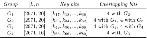
Using the same strategy, we also group the key variables in all theL= 10468 maxterm equations containingn= 64 key variables on the attack of the second LSB leakage of the Hamming weight of byte1. The configurations are listed in Table 3.
Table 3.Groups on the 2nd LSB of the Hamming weight
ofbyte1
Group [L, n] Key bits Overlapping bits
G1 [2971,20] [k17, k18, ..., k36] 4 withG2
G2 [2971,20] [k33, k34, ..., k52] 4 withG1, 4 withG3
G3 [2971,20] [k49, k50, ..., k68] 4 withG2, 4 withG4
G4 [2671,16] [k65, k66, ..., k80] 4 withG3
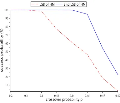
Under these configurations, we have simulated the decoding algorithm for 100 runs withT= 200. For each run, we randomly generate a key and construct the linear code in each group. The noise was simulated by a random binary number generator according to the crossover probabilityp(e.g., supposek0 = 1, k1= 0 and there is a linear equation 1 +k0+k1=zi, the value ofzi will flip to 1 with
probabilitypand remain unchanged with probability 1−p). We have conducted the simulation for 10 times and the average number of successful decoding out of a batch of 100 runs are recorded. The simulation results with various crossover probability are given in Fig.4.
From Fig.4, with the crossover probabilityp = 0.44, the decoding success probability of the LSB leakage ofbyte8 is 61.10%. Whenp= 0.47, the decoding success probability of the 2nd LSB leakage ofbyte1is 54.10%. Due to the lower code rate, the decoding success probability of 2nd LSB leakage is relatively higher than that of the LSB leakage.
Fig. 4.Simulation results of list decoding
Table 4.Noise level under different leakage positions
HW Leakage Round p Average cube q
position sized
LSB (byte8) 2 44% 7.7 0.6% 2nd LSB (byte1) 2 47% 8.4 0.4%
The whole attack contains two phases, the first phase is the decoding in each group. The results in this phase are the candidate lists. Letti denote the time
complexity of decoding in group Gi, m denote the number of the groups and
ni denote the code dimension inGi, thus the time complexity in this phase is Pm
i=1tiwhereti= 2ni key trials. The second phase is the verification phase, the
time complexity in this phase is Q(T) =Tm/2r encryptions, where T denotes the size of candidate list and 2r is the reduction factor. Therefore, the total
attack complexity is bounded bymax{Pmi=1ti, Tm/2r}. The attack results on
PRESENT are given in Table 5.
Table 5. Attack results on PRESENT
Leakage Timeb Memory Data r Success Error
position requirementa (measurements) probability probability
LSB 220.6
3 KB 218.9
9 61.1% 0.6%
2nd LSB 221.6 3 KB 223.1 12 54
.1% 0.4%
It is clear to see that we can have an average successful probability of 61.1% to restore 64 key bits with a time complexity of 220.6, negligible memory re-quirement and q = 0.6% error probability for each measurement. The rest 16 key bits can be exhaustively searched. Although the BSC model can tolerant noise in each measurement, the error tolerances are very low. The reason is that the cube size in the second round is relatively big. The bigger cube size will lead to an exponential increase oftin equation (3). Thus the error probabilityq become very low. In the following section, we evaluate the model based on the leakage of the first round, which shows better results.
5.4 Simulation on the first round
The diffusion of the first round is far from complete, thus we need to utilize more leaked bits instead of a single one to ensure the decoding success proba-bility. Using our cube searching, we derived all the possible cubes from the LSB leakage of all the 8 bytes:byte1, byte2, ..., byte8 after the first round. Then we perform the off-line phase by utilizing all those cubes and obtained hundreds of maxterm equations (see Appendix B). According to the key variables distribu-tion in these maxterm equadistribu-tions, all the 8 bytes can be classified into 2 classes in Table 6.
Table 6.Classification of state bytes after the first round
Class State byte Key No. of maxterm Average variablesa equations cube size
Class1 byte1, byte3, byte5, byte7 k17, k18, ..., k48 150 1.90
Class2 byte2, byte4, byte6, byte8 k49, k50, ..., k80 152 1.89
aThe number of key variables for both classes are 32.
From Table 6, the average cube size for both classes are relatively smaller than that of the second round. The grouping strategy is the same to that described in section 5.2. We combineClass1 andClass2and divide them into 4 groups in Table 7.
Table 7. Groups on the LSB of the Hamming weight
after the first round
Group [L, n] Key bits Overlapping bits
G1 [93,20] [k17, k18, ..., k36] 4 withG2
G2 [95,20] [k33, k34, ..., k52] 4 withG1, 4 withG3
G3 [95,20] [k49, k50, ..., k68] 4 withG2, 4 withG4
G4 [76,16] [k65, k66, ..., k80] 4 withG3
the average number of successful cases. Results show that when p = 42% the decoding success probability is 50.1%. Thus the error probability of each mea-surement is q = 19.4%. The results are summarized in the following Table 8.
Table 8.ET-SCCA on the first round
Leakage Timeb Memory Data
r Success Error position requirementa (measurements) probability probability
LSB 221.6
3 KB 210.2
12 50.1% 19.4%
a4 candidate lists of 4·200 entries, with each entry of 4 bytes. bThe number of key trials.
Compared to the attack on the second round, a higher error probability is achieved based on the leakage of the LSB of the state bytes after the first round. We can have a success probability of 50.1% to recover all the 64 master key bits diffused in the first round with time complexity of 221.6, negligible memory requirement and 210.2 data complexity, when the error probability of each mea-surement is at most 19.4%. We can further reduce the data complexity to 442 by utilizing partial leaked bits after the first round, while the error tolerance level also reduced to about 9.7% accordingly (see Appendix B for details). The data complexity (measurements) in our estimation is the upper bound, since when we target on the multiple bytes in the first round, we can reduce the measurements by reusing the duplicate cubes.
Note that the time complexity can be further reduced by splitting the max-terms into more groups with similar size to each other. Thus the cost for decoding can be reduced, while the number of candidates increases (we can also reduce the time complexity of verification phase by introducing more overlapping bits) and the decoding success probability and error probability may also change accord-ingly. There is a tradeoff between time, success probability and error probability. We do not claim that our grouping is optimal as there may be better choices.
The simulation result demonstrates that the cube size has a great influence on the error tolerance level, which is consistent with our previous analysis. To maximize the efficiency, one should apply the attack to the early rounds of a cipher, in which the algebraic degree of the state is relatively low. Even though we may derive more maxterms in the later round to gain a higher crossover probability p for each equation, the error probability q for each measurement will drop very quickly due to the higher cube size.
6
Comparison and Discussion
the error-correction strategy is also different. We regard the key recovery prob-lem as the decoding of some linear codes transmitted through the BSC, while the DS model considers it as erasure codes.
Note that the DS model performs 2k measurements, while our model
per-forms less than L·2d¯measurements. For both models, the number of traces
grows exponentially when the cube size goes up. The DS model targets the leak-age round where a complete diffusion is achieved [11]. Taking PRESENT as an example, after three rounds,dis around 20. Thus, to maximize the error toler-ance according to (1),kshould be roughly 40. The attacker needs to perform 240 measurements, which is order of magnitude larger than that of standard DPA.
The original algebraic side-channel attack (ASCA) [25, 26] is sensitive to measurement noise and the theoretical estimates of the attack complexities are hard to derive. In addition, a large number of leakage information is required when feeding the Biryukov-Canni`ere system [3] into the algebraic solvers. This attack was later improved by Orenet al.[23] to handle more noisy leakage. They consider the key recovery problem as a pseudo-Boolean optimization (PBOPT) problem. However, a theoretic estimation of the error tolerance is missing. The ASCA exploits multiple information leakage on a single power trace, while the side-channel cube attack uses leakage from a single wire in many executions. The ASCA also claims to be able to break masked implementations, while it is not clear yet if ET-SCCA can also break masking.
In order to prevent side-channel cube attack, the design should add more noise to increase the probability of measurement errors. Many known techniques can be used here.
– Noise generation. The noise generator actively flattens the power trace with noise.
– Dual-rail logic. Dual-rail logic hides data-dependent flips inside the combi-national logic and registers. It helps to reduce the signal-to-noise ratio. – Data-bus encryption. When the bus between the ALU and memory is
en-crypted, it is more difficult for the attackers to obtain the hamming weight of the data.
– Random execution order. The order of internal operations (e.g. substitution) in each round can be randomized. It becomes more difficult for the attackers to locate the leakage of the target bit.
Note that countermeasures listed above are originally designed to thwart power analysis. If the EM analysis is used, some of this countermeasures may be inef-fective. For example, noise generation is not likely to prevent EM analysis that uses only local EM leakage.
7
Conclusion and Open Problems
decoding a linear code. We analyzed the error tolerance capacity of the new model and verified the model using PRESENT. We also observed that since the encoding matrix is sparse, it’s possible to speed up the decoding process using a divide-and-conquer strategy. Our simulation results on PRESENT show that given about 210.2 measurements, each with an error probability of 19.4%, our model achieves 50.1% of success rate for the key recovery.
The study of side-channel cube attack is still at its early age. Here we list several open problems.
1. How to select the best target bit and find more maxterm equations. The current random walk method is very time-consuming.
2. Can side-channel cube attacks break masked implementations? 3. How to increase the error tolerance efficiently?
4. When using BSC model, can we speed up the decoding process further by exploiting the sparse structure of the encoding matrix?
References
1. Aumasson, J.-P., Dinur, I., Meier, W., Shamir, A.: Cube Testers and Key Recovery Attacks on Reduced-Round MD6 and Trivium. In: Dunkelman, O. (Ed.): Fast Software Encryption-FSE’2009, LNCS, vol. 5665, pp. 1-22. Springer, Heidelberg (2009)
2. Aumasson, J.-P., Dinur, I., Henzen, L., Meier, W. and Shamir, A.,: Efficient FP-GA implementations of high-dimensional cube testers on the stream cipher Grain-128.Special Purpose Hardware for Attacking Cryptographic Systems-SHARCS’09’. (2009)
3. Biryukov, A., De Canni`ere, C. : Cryptanalysis of Block Ciphers with Overdefined Systems of Equations. Fast Software Encryption-FSE’2003, LNCS, vol. 2887, pp. 274-289. Springer, Heidelberg (2003)
4. Blum, M., Luby, M., Rubinfeld, R.: Self-testing/correcting with applications to numerical problems.Journal of Computer and System Sciences47, 549-595 (1993) 5. Bogdanov, A., Knudsen, L., Leander, G., Paar, C., Poschmann, A., Robshaw, M., Seurin, Y., Vikkelsoe, C.: PRESENT: An ultra-lightweight block cipher. In: Pail-lier, P., Verbauwhede, I. (eds.): Cryptographic Hardware and Embedded Systems-CHES’2007, LNCS, vol. 4727, pp. 450-466. Springer, Heidelberg (2007).
6. Chung, S.-Y., Forney, G. D., Richardson, T., Urbanke, R.: On the design of low-density parity-check codes within 0.0045 dB of the Shannon limit.IEEE Commu-nications Letters, vol. 5, no. 2, pp. 58-60, Feb. (2001)
7. Courtois, N., Pieprzyk, J.: Cryptanalysis of Block Ciphers with Overdefined Sys-tems of Equations. In: Zheng, Y. (ed.):Progress in Cryptology-ASIACRYPT’2002, LNCS, vol. 2501, pp. 267-287. Springer, Heidelberg (2002)
8. Dinur, I., Shamir, A.: Cube Attacks on Tweakable Black Box Polynomials. In: Joux, A. (ed.): Progress in Cryptology-EUROCRYPT’2009, LNCS, vol. 5479, pp. 278-299. Springer, Heidelberg (2009)
9. Dinur, I., Shamir, A.: Breaking Grain-128 with Dynamic Cube Attacks. In: Joux, A. (ed.):Fast Software Encryption-FSE’2011, LNCS, vol. 6733, pp. 167-187. Springer, Heidelberg (2011)
11. Dinur, I., Shamir, A.: Generic Analysis of Small Cryptographic Leaks. 2010 Work-shop on Fault Diagnosis and Tolerance in Cryptography. pp. 39-48. (2010) 12. Dinur, I., Shamir, A.: Applying cube attacks to stream ciphers in realistic scenarios.
Cryptography and Communications. no. 4, pp. 217-232. (2012)
13. Farebrother, R.W.: Linear Least Squares Computations.STATISTICS: Textbooks and Monographs, Marcel Dekker, ISBN 978-0-8247-7661-9, (1988)
14. Gallager, R.G.: Low-density parity-check codes.IRE Transactions on Information Theory, vol. IT-8, no. 1, pp. 21-28, Jan. (1962)
15. Gregory V.B., Nicolas T.C., Jorge N.J., Pouyan S., Bingsheng Z.: Algebraic, AI-DA/Cube and Side Channel Analysis of KATAN Family of Block Ciphers. In Gong G., Gupta K.C. (Eds.):Progress in Cryptology - INDOCRYPT 2010, vol.6498, pp. 176-196. Springer, Heidelberg (2010)
16. Matsui, M.: Linear Cryptanalysis Method for DES Cipher. In: Santis, A. D. (ed.): Progress in Cryptology-EUROCRYPT’1994, LNCS, vol. 765, pp. 386-379. Springer, Heidelberg (1994)
17. Kocher, P., Jaffe, J., Jun, B.: Differential power analysis. In: Wiener, M. (ed.): Progress in Cryptology-CRYPTO’99, LNCS 1666, pp. 388-397. (1999)
18. Lai, X.: Higher Order Derivatives and Differential Cryptanalysis.Communications and Cryptography: Two Sides of One Tapestry, 227 (1994)
19. Lin Yang, Meiqin Wang, and Siyuan Qiao.: Side Channel Cube Attack on PRESENT. In Garay, J.A., Miyaji A., Otsuka, A. (eds.):Cryptology and Network Security-CANS’2009, LNCS 5888, pp. 379-391. Springer, Heidelberg (2009) 20. Luby, M. G., Mitzenmacher, M., Shokrollahi, M. A., Spielman, D. A.: Efficient
erasure correcting codes. IEEE Transactions on Information Theory, vol. 47(2), pp. 569-584 (2001)
21. MacKay, D.: Good error correcting codes based on very sparse matrices. IEEE Transactions on Information Theory, vol. 45, no. 2, pp. 399-431, Mar. (1999) 22. Kocher, P.: Timing Attacks on Implementations of Diffie-Hellman, RSA, DSS, and
Other Systems. In Koblitz, N. (ed.):Progress in Cryptology-CRYPTO’96, LNCS 1109, pp.104-113. (1996)
23. Oren, Y., Kirschbaum, M., Popp, T., Wool, A.: Algebraic Side-Channel Analysis in the Presence of Errors. In: Mangard, S., Standaert, F.-X. (eds): Cryptograph-ic Hardware and Embedded Systems-CHES’2010, vol.6225, pp. 428-442. Springer, Heidelberg (2010)
24. Quisquater, J. J., Samyde, D.: A new tool for non-intrusive analysis of smart cards based on electro-magnetic emissions: the SEMA and DEMA methods[EB/OL]. Eurocrypt rump session. (2000)
25. Renauld, M., Standaert, F.-X.: Algebraic Side-Channel Attacks, Cryptology ePrint Archive, report 2009/179, http://eprint.iacr.org/2009/279. (2009)
26. Renauld, M., Standaert, F.-X., VeyrCharvillon, N.: Algebraic side-channel at-tacks on the AES: why time also matters in DPA. In: Clavier, C., Gaj, K. (Eds): Cryptographic Hardware and Embedded Systems-CHES’2009, vol.5747, pp. 97-111. Springer, Heidelberg (2009)
27. Shekh Faisal A-L., Mohammad R.R., Willy S., Jennifer S.: Extended Cubes: En-hancing the cube attack by Extracting Low-Degree Non-linear Equations. In Bruce C., Lucas C.K.H., Ravi S., Duncan S.Wong (eds.):ACM Symposium on Informa-tion, Computer and Communications Security-ASIACCS’2011, pp.296-305. (2011) 28. Siegenthaler, T.: Decrypting a class of stream ciphers using ciphertext only.IEEE
Transactions on Computers, vol. C-34, pp. 81-85. (1985)
30. Vielhaber, M.: AIDA Breaks (BIVIUM A and B) in 1 Minute Dual Core CPU Time. IACR Cryptology ePrint Archive, 402 (2009)
31. Wiberg, N.: Codes and decoding on general graphs. Ph.D. dissertation. Link¨oping University, Link¨oping, Sweden, (1996)
32. Zhao X.J., Wang T., Guo S.Z.: Improved Side Channel Cube Attacks on PRESENT. Cryptology ePrint Archive. Report 2011/165 (2011)
A
Reducing Data complexity
We can further reduce the data complexity by utilizing the partial leaked bits after the first round listed in the following Table 9.
Table 9.Classification of partial state bytes after the first round
Class State byte Key No. of maxterm Average variablesa equations cube size
Class3 byte1, byte3 k17, k18, ..., k48 62 1.70
Class4 byte2, byte4 k49, k50, ..., k80 64 1.75
aThe number of key variables for both classes are 32.
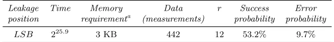
Using the same grouping strategy described in section 5.3, the attack results are summarized in the following Table 10.
Table 10.ET-SCCA on the first round
Leakage Time Memory Data r Success Error position requirementa (measurements) probability probability
LSB 225.9
3 KB 442 12 53.2% 9.7%
a4 candidate lists of 4·200 entries, with each entry of 4 bytes.
These results demonstrate that we can further reduce the data complexity to 442. Since we only utilize the partial leaked information to decode, the error probability also reduced.
Table 11. 150 maxterms and maxter-m equations obtained fromaxter-m the LSB of byte1, byte3, byte5, byte7
Cube Maxterm Cube Maxterm
Indexes equations indexes equations {2} k19 {3} 1 +k18
{6} k23 {7} 1 +k22
{11} 1 +k26 {14} k31
{15} 1 +k30 {18} k35
{19} 1 +k34 {22} k39
{23} 1 +k38 {26} k43
{27} 1 +k42 {30} k47
{31} 1 +k46 {1,3} k18 +k20
{1,4} k18 +k19 {2,3} k17
{2,4} 1 +k17 {3,4} 1 +k17
{5,6} k23 +k24 {5,7} k22 +k24
{5,8} k22 +k23 {6,7} k21
{6,8} 1 +k21 {7,8} 1 +k21
{1,2} 1 +k20 {1,3} k20
{1,4} 1 +k18 +k19 {2,4} 1 +k17
{3,4} k17 {5,6} 1 +k24
{5,7} k24 {5,8} 1 +k22 +k23
{6,8} 1 +k21 {7,8} k21
{1,2} k19 +k20 {1,3} k18 +k20
{1,4} k18 +k19 {2,3} 1 +k17
{2,4} k17 {3,4} k17
{5,6} k23 +k24 {5,7} k22 +k24
{5,8} k22 +k23 {6,7} 1 +k21
{6,8} k21 {7,8} k21
{9,10} k27 +k28 {9,11} k26 +k28
{9,12} k26 +k27 {9,10} 1 +k28
{9,11} k28 {9,12} 1 +k26 +k27
{9,10} k27 +k28 {9,11} k26 +k28
{9,12} k26 +k27 {10,11} k25
{10,12} 1 +k25 {11,12} 1 +k25
{13,14} k31 +k32 {13,15} k30 +k32
{13,16} k30 +k31 {14,15} k29
{14,16} 1 +k29 {15,16} 1 +k29
{17,18} k35 +k36 {17,19} k34 +k36
{17,20} k34 +k35 {18,19} k33
{18,20} 1 +k33 {19,20} 1 +k33
{21,22} k39 +k40 {21,23} k38 +k40
{21,24} k38 +k39 {22,23} k37
{22,24} 1 +k37 {23,24} 1 +k37
{25,26} k43 +k44 {25,27} k42 +k44
{25,28} k42 +k43 {26,27} k41
{26,28} 1 +k41 {27,28} 1 +k41
{29,30} k47 +k48 {29,31} k46 +k48
{29,32} k46 +k47 {30,31} k45
{30,32} 1 +k45 {31,32} 1 +k45
{10,12} 1 +k25 {11,12} k25
{13,14} 1 +k32 {13,15} k32
{13,16} 1 +k30 +k31 {14,16} 1 +k29
{15,16} k29 {17,18} 1 +k36
{17,19} k36 {17,20} 1 +k34 +k35
{18,20} 1 +k33 {19,20} k33
{21,22} 1 +k40 {21,23} k40
{21,24} 1 +k38 +k39 {22,24} 1 +k37
{23,24} k37 {25,26} 1 +k44
{25,27} k44 {25,28} 1 +k42 +k43
{26,28} 1 +k41 {27,28} k41
{29,30} 1 +k48 {29,31} k48
{29,32} 1 +k46 +k47 {30,32} 1 +k45
{31,32} k45 {10,11} 1 +k25
{10,12} k25 {11,12} k25
{13,14} k31 +k32 {13,15} k30 +k32
{13,16} k30 +k31 {14,15} 1 +k29
{14,16} k29 {15,16} k29
{17,18} k35 +k36 {17,19} k34 +k36
{17,20} k34 +k35 {18,19} 1 +k33
{18,20} k33 {19,20} k33
{21,22} k39 +k40 {21,23} k38 +k40
{21,24} k38 +k39 {22,23} 1 +k37
{22,24} k37 {23,24} k37
{25,26} k43 +k44 {25,27} k42 +k44
{25,28} k42 +k43 {26,27} 1 +k41
{26,28} k41 {27,28} k41
{29,30} k47 +k48 {29,31} k46 +k48
{29,32} k46 +k47 {30,31} 1 +k45
{30,32} k45 {31,32} k45
Table 12. 152 maxterms and
maxter-m equations obtained fromaxter-m the LSB of byte2, byte4, byte6, byte8
Cube Maxterm Cube Maxterm
Indexes equations indexes equations {34} k51 {35} 1 +k50
{38} k55 {39} 1 +k54
{42} k59 {43} 1 +k58
{46} k63 {47} 1 +k62
{50} k67 {51} 1 +k66
{54} k71 {55} 1 +k70
{58} k75 {59} 1 +k74
{62} k79 {63} 1 +k78
{33,34} k51 +k52 {33,35} k50 +k52
{33,36} k50 +k51 {34,35} k49
{34,36} 1 +k49 {35,36} 1 +k49
{37,38} k55 +k56 {37,39} k54 +k56
{37,40} k54 +k55 {38,39} k53
{38,40} 1 +k53 {39,40} 1 +k53
{41,42} k59 +k60 {41,43} k58 +k60
{41,44} k58 +k59 {42,43} k57
{42,44} 1 +k57 {43,44} 1 +k57
{45,46} k63 +k64 {45,47} k62 +k64
{45,48} k62 +k63 {46,47} k61
{46,48} 1 +k61 {47,48} 1 +k61
{49,50} k67 +k68 {49,51} k66 +k68
{49,52} k66 +k67 {50,51} k65
{50,52} 1 +k65 {51,52} 1 +k65
{53,54} k71 +k72 {53,55} k70 +k72
{53,56} k70 +k71 {54,55} k69
{54,56} 1 +k69 {55,56} 1 +k69
{57,58} k75 +k76 {57,59} k74 +k76
{57,60} k74 +k75 {58,59} k73
{58,60} 1 +k73 {59,60} 1 +k73
{61,62} k79 +k80 {61,63} k78 +k80
{61,64} k78 +k79 {62,63} k77
{62,64} 1 +k77 {63,64} 1 +k77
{33,34} 1 +k52 {33,35} k52
{33,36} 1 +k50 +k51 {34,36} 1 +k49
{35,36} k49 {37,38} 1 +k56
{37,39} k56 {37,40} 1 +k54 +k55
{38,40} 1 +k53 {39,40} k53
{41,42} 1 +k60 {41,43} k60
{41,44} 1 +k58 +k59 {42,44} 1 +k57
{43,44} k57 {45,46} 1 +k64
{45,47} k64 {45,48} 1 +k62 +k63
{46,48} 1 +k61 {47,48} k61
{49,50} 1 +k68 {49,51} k68
{49,52} 1 +k66 +k67 {50,52} 1 +k65
{51,52} k65 {53,54} 1 +k72
{53,55} k72 {53,56} 1 +k70 +k71
{54,56} 1 +k69 {55,56} k69
{57,58} 1 +k76 {57,59} k76
{57,60} 1 +k74 +k75 {58,60} 1 +k73
{59,60} k73 {61,62} 1 +k80
{61,63} k80 {61,64} 1 +k78 +k79
{62,64} 1 +k77 {63,64} k77
{33,34} k51 +k52 {33,35} k50 +k52
{33,36} k50 +k51 {34,35} 1 +k49
{34,36} k49 {35,36} k49
{37,38} k55 +k56 {37,39} k54 +k56
{37,40} k54 +k55 {38,39} 1 +k53
{38,40} k53 {39,40} k53
{41,42} k59 +k60 {41,43} k58 +k60
{41,44} k58 +k59 {42,43} 1 +k57
{42,44} k57 {43,44} k57
{45,46} k63 +k64 {45,47} k62 +k64
{45,48} k62 +k63 {46,47} 1 +k61
{46,48} k61 {47,48} k61
{49,50} k67 +k68 {49,51} k66 +k68
{49,52} k66 +k67 {50,51} 1 +k65
{50,52} k65 {51,52} k65
{53,54} k71 +k72 {53,55} k70 +k72
{53,56} k70 +k71 {54,55} 1 +k69
{54,56} k69 {55,56} k69
{57,58} k75 +k76 {57,59} k74 +k76
{57,60} k74 +k75 {58,59} 1 +k73
{58,60} k73 {59,60} k73
{61,62} k79 +k80 {61,63} k78 +k80
{61,64} k78 +k79 {62,63} 1 +k77