MODELLING OF FIRE SPREAD
AND THE GROWTH OF FIRE IN BUILDINGS
USING
COMPUTATIONAL FLUID DYNAMICS
ANTHONY ERNEST FERNANDO
A research thesis completed as fulfilment of the requirements of the degree
Doctor of Philosophy
undertaken at the
Centre for Environmental Safety and Risk Engineering
Victoria University of Technology
2000
Illl^Z
WER THESIS
ACKNOWLEDGMENTS
Five and a half years ago, I undertook a life altering journey, the culmination of which is the substantial wad of processed wood pulp the reader is presently either holding in their hand or (more likely) lain prone upon a sturdy surface. Like most such pieces of work, there are many forces at work in its creation other than the author's quill (or in this case, mouse and keyboard), and I would like to acknowledge these persons or organisations here.
The research presented in this thesis was financially supported by an Australian Research Council (ARC) Infrastructure Grant which was conducted in association with BHP and the National Association of Forest Industries. My gratitude to these organisations for making this research possible.
I would like to thank my principal supervisor. Professor Vaughan Beck, Director of the Centre for Environmental Safety and Risk Engineering, for taking me on as a student and choosing the area of research. He was a source of good advice on the writing of conference papers and this thesis, although his pen had a seemingly endless supply of red ink. I would also like to thank my co-supervisor, Associate Professor Graham Thorpe, for helping to explain some of the more technical and numerical aspects of the work in this project, and for likewise being adept with the crimson writing fluid. My gratitude to my other co-supervisor, Dr. Mingchun Luo, who was the resident expert on the field model CESARE-CFD, and helped to explain some of the quirks of this most complex beast. This thesis would also not have been possible without the clear-headed advice of Dr. Ozden Turan, who was also a great help in unravelling the mysteries (for me, anyway) of the k-epsilon turbulence model. My thanks also to Dr. Yaping He, Mr. Paul Clancy, and Mr. Mahesh Prakash, who have helped with other technical aspects of this thesis.
There was a substantial amount of work involved in the preparation and execution of experiments at the Experimental Building Fire Facility. My gratitude to Mr. Scott Stewart for setting up the instrumentation and doing all the hard work in preparing the facility for testing. He was assisted by Messrs. Eddie Szmaiko and Ben White for the propane burner tests, and Martin Coles for the polyurethane foam tests. My thanks to all these persons.
completing the .second round of cone calorimeter tests. Vince was also responsible for organising the furniture calorimeter tests which were ably carried out by Messrs. Neville Macarthur and Alex Webb.
On a personal note, I would like to thank family and friends who have been so sympathetic and supportive the last four years. In particular, I wish to express my gratitude to my "-in-laws" Derrick and Rita Fernando for their encouragement, generosity, and weekly curries, and Rosie Fernando and Trevor Plant for their support and friendship. I would also like to thank Trevor for his "expertise" in setting up my home computer, for frequent loans of his zip drive, and for insisting I upgrade my home computer (a worthwhile investment as it transpires, although the result is that I now own the PC equivalent of the Millennium Falcon). My thanks to Evan Linwood for musical distractions on nights off, and also for providing the frame-grabber technology and producing the video stills for the thesis. My thanks also to my friends Grant Armstrong, who started his PhD six months before me, and Iain and Luisa Cook, who completed theirs several years ago, for their sympathy, wisdom and advice, having been through it all themselves.
I would dearly like to thank my grandmother, Lilian Leitch (1/7/13 - 16/6/98) who provided me with companionship and a home during my undergraduate years, and also frequently provided a nice hot cuppa and a stress-free zone during my postgraduate years. "Gran" is still missed by all.
ABSTRACT
The motivation for undertaking this research is to contribute to the development of a model of fire spread over a surface, and to integrate this model with a computational fluid dynamics (CFD) model that is capable of making predictions of the environment associated with full-scale fires in enclosures. The research focuses on the growth and spread stage of such fires, where a small, localised flame spreads across a single fuel item, increasing the heat release rate. In particular, the phenomenon of opposed flow flame spread across flat, non-charring, thermally thick fuel surfaces is examined.
Thermal radiation, which is an important mechanism of heat transfer in most combustion scenarios including building-fires, has a strong effect on the rate of flame spread over, and heat release rate of, a burning fuel item. The basic CFD model used throughout this project originally employed overly simplified radiation transfer equations, consequently producing unsatisfactory results. Modifications were made to the radiation model, improving the radiation predictions, as well as the overall performance of the CFD model. Comparisons have been made with a steady-state fire conducted in a full-scale multi-room fire facility, and a good correlation is shown between experimental data and model predictions.
A numerical model for flame spread over flat surfaces has been developed by the author. The surface of the fuel is discretised with a regular square array. Flame spread occurs as a series of ignitions of surface elements. Ignition of an element is determined by a combination of critical surface ignition temperature and cellular automata techniques. Three dimensional heat conduction within the fuel is considered, and temperatures within the fuel are determined by calculating the heat balance equation on an appropriately constructed grid. The grid is finely spaced near the burning surface, where the temperature gradient is highest. Regression of the surface due to combustion of the fuel is modelled, and the fine grid is retained by allowing the grid to "collapse" locally with the fuel surface. A grid transformation is applied to restore orthogonality of the collapsed grid, which allows computation of the heat equation.
well with the modelled results, with the discrepancies largely attributable to the assumptions made about the flame and other gas pha.se phenomena.
The fuel used for the flame spread experiments was standard polyurethane flexible foam. Material properties for the foam were obtained mainly from the literature. Attempts were made to extract combustion data from cone calorimeter experiments. However, due to the transient nature of the phenomena associated with small samples of foam burning in a cone calorimeter configuration, it was difficult to extract fundamental data from the experiments. This result emphasises the care required in the interpretation of cone calorimeter data for polyurethane foams and similar materials.
The flame spread model has also been incorporated as a working submodel of a larger CFD model, so that the gas phase assumptions of the stand-alone model were replaced with CFD calculations. The calculations for the flame spread submodel were performed on a finer grid than the flow region for the main CFD model, in order to resolve the small-scale detail important to flame spread while not burdening computer resources with an excessive amount of calculations in the flow region. Predictions were made for the burning of a slab of polyurethane foam in a full-scale multi-room experimental building-fire facility. The predictions compare favourably with the experiments, indicating the validity of the methods used in flame spread model. Discrepancies still exist, and proposed remedies are suggested as future work.
TABLE OF CONTENTS
ACKNOWLEDGMENTS Ill
ABSTRACT v
TABLE OF CONTENTS vii
LIST OF FIGURES xii
LIST OF TABLES xvi
NOMENCLATURE xvii
Roman xvii Greek xviii Abbreviations and Acronyms xviii
1. OVERVIEW i
1.1. INTRODUCTION 1
1.1.1. Fire Safety 1 1.1.2. Fire Models 2 1.1.3. Flame Spread Modelling 5
1.2. AIMS OF THE PROJECT 6
1.2.1. General Requirements 6
1.2.2. Specific Aims 8
1.3. THESIS OVERVIEW 8
2. FIELD MODELLING 10
2.1. REVIEW 10
2.2. COMPONENTS OF FIELD MODELLING 16
2.2.1. Conservation Equations 16
2.2.2. Turbulence 18 2.2.3. Combustion 21
2.3. NUMERICAL HEAT AND MASS TRANSFER SOLUTION METHOD 25
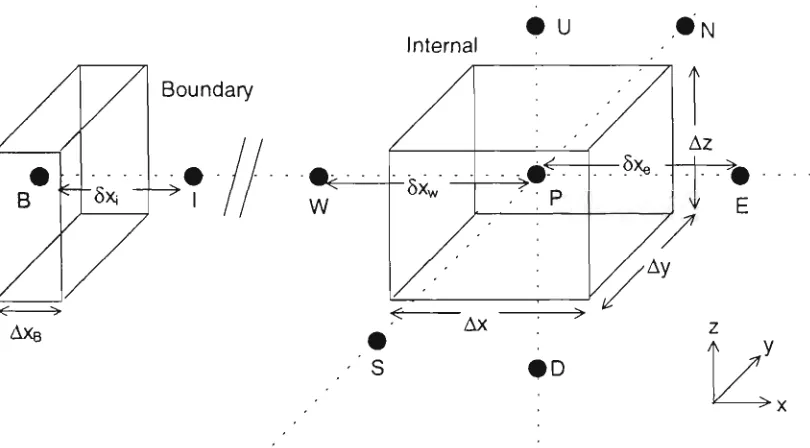
2.3.1. Steady One-Dimensional Heat Conduction 26
2.3.2. Unsteady Heat Conduction 28 2.3.3. Steady Convection and Diffusion 30
2.3.4. Variable Flow Field 32 2.3.5. Iteration and Convergence 37 2.4. THE FIELD MODEL CESARE-CFD 39
2.4.1. Overview 39 2.4.2. Computational Grid 41
2.4.6. Boundary Conditions 50 2.4.6.1. Solid Boundary 50 2.4.6.2. Forced Flow Port 54 2.4.6.3. Balance Port 55 2.4.7. Convergence and Under-Relaxation 57
2.5. CONCLUSION 60
3. ENCLOSURE F I R E MODELLING 61
3.1. INTRODUCTION 61
3.2. THERMAL RADIATION 61
3.3. THEORY OF RADIATIVE HEAT TRANSFER 63
3.3.1. Fundamentals 63 3.3.2. Direct Transfer Between Surfaces 64
3.4. RADIATION FROM AN ABSORBING MEDIUM 66
3.4.1. Absorbing Gases 67 3.4.2. Absorbing Particles 69
3.5. NUMERICAL SOLUTIONS 71
3.5.1. Monte Carlo Method 72 3.5.2. Six-Flux Method 73 3.5.3. The Discrete Transfer Method 74
3.6. RADIATION MODELLING IN CESARE-CFD 76
3.6.1. Particle and Gas Absorption Coefficients 79
3.6.2. Wall Temperatures 81
3.7. EXPERIMENTS 83
3.7.1. Aims 83 3.7.2. Instrumentation and Methodology 84
3.7.3. Results 88
3.8. MODELLING 91
3.8.1. Modelling Method 91 3.8.2. Comparison of Modelling with Experimental Results 94
3.8.3. Comparison of Original and Modified Radiation Models 101
3.9. NUMERICAL INVESTIGATION OF THE MODEL 105
3.9.1. Grid Generation 105 3.9.2. Modelling Results 108 3.9.3. Convergence Analysis 113
3.9.3.4. Medium Grid Unsteady State 123
3.10. SENSITIVITY ANALYSIS 125
3.10.1. Fuel to Soot Conversion 126 3.10.2. Oxygen Limit for Combustion 129 3.10.3. Balance Port Velocity Limit 134 3.10.4. Heat Transfer Coefficient 137 3.10.5. Heat of Combu.stion 140
3.10.6. Summary 143
3.11. PREVIOUS MODELLING WORK 144
3.11.1. A Preliminary Modelling Exercise 144 3.11.2. Comparison of Experimental and Modelled Results 146
3.12. CONCLUSIONS 155
4. COMBUSTION 157
4.1. AIMS 157
4.2. THEORY OF COMBUSTION 158
4.2.1. Thermal Degradation of Solids 158 4.2.2. Thermo-Gravimetric Analysis 159
4.2.3. Ignition 161 4.2.4. Combustion of Solid Fuels 163
4.3. MODELLING OF COMBUSTION 165
4.3.1. Surface Temperature 166 4.3.2. Conduction Within the Solid 168
4.4. COMBUSTION PROPERTIES OF FLEXIBLE POLYURETHANE FOAM 172
4.4.1. Chemistry 173 4.4.2. Physical Properties 173
4.4.3. Thermal Properties 174
4.5. CONE CALORIMETER EXPERIMENTS ON POLYURETHANE FOAMS 175
4.5.1. Aims of the Cone Calorimeter Tests 175
4.5.2. Feasiblity 175 4.5.3. Cone Calorimeter Standard Test Method - ASTM E 1354 177
4.5.4. Experiments 179 4.5.5. Results of Standard Tests 184
5. FLAME SPREAD 208
5.1. INTRODUCTION 208
5.2. PRELIMINARIES 209
5.2.1. The Phenomenon of "Spread" 209
5.2.2. Cellular Automata 210 5.2.3. Modelling with Cellular Automata 216
5.2.4. Further observations on the cellular automata technique 220
5.3. THE PHYSICS OF FLAME SPREAD 221
5.3.1, Fundamentals 221 5.3.2, Opposed Flow Flame Spread 223
5.3.3, Flow Assisted Flame Spread 224
5.3.4, Fire growth 225
5.4. THE FLAME SPREAD MODEL 226
5.4.1, Surface Node Temperatures 227 5.4.2, Configuration Factor of the Flame 228
5.4.3, Internal Nodes 234 5.4.4, Grid Transformation 234 5.4.5, Discretisation of the Heat Equation in the Transformed Co-ordinates 236
5.4.6, Boundary Conditions 239 5.4.7, Solution of the Discretised Equations 241
5.5. STRUCTURE OF THE MODEL 243
5,5,1, Early Modelling Results 246
5.6. FURNITURE CALORIMETER EXPERIMENTS 248
5.6.1, Aims 248 5.6.2, Methods 249 5.6.3, Video Results 250 5.6.4, Experimental Results and Observations 257
5.7. MODELLING RESULTS 260
5.8. SENSITIVITY ANALYSIS 265
5.8.1, Grid Parameters 266 5.8.2. Flame Parameters 272 5.8.3. Material Parameters 276
5.8.4, Summary 281
5.9. CONCLUSION 281
6. FLAME SPREAD IN C F D 283
6.2.1, Solid Fuel Embedding Method 285
6.2.2, Grid Embedding 286 6.2.2.1, Transfer from Solid to Flow 286
6.2.2.2, Transfer from Flow to Solid 288 6.2.3, Convective Heat Tran.sfer at the Gas-Solid Boundary 291
6.2.4, Initialisation of the Model 292
6.3, A SIMPLE TEST CASE 294
6.3.1, Conduction Results 296 6.3.2, Conduction and Convection Results 297
6.3.3, Conduction, Convection and Combustion Results 298
6.3.4, Convergence Analysis 299 6.3.5, Concluding Remarks 301
6.4, EBFF FOAM SLAB EXPERIMENTS AND MODELLING 302
6.4.1, Experiments 302 6.4.2, Modelling 305
6.5, COMPARISON OF EXPERIMENTAL AND MODELLED RESULTS 307
6.6, CONVERGENCE ANALYSIS 324
6.7, FUTURE IMPROVEMENTS ,. 328
6.8, CONCLUSIONS 330
7. CONCLUSIONS 332
7.1, GENERAL CONCLUSION 332
7.2, SPECIFIC CONCLUSIONS 332
7.3, FUTURE WORK 337
REFERENCES 340
APPENDIX A STAND-ALONE FLAME SPREAD MODEL A-1
SPREAD,IN A-1 SPREAD,F A-3 SPREAD,INC A-19
APPENDIX B CFD FLAME SPREAD MODEL B-20
SPREAD,IN B-20 SPREAD.F B-21 SPREAD.INC B-44
APPENDIX C CONFERENCE PAPERS C-45
A Numerical Model for Horizontal Flame Spread over Solid Combustible Fuels C-45
LIST OF FIGURES
Figure 2,1 Control cell in Cartesian co-ordinates 26 Figure 2,2 Control volume for velocity component u 33
Figure 2.3 Automatic filling of grid points 42 Figure 2,4 Flow diagram for CESARE-CFD 47 Figure 3,1 Planck mean absorption coefficient (Tien et al^*^) 80
Figure 3,2 The portion of the Experimental Building-Fire Facility used in this study 84
Figure 3,3 Temperature histories of a few points throughout the test facility 85
Figure 3,4 Carbon dioxide concentration history for Room 103 86 Figure 3,5 Time history of obscuration meter measurements 90 Figure 3.6 The flow grid (a) and radiation grid (b) used in this study 92
Figure 3.7 Predicted and measured heat fluxes to floor level 95 Figure 3,8 Predicted and measured temperatures along the centreline of the bum room 96
Figure 3,9 Predicted and measured temperatures in Room 101 96 Figure 3,10 Predicted and measured COT concentrations in (a) Bumroom (b) Room 101 97
Figure 3,11 Measured versus predicted heat fluxes (kW/m^) 98 Figure 3,12 Measured versus predicted temperatures (°C) 99 Figure 3,13 Comparison of predicted temperatures in Room 101 102
Figure 3,14 Comparison of predicted temperatures in the Bum Room 103 Figure 3,15 Comparison of predicted radiant fluxes to floor level in Bum Room 104
Figure 3,16 Comparison of predicted COT concentrations 104 Figure 3,17 Flow grids (a,b) Coarse (c,d) Medium (e,f) Fine 107 Figure 3,18 Comparison of predicted temperatures in Room 101 109 Figure 3,19 Comparison of predicted temperatures in the Bum Room 109 Figure 3,20 Comparison of predicted radiant fluxes to floor level in Burn Room 110
Figure 3,21 Comparison of predicted COT concentrations 110 Figure 3,22 Predicted carbon dioxide concentration distribution for the three grid refinements 111
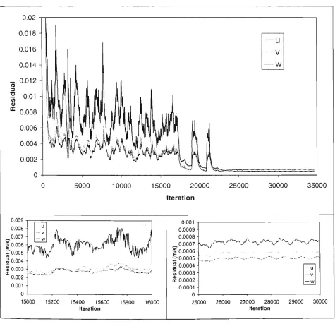
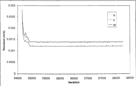
Figure 3,23 Comparison of predicted temperatures for the steady and unsteady solutions 112 Figure 3,24 Velocity residuals for the fine grid 200kW steady state fire simulation 115
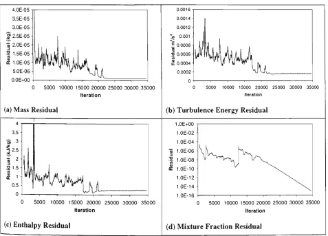
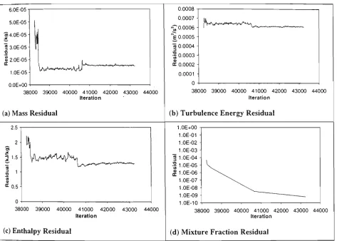
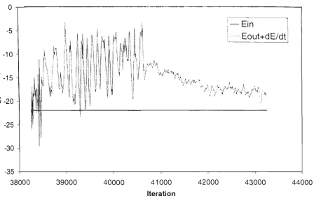
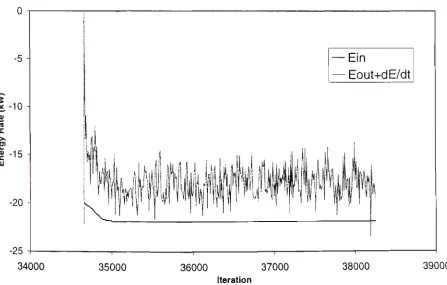
Figure 3,25 Residuals for the fine grid 200kW steady state fire simulation 116 Figure 3,26 Energy balance for the fine grid 200kW steady state fire simulation 117 Figure 3,27 Velocity residuals for the medium grid 200kW steady state fire simulation 118
Figure 3,32 Energy balance for the coarse grid 200kW steady state fire simulation 122 Figure 3,33 Velocity residuals for the medium grid 200kW unsteady state fire simulation 123
Figure 3,34 Residuals for the medium grid 200kW unsteady state fire simulation 124 Figure 3,35 Energy balance for the medium grid 200kW unsteady state fire simulation 124
Figure 3,36 Comparison of predicted temperatures in Room 101 127 Figure 3,37 Comparison of predicted temperatures in the Burn Room 127 Figure 3,38 Comparison of predicted temperatures in Room 103 128 Figure 3,39 Comparison of predicted temperatures in the corridor 128
Figure 3,40 Comparison of predicted CO2 concentrations 129 Figure 3,41 Comparison of predicted temperatures in Room 101 130
Figure 3,42 Comparison of predicted temperatures in the Bum Room 131 Figure 3,43 Comparison of predicted temperatures in Room 103 131 Figure 3,44 Comparison of predicted temperatures in the corridor 132
Figure 3.45 Comparison of predicted CO? concentrations 132 Figure 3,46 Predicted temperature distribution for varying oxygen combustion limit 133
Figure 3,47 Comparison of predicted temperatures in Room 101 135 Figure 3,48 Comparison of predicted temperatures in the Burn Room 135 Figure 3.49 Comparison of predicted temperatures in Room 103 136 Figure 3.50 Comparison of predicted temperatures in the corridor 136
Figure 3,51 Comparison of predicted CO2 concentrations 137 Figure 3,52 Comparison of predicted temperatures in Room 101 138
Figure 3,53 Comparison of predicted temperatures in the Bum Room 138 Figure 3,54 Comparison of predicted temperatures in Room 103 139 Figure 3,55 Comparison of predicted temperatures in the corridor 139
Figure 3,56 Comparison of predicted CO? concentrations 140 Figure 3,57 Comparison of predicted temperatures in Room 101 141
Figure 3,58 Comparison of predicted temperatures in the Burn Room 141 Figure 3,59 Comparison of predicted temperatures in Room 103 142 Figure 3,60 Comparison of predicted temperatures in the corridor 142
Figure 3,61 Comparison of predicted CO2 concentrations 143
Figure 3,62 The flow grid used in original study 145 Figure 3.63 Predicted and measured CO2 concentrations in (a) Bumroom (b) Room 101 147
Figure 3.64 Predicted CO2 concentrations with and without Room 103 148 Figure 3.65 Radiation heat flux to floor level with and without Room 103 148
Figure 3.69 Predicted and measured temperatures in Room 101 152 Figure 3.70 Predicted and measured heat fluxes to floor level 153 Figure 3.71 Predicted and measured CO2 concentrations 154 Figure 4.1 Position of thermocouples for cone calorimeter tests 181
Figure 4.2 Radiation heat flux map 183 Figure 4.3 Rate of heat release of retarded foam at lOkW/m' 185
Figure 4.4 Results of 15 kW/m"cone calorimeter tests on standard foam 187 Figure 4.5 Results of 10 kW/m" cone calorimeter tests on standard foam 188
Figure 4.6 Results of cone calorimeter tests on retarded foam 189 Figure 4.7 Results of 25 kW/m" piloted tests on standard foam 191 Figure 4.8 Results of 35 kW/m^ piloted tests on standard foam 192 Figure 4.9 Results of 35 kW/m" non-piloted tests on standard foam 193 Figure 4.10 Results of 50 kW/m^ non-piloted tests on standard foam 194 Figure 4,11 Results of 50 kW/m^ piloted tests on standard foam 195 Figure 4.12 Results of 70 kW/m^ non-piloted tests on standard foam 196 Figure 4.13 Average effective heat of combustion versus applied heat flux 197
Figure 4.14 Peak rate of heat release versus applied heat flux 198 Figure 4,15 Heat release rate versus applied heat flux at various mass remaining values 199
Figure 4.16 Regression data for the series shown in Figure 4,15 200 Figure 4,17 Temperature measurements for 50kW/m' autoignition test on fire retarded foam, 203
Figure 4,18 Temperature measurements for two lOkW/m' piloted tests on fire retarded foam. 205
Figure 5,1 Moore neighbourhood of a cell 211 Figure 5,2 Spreading configurations for various "minimum neighbour" ignition criteria 212
Figure 5,3 Merging of two burning regions into a single region 213
Figure 5,4 Limiting spread rate configuration 214 Figure 5,5 Geometry of the octagonal spread configuration 214
Figure 5,6 Flowchart for the cellular automata method of flame spread 219
Figure 5,7 Construction of configuration factor 229
Figure 5,8 Node convention 238 Figure 5,9 Flow chart for the stand-alone flame spread model 244
Figure 5,10 Effective flame diameter for half-mattress flame spread test 247
Figure 5,11 Mass loss rate for half-mattress flame spread test 247 Figure 5.12 Video stills of the oscilliating flame 106 seconds after ignition (Test 2) 252
Figure 5,17 Video stills of the spreading flame 90s-165s (Test 3) 256
Figure 5.18 Average mass loss rate for the three tests 258 Figure 5.19 Average rate of heat release for the three tests 258 Figure 5.20 Average effective heat of combu.stion versus time for the three tests 259
Figure 5.21 Average effective heat of combustion versus mass remaining for the three tests... 259
Figure 5.22 Measured and theroretical flame heights 260 Figure 5.23 Predicted and measured flame diameter 262 Figure 5.24 Predicted and measured mass loss rate 264 Figure 5.25 Predicted and measured flame height 264 Figure 5.26 Flame spread and mass loss for varying conduction mode 269
Figure 5.27 Flame spread and mass loss for varying grid size 270 Figure 5.28 Flame spread and mass loss for varying time step 271 Figure 5,29 Flame spread and mass loss for varying flame temperature 273
Figure 5,30 Flame spread and mass loss for varying flame heat factor ^ 274 Figure 5,31 Flame spread and mass loss for varying flame absorption coefficient 275
Figure 5.32 Flame spread and mass loss for varying pre-exponential constant 278
Figure 5.33 Flame spread and mass loss for varying activation energy 279 Figure 5,34 Flame spread and mass loss for varying surface pilot ignition temperature 280
Figure 6,1 Flow cell neighbours 289 Figure 6,2 Linear interpolation method 290
Figure 6,3 The flow grid used in the test cases 295 Figure 6,4 Temperature results of the first and second scenarios 296
Figure 6.5 Temperature results of the third scenario: vertical direction 298 Figure 6,6 Temperature results of the third scenario: horizontal direction 299 Figure 6,7 Velocity residuals for the flame spread test case simulation 300
Figure 6,8 Residuals for the flame spread test case simulation 300 Figure 6,9 Energy balance residuals for the flame spread test case simulation 301
Figure 6,10 The portion of the Experimental Building-Fire Facility used in this study 302
Figure 6,11 Flow grid used in this study 306 Figure 6,12 Effective diameter of flame 309
Figure 6.13 Total mass of fuel slab 309 Figure 6,14 Mass loss rate of fuel 310 Figure 6.15 Time of ignition of cells 313 Figure 6,16 Time of burnout of cells 313 Figure 6.17 Velocity profile at peak burning 314
Figure 6.20 Temperature histories of four key locations 317 Figure 6.21 Species concentration at selected locations 318 Figure 6,22 Mass loss and radiation heat flux histories 318
Figure 6.23 Mass loss rate to heat flux ratio 320 Figure 6.24 Measured (a) and predicted (b) temperatures at the door calorimeter 322
Figure 6.25 Measured (a) and predicted (b) velocities at the door calorimeter 323 Figure 6.26 Measured (a) and predicted (b) oxygen concentrations at the door calorimeter 324
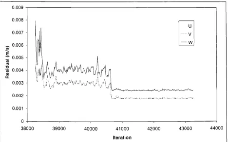
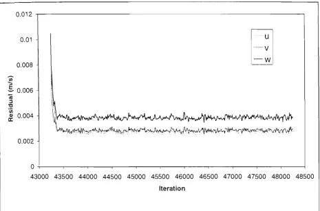
Figure 6.27 Velocity residuals for the full scale unsteady flame spread simulation 325
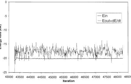
Figure 6.28 Residuals for the full scale unsteady flame spread simulation 326 Figure 6.29 Energy balance residuals for the full scale unsteady flame spread simulation 327
LIST OF TABLES
Table 2,1, Values of exchance coefficients and source terms used in CESARE-CFD 40
Table 3,1 Heat flux measurement 85 Table 3,2 Temperatures (°C) measured in the Bum Room, aty=1.2m 89
Table 3,3 Temperatures (°C) measured in Room 101, atx=l,2m 89 Table 3,4 Temperatures (°C) measured in Room 103, at y=4,2m 89 Table 3,5 Temperatures (°C) measured in the corridor, at y=6,25m 89
Table 3,6 Heat Fluxes (kW/m^) measured at floor level 89 Table 3,7 Carbon dioxide concentrations (kg/kg) measured at various heights 89
Table 3,8, Emissivities of surfaces 93 Table 3,9, Values of constants used in Equation 3,49 93
Table 3,10, Parameters considered in the sensitivity analysis 125
Table 4,1 Kinetic properties of polyurethane foams 161 Table 4,2 Constants required in the combustion and flame spread model 172
Table 4,3, Physical properties of polyurethane foams 174 Table 4,4 Cases tested in the first series of cone calorimeter experiments 180
Table 4,5 Cases tested in the second series of cone calorimeter experiments 180 Table 5,1 Material constants used in the stand-alone flame spread model 261 Table 5,2 Gas phase parameters used in the stand-alone flame spread model 261
NOMENCLATURE
ROMAN
«g
<3k, by, Ck, 4
A, d4, /I,,
A Cm, Lv Cp J D D E E Eb, Eb.x
f
F F 8 h,Ah h H . AH, I i. j . k k k k.KAcceleration due to gravity
Intermediates in Thomas algorithm
Area, area element, bounding surface area
Pre-exponential constant
Mass concentration, volume concentration
Thermal capacity Particle diameter
Characteristic dimension Distance from flame base Activation energy
Wall roughness constant Energy radiated by black body, by black body at wavelength X Fuel mixture fraction
Configuration factor Fraction fuel remaining Fuel fraction fluctuation Enthalpy, change in enthalpy Heat transfer coefficient Flame height
Heat of combustion Intensity
Cartesian indicies
Turbulence kinetic energy Thermal conductivity Extinction coefficient L't L,m Lv m M Mx n n P P AP q
q . Q
r ro R R Rs s S, S^ 5v t T
U, V, w V
V, Vi
x
X, y, z
Yx
Path length, mean beam length Heat of volatilisation
Mass flux Mass
Molar mass of species X Neighbourhood number Refractive index Pressure field Partial pressure Pressure difference Heat Heat flux Radius Fuel/oxygen stoichiometric ratio
Universal gas constant Flame radius
Decomposition rate of solid Distance
Source term of flow variable ^ Surface area per unit volume Time
Temperature
Velocity components Velocity
Volume, flame volume Wall thickness
Cartesian coordinates* Concentration of species X
GREEK
a
a
Pk,5kr,r,
e, Exe,<i)
K KX
^ t Thermal diffusivity AbsorptionIntermediates in Thomas algorithm
Exchange coefficient
Emissivity, emissivity at wavelength A,
Spherical coordinates Absorption constant von Karman's constant Wavelength Turbulence viscosity V
^.^,c
p
a
o<^
X X -e -<t)ea,da
Kinematic viscosity Transformed coordinates Density Stefan-Boltzmann constant Prandtl/Schmidt number of flow variable 0Thermal thickness Transmission fraction Flow variable
Equivalence ratio
Solid angle, increment of solid angle
ABBREVIATIONS AND ACRONYMS ID 3D ADI CESARE CESARE-CFD CFD CSIRO EBBF EHC FDM MIMS PMMA PUF RAM RHR VUT One Dimensional Three Dimensional
Altemating Direction Implicit (method)
Centre for Environmental Safety and Risk Engineering CFD model developed by researchers at CESARE Computational Fluid Dynamics
Commonwealth Scientific and Industrial Research Organisation Experimental Building-Fire Facility
Effective Heat of Combustion Finite Difference Method
Mineral Insulated Metal Sheathed (thermocouple) Polymethylmethacrylate
Polyurethane Foam Risk Assessment Model Rate of Heat Release
CHAPTER l SECTION i.l
1. OVERVIEW
1.1. INTRODUCTION
1.1.1. Fire Safety
Fire may be described as the chemical process by which a fuel reacts in the gaseous phase with an oxidant to produce heat and reaction products. If properly controlled and hamessed, such as in a coal fired power plant or a domestic cooking appliance, this reaction may be greatly beneficial. However, an accidental or uncontrolled fire is often hazardous, and may pose a serious threat to both life and property. The magnitude of the hazard depends on the nature of the fuel, the speed of the reaction, the amount of heat released, the toxicity of the products, the location and situation of the fire, and so forth. A particularly hazardous situation arises when the fire occurs in an enclosure, such as any building stmcture with a ceiling and walls to prevent or restrict the escape of the combustion products. In such an instance, the fire may deplete the enclosure of oxygen, replacing it with toxic combustion products. Conversely, if there is sufficient ventilation to maintain a steady supply of oxygen to the fire, the buildup of hot products close to the ceiling will increase the amount of heat feeding back to the fire source and surroundings. This will cause the fire to grow and in turn heat the combustion products further in a mnaway reaction, a phenomenon called flashover. In a flashover fire, all combustible objects in the vicinity of the original fire become involved in the combustion reaction, and there is a significant release of heat and toxic gases which rapidly spread the fire to other parts of the building or enclosure. Regardless of whether flashover occurs or not, it is the replacement of oxygen with asphyxiating and toxic gases which is responsible for the majority of casualties in building-fires.
CHAPTER 1 SECTION l . I
codes, as often the prescriptive regulations may in some situations be excessive, or lead to levels of redundancy, and therefore add unnecessary costs and restrictions to building design . Development of a performance based code may be accomplished with the aid of an efficient Risk Assessment Model (RAM), which is able to assess the level of protection afforded to occupants and property against a fire, and aims to minimise both the risk, and the cost of providing that protection over the lifetime of the building in question'. Amongst the many components required in a RAM is a comprehensive fire model capable of making accurate predictions of possible fire scenarios in the building or enclosure under consideration, and the time of occurrence of key events within the scenario.
Developing a fire model capable of making the predictions required of a RAM requires a thorough understanding of the physical and chemical processes of fire, in particular those aspects which contribute the most to the overall hazard. Since the RAM needs to be provided with the response times of fire detection and suppression subsystems, and the time available for occupants to make a safe egress before conditions in the building become untenable, the factors relating to fire growth and spread are of particular importance. Babrauskas and Peacock^ have identified four main constituent phenomena comprising a typical' fire growth and spread scenario, namely ignition, flame spread, heat release rate, and the release rate of smoke and toxic gases. While the heat release rate was identified as the most important variable contributing to the fire hazard, the factors are related and all need to be considered in the development of an accurate fire growth and spread model.
1.1.2. Fire Models
The scope of fire modelling goes beyond just providing data for a RAM, which is merely one of many practical applications of fire models. Fire modelling is also a tool for understanding the nature of fire itself; indeed, a model is a mathematical and physical representation of the modeller's understanding of the physical process.
CHAPTER l SECTION i,i
categorises* into empirical, and physical. The main distinction between deterministic models and probabilistic models is that given a .set of initial conditions, only one final result will be forthcoming from a deterministic model, whereas probabilistic models will generally produce a spread of results. This project is concerned with deterministic models, which incorporate the underlying physics of the scenarios they model. The two main types of deterministic enclosure fire models are zone models and field models.
Zone models fall into the "empirical" category of deterministic models. Their initial development precedes the widespread availability of powerful computers, as their relative simplicity allowed the possibility of a solution to the problem in question, which did not require excessive amounts of computation. The models are based on the observation that a flaming fire in an enclosure tends to develop a clear stratification; that is, the smoke and hot gases from the fire rise due to buoyancy to the upper portion of the enclosure, where they spread out forming a layer whose boundary is at a fairly uniform height. At the same time, the cooler "fresh" air remains at the bottom, forming a second distinct layer. Most zone models consist of these two layers, although some also include the fire plume as an additional zone, and possibly one or two other prominent phenomena as extra zones, while some even consider the entire enclosure as a single zone. Whatever the case, the physical properties within each zone are assumed to be constant and homogeneous, and the conservation of energy and mass is observed for each zone, and for the interaction between zones.
The main weakness of zone models is they have been validated against a particular class of enclosure fire, that being mainly domestic style single enclosures. They have not generally been validated for enclosures of a large area, or with large open spaces such as atria, or those possessing complex geometries. Also, they provide limited information about movement of smoke between compartments within an enclosure, as well as many other physical phenomena. However, their relative simplicity means that, running on a typical modem personal computer, they can yield satisfactory solutions to a particular fire problem in a matter of minutes ' ,
CHAPTER 1 SECTION I . l
models. The model is formulated by examining the fundamental physical and physiochemical behaviour of the fire scenario. In fact, due to the plethora of phenomena which contribute to the fire scenario, most field models contain empirical assumptions somewhere in their subroutines, so that in some ways they may be thought of as being just complex zone models. However, these "zone models" contain typically tens of thousands of cells rather than two or three (or a dozen or so if multiple compartments are considered), and can calculate a much wider range of variables, in particular the velocity components of the moving fluids (air and combustion products), and distributions of temperature and heat fluxes. Thus, it is possible to compute in some detail the movement of smoke throughout the enclosure, and the temperature and species distribution within the smoke layer itself. This thesis makes considerable use of CFD modelling: in particular, the model hereafter referred to as CESARE-CFD is widely used, its name derived from having been developed by researchers at the Centre for Environmental Safety and Risk Engineering (CESARE), A more detailed description of this and other models will be given later.
The main drawback of field models is that, in spite of the advances in modern computers, they are still very computationally intensive and require a great deal of time and computer resources to execute. In addition, many of the phenomena they attempt to model are not fully understood; examples include turbulence, chemical reaction kinetics, and the combination of the two, turbulent combustion. Nevertheless, improved computing power and further research into key areas will progressively diminish these problems,
CHAPTER 1 ^ SECTION 1.1
Validation of a field model requires that its predictions be compared with some other quantitative data. For some very simple fire scenarios, this may be in the form of an analytical solution. Zone
models also offer a limited number of data points for comparison, although they themselves require validation. However, a CFD model attempting to make full-scale predictions will, in the majority of cases, require that full-scale experiments be performed for comparison, particularly when complex geometries are involved. Full-scale tests by their nature are more dangerous and more expensive than models, but they are necessary to provide the data needed for validation of the models. Because of their cost, it is necessary that full-scale experiments be well devised, constrained to avoid variable effects, and that the maximum amount of data should be extracted from each experiment.
1.1.3. Flame Spread Modelling
Given that deterministic enclosure fire models have been in use for some time, the question to be asked is, to what extent have they been used to address the factors contributing to fire hazard? Namely, ignition, fire spread, rate of heat release, and rate of product release, as mentioned earlier. Certainly, the rate of heat release is an integral factor of most models, since if there is no heat source, there is no fire, and the modelling becomes a nihilistic exercise. Often, though, this heat "input" into the system is either constant or is specified as a predetermined history. Even for a complex scenario such as the field modelling of the Kings Cross Underground Station fire^, an assumed heat release history was used,* Of course, this need not always be the case, as many models attempt to determine the heat release rate as well as the effect that the heat release has on the enclosure. Heat release may be determined by size of the buming area and hence the combustion rate, which may increase due to flame spread. These models usually take into account the radiant feedback effect that the enclosure has on the combustion rate and rate of spread as well. Typically, the spread rate is an empirical function of the extemally applied heat flux and local oxygen concentration^''. Similarly, empirical relationships are often used for the combustion behaviour, and the release of smoke and other combustion products''.
CHAPTER 1 SECTION 1.2
largely self contained. Even if they employ CFD techniques to calculate the gas pha.se behaviour, the region modelled is in the vicinity of the flame only. If ambient or environmental factors are considered, they are usually assumed, and there is generally no feedback between the buming region and the surroundings. Often these models assume a geometrical configuration, .so that they apply only to upward flame spread, or horizontal radial spread, or some other geometry which reduces the complexity of the problem,
A reason that there is a separation between full-.scale CFD models, used to model the environment associated with fires in full scale enclosures, and detailed flame spread models is possibly one of scale. In modelling a full-scale enclosure using CFD, it is unlikely that grid cells smaller than, say, 50 mm will be used. A typical "standard" room measures 2,4x2,4x3,6 m, so unless a choice is made to discretise the modelled enclosure with literally millions of control cells (a number which is still prohibitively large for all but the most powerful supercomputers), the grid will be necessarily coarse. Of course, that is ignoring the possibility of modelling additional compartments adjoining the room of fire origin. On the other hand, in modelling flame spread, particularly spread in the direction opposite the local fluid flow direction, important phenomena occur at scales of the order of a few millimetres. While future computers may be powerful enough to use a very fine mesh in the vicinity of the buming region, or even for the entire enclosure of interest, for the present it is necessary to develop other techniques to resolve the different scale requirements,
1.2. AIMS OF THE P R O J E C T
1.2.1. General Requirements
The primary aim of the research reported in this thesis is to construct a flame spread model, and then incorporate it in an interactive mode with a CFD model, to accurately predict full-scale fires involving flame spread across solid fuel objects. The flame spread model will be used to predict the contribution of heat and fuel volatiles to the gas phase, whereby the CFD model will be used to calculate the combustion of the fuel and the distribution of heat and products of combustion. At the same time, the CFD model will be used to calculate the heat feedback to the fuel surface within the flame spread model, in turn affecting the flame spread rate and rate of volatilisation of the fuel.
CHAPTER I SECTION 1.2
operate on a di.screte grid, with the properties being uniform over each control cell, as is the case with CFD models. This means that unlike most analytical models of flame spread, the flame front will be characterised as advancing by a series of discrete jumps rather than continuously.
The requirements of the flame spread model as identified previously by the author" are basically threefold. Firstly, in keeping with the spirit of CFD models, the flame spread model must be based as much as possible on first principles. Secondly, it must be geometrically flexible, so that it is capable of modelling a wide variety of flame spread scenarios. These scenarios include horizontal radial spread, horizontal planar, vertical upwards, vertical downwards, and even arbitrary shapes, angles, and orientations. Thirdly, the fundamental material properties required for the model must
17
be experimentally derivable .
In addressing the first requirement, the natural question to ask is: what are the "first principles" involved in flame spread modelling? At a fundamental level, flame spread is an ignition and combustion problem. Evidence of this may be seen in the fact that flame spread properties are closely linked to the heat release rate properties of the fuel in question'"\ This is logical, as preheating of the fuel ahead of the flame front will be in proportion to the amount of heat released from the buming region. It would be expected that as more heat is released, the faster the preheating of the unbumt fuel, and the faster the rate of spread. In light of the discrete namre of numerical modelling, this research will investigate whether the modelling of flame spread may be represented as a series of ignitions of discrete fuel elements, the combustion of which is determined by fundamental material properties.
This approach will help greatly with the geometric flexibility aspect of the second requirement. If the amount of heat received by a fuel element can be determined, it is possible to calculate its ignition and combustion properties, presuming of course that the fundamental material properties are themselves independent of the geometry. However, there are phenomena associated with heat transfer which are significant only close to the flame front. Thus, it will be necessary to develop a method of determining the arrival of a flame front of arbitrary shape. In this research the feasibility of one such technique, developed by the author, based on the methods of cellular automata will be investigated.
CHAPTER 1 SECTION 1,3
and interpreted, can yield fundamental data required for the flame spread model. The data includes the time to, and surface temperature of, ignition as a function of applied radiant heat, heat of volatilisation, chemical kinetics of thermal decomposition, effective heat of combustion of the decomposition products, and so on.
1.2.2. Specific Aims
To summarise, the aims of the project may be expressed as follows
• Identify which submodels encoded in CESARE-CFD, if any, yield inadequate predictions of physical quantities occurring in fire environments, and if possible to rectify these submodels. • Perform appropriate full-scale experiments to acquire data for comparison with model
predictions, and investigate whether changes to the model result in improved predictions.
• Develop an ignition and combustion model that requires fundamental, experimentally derivable material properties. Acquire the required data for a selection of materials by a combination of bench-scale experiments and established literature values,
• Develop a stand-alone flame spread model by combining the ignition and combustion model for an array of fuel cells in conjunction with spread criteria. Use empirical models and assumptions for the gas phase phenomena.
• Perform fumiture calorimeter experiments to investigate the validity of the stand-alone flame spread model,
• Incorporate the flame spread model as a submodel of the field model CESARE-CFD,
• Investigate the validity of the combined CFD-flame spread model by comparing the predicted results with results obtained from a series of realistic full-scale experiments.
1.3. THESIS OVERVIEW
CHAPTER 1 _ ^ SECTION 1.3
The remaining chapters of this thesis reflect the stages which needed to be fulfilled in order to achieve the goal of an integrated CFD model and compatible flame spread model. The first stage, de,scribed in Chapter 3, is to modify the radiation .submodel of CESARE-CFD in order to produce more accurate predictions of radiant heat flux incident at the bounding surfaces of the enclosure (including possible combustible surfaces). As flame spread is sensitive to the heat flux received by the fuel element, and radiation is an important component of this flux, accurate predictions are necessary.
The second stage, described in Chapter 4, deals with the determination of the fundamental combustion properties of solid fuels. While efforts were made to keep the methods general, only two fuels were investigated; namely a standard polyurethane foam and a fire retarded polyurethane foam. These fuels were chosen as they are materials commonly encountered in domestic and commercial occupancies, and have the advantage of being homogenous and isotropic in composition with relatively simple combustion behaviour. They were chosen in favour of materials such as wood which, although one of the most common building materials, is generally non-uniform in composition and directional properties and burns in a complex fashion, and polymethylmethacrylate (PMMA) which, while it has simple uniform combustion properties and has been used extensively in previous combustion and flame spread research'"*''^'^'^, is a somewhat uncommon building and fumishing material.
Chapter 5 deals with the development of a numerical flame spread model, which combines the ignition and combustion methods developed in Chapter 4 with criteria that are used to predict the flame spread. The model was initially developed as a "stand-alone" model, using empirical models for the flame shape and temperature. This is because the cumbersome and time consuming process of encoding, executing, and the inevitable debugging of any model would be further exacerbated by the complexity and lengthy execution time of CFD models.
CHAPTER 2 SECTION 2,1
2. FIELD MODELLING
In this chapter a more detailed description of CFD models is presented, both in general terms, and in particular details are given of the model CESARE-CFD which is the basis of the CFD modelling for the research reported throughout this thesis. The aim of this chapter is to establish the methods involved in constructing a CFD model, and how these methods are incorporated within CESARE-CFD. A description of some of the boundary conditions and convergence criteria which apply to the modelling work throughout the thesis are also included, A review is also presented here, to identify similar modelling work which appears in the literature.
2.1. REVIEW
Although the fundamental equations describing fluid flow have been established for over a century, field modelling became a prominent fire modelling tool around twenty years ago, when computer technology had advanced to the point at which it became feasible to numerically calculate the equations which govem the behaviour of fires. The development of numerical methods suited to computation occurred in tandem with the development of computing power, as the methods became feasible, and could be tested. There was considerable research by workers such as Launder and Spalding (see reference 18 for example) in improving the computational accuracy of mrbulence calculations, and by Patankar and others in developing methods for numerically solving the coupling between pressure and velocity fields, Patankar's classic secondary text'^, first published in 1980, describes the methods, particularly the finite volume techniques, which form the basis of many field models today. It was only another year or two before fire field models were regularly being used and validated^",
CHAPTER 2 . ^ SECTION 2,1
a single commercial package stretch the resources of many institutions, and indeed concern has been rai.sed about the availability of such models for the purpo.ses comparative .scratiny~\ Comparisons showed that both models overall made good predictions of the flow in a simple compartment fire, but that discrepancies occurred close to the boundaries of the enclosure, possibly as a result of the different formulations of the boundary conditions in the models.
The use of CFD models for modelling combustion and fire scenarios comprises only a portion of the overall field of applications for such models. Fluid dynamics encompasses a broad range of topics, including classic problems such as air flowing over an aircraft wing or water flow through a pipe. Combustion modelling is a particular class of fluid flow problem, the difficulty of which is compounded by the fact that the fluid being modelled is undergoing a change of composition and specific volume as it flows. Furthermore, heat transfer to and from the fluid is an important component of modelling combustion processes, CFD combustion modelling itself covers a broad range of subjects, with CFD models finding applications such as modelling the gasification of biomass^"* or coal^"\ the operation of incinerators^^ and fumaces'^, or small scale phenomena such as the combustion of wood samples in a cone calorimeter'^**. Of interest in this thesis, though, is the enclosure fire, which as the name suggests is a fire which takes place in a confined region, with a limited number of openings (or possibly none) to the surroundings.
What is the role of field models in the modelling of enclosure fires? Much has been written about both the merits and shortcomings of zone and field models"'"'*'^, although the usual consensus is that there is, and probably always will be, a need and a use for both. The role of the field model is to provide the detail which the zone model cannot, which in some cases may even provide insights into the nature of the fire itself, A good illustration of this is demonstrated in the modelling of the King's Cross Underground fire^. Field modelling was undertaken to determine if there were any aerodynamic effects which may have contributed to the rapid spread of the fire. This modelling led to the discovery of the so called "trench effect", whereby a flame in an inclined trench such as an escalator will tend to "adhere" to the floor of the trench. This effect was later verified experimentally.
CHAPTER 2 SECTION 2,1
modelling should not be accepted in blind faith. All modelling must be held up to scmtiny, and the cycle of model prediction and experimental verification, or experimental contradiction and model readjustment will inevitably continue, as it does with any scientific process.
It is perhaps the vision of present-day modellers that there will ultimately be a model capable of accurate, detailed, and comprehensive predictions of any arbitrary fire scenario; a "perfect" model. Such a model, as well as providing a detailed description of fluid phase phenomena, such as the concentration and composition of the products of combustion and their movement throughout the enclosure, would also include a physical description of the fuel, including the combustion behaviour of its constituent components. Also included would be the ignition characteristics, growth and spread behaviour of the flame, as well as the heat feedback from the products back to the buming fuel, and even the interaction of the fire environment with fire suppression systems such as sprinklers. Indeed, in a comprehensive model, the presence of walls or a ceiling would be optional, making them just as applicable to open fires as enclosure fires. Such a model does not yet exist', and research continues in attempting to bring it about (including the development of the computing power required for its execution).
Most work currently undertaken in enclosure fire models does not attempt to include all the phenomena required in the "perfect" model, as many aspects are still unknown or untested. Rather, attention is normally focused in a particular study on one or a few aspects at a time. Since enclosure geometry is a variable factor, many modelling exercises, and the experiments undertaken to validate the models, are performed with a simple geometry, usually a rectangular enclosure' " " " , and often with a door placed centrally in one wall, creating a plane of symmetry" , The simplicity of the geometry makes independent experimental reproducability more likely, and therefore more open to scmtiny and critical assessment. The simplicity of the geometry also minimises the effects of the geometry itself, so that other phenomena can be investigated in a controlled fashion.
CHAPTER 2 SECTION 2,1
approaches produced similar temperature distributions, inclusion of the combustion model produced a more realistic flow profile through the compartment opening. This is to be expected, as the flow pattern depends on the volume change associated with the chemical reaction. It does highlight, however, that if ventilation flow rates are important to the application of the fire model, then combustion should be considered. Both modelling exercises by Chow were compared with data produced by Steckler et al", although it was noted that there were insufficient data acquired in the test to provide confidence in the validation of the model. Other issues raised included whether the absence of an adequate radiation model might also be a source of discrepancies.
The effect of thermal radiation on the flow field in a fire has been investigated by Kumar et al"'' for a simple rectangular enclosure. The study likewise used the flow data of Steckler et af", and investigated the effect the presence or absence of a radiation model has on the predictions of the flow rate. As might be expected, the inclusion of a radiation model improved the modelled predictions. The reason that it should be expected is the nature of thermal radiation. The radiant heat output of a hot body is proportional to the fourth power of the absolute temperature, so that radiant heat temperature becomes increasingly dominant as temperature increases, A fire plume is typically at a very high temperature (around 1000°C or higher), which renders radiation heat transfer a significant component of total heat transfer within the enclosure containing the fire plume. Lewis et al"^^ also investigated the effect the inclusion of a radiation model has on the computed upper layer temperature in a compartment, also making comparisons with the experimental data of Steckler et al"^^. It was found that the inclusion of a radiation model improved the prediction of the flow temperatures in the upper region of the enclosure. The importance of accurate radiation heat transfer modelling has been touched upon here. As it forms a significant portion of the work presented in this thesis, a more detailed investigation of radiation heat transfer, and its role in CFD modelling, is left for Chapter 3,
CHAPTER 2 , SECTION 2.1
borne out in the work of Lewis et al^^ who found that the inclusion of a radiation model improved the layer definition. Other mechanisms proposed by Kerrison et al for the layer smearing were inadequacies in the turbulence model, or false diffusion due to the upwind discretisation scheme^^. The upwind scheme is a numerical mechanism employed to reduce numerical instability in flows
which are strongly one-directional, and is described in detail by Isenberg and de Vahl Davis". While it is unconditionally stable (i,e, the method will converge, regardless of the grid size and time step cho.sen), it does lead to a diffusion-like term ("false diffusion") which could feasibly produce the discrepancies observed by Kerrison et al. This effect is noted here, as it will be encountered again later in this thesis.
Another relatively simple geometry which has been investigated is the flow generated by a pool fire in a large wind tunnel"'^'''^. Full scale experimental and modelling tests were undertaken to provide an understanding of the behaviour of fires in elongated enclosures, such as a ventilated mine roadway, or vehicular tunnel. The study yielded useful information regarding the flow rates required to prevent the buoyant backflow of products, as well as providing further validation opportunity for the code. The findings emphasise the importance of accurate radiation modelling of the smoke products, and of the critical role of buoyancy terms in k-e turbulence equations, in successfully predicting the backflow phenomenon. This has similar implications for any model which attempts to make predictions of smoke spread in ventilated enclosures.
While simplified geometry is useful for validation exercises, the geometry of practical applications is often quite complex. Geometry is an important aspect of a fire scenario, and field modelling of more realistic enclosure geometries is undertaken both as further validation exercises of field models"\ and as a practical exercise in determining fire safety of a given enclosure. Whilst experimental data for complex geometries are useful, and efforts to continue their acquisition should be made, modelling exercises are not, and should not, be limited to cases for which experimental data are available. Validation for simple geometries should attribute confidence in a model's ability to make at least qualitative predictions of more complex geometries. For instance, Hadjisophocleous and Cacambouras^' again use the data of Steckler et al,'*'' to validate their code, then with the confidence of validation, explore the effect of several factors including opening size, location of the fire within the enclosure, and the presence of large internal objects in the enclosure. The predictions thus issue a challenge to the experimentalist for verification.
CHAPTER 2 . SECTION 2,1
con.struction of the grid is otherwise straightforward. The flow equations in the model are typically discretised using a finite difference method**", and take their simplest form in such co-ordinates, so that computational effort is minimised. On the other hand, enclosures which include walls not meeting at right angles, or that have curved .surfaces, are more difficult to model. If a rectilinear grid is established for the finite difference method, then such surfaces will manifest themselves as step-like boundaries of the flow region. One remedy is to mathematically transform the non-rectilinear space into one that is non-rectilinear. The transformation results in additional terms appearing in the discretised equations. Another remedy is to fit the grid to the geometry, and to apply the finite element method to derive the governing equations of the flow. However, the equations are in a more complex form than for finite difference, so are computationally more demanding to solve, Ravichandran and Gouldin"^ performed a comparison of finite element and finite difference methods for an incinerator of complex shape. It was found that the finite element method produced more accurate results, and the solution showed less variation with mesh refinement, than the finite difference. However, the method was far more computationally intensive, especially when full combustion and turbulence was considered in the equations.
One of the greatest challenges still facing the development of field models is their so-called "validation", Kerrison et al " describe "validation" (with quotation marks) as the systematic comparison of predictions with experimental results. Hence, a model is presumably deemed to be "valid" if the comparisons are favourable. However, comparison is by no means a trivial exercise, as field models make predictions about thousands (even millions) of data points, whereas only a limited number of data points can be measured in an experiment (perhaps a thousand in an extensively instmmented steady state experiment where measuring devices are movable, and one or two hundred in unsteady fires where devices are likely to be fixed). Since comparison at every point is not feasible, agreement is usually sought at key locations, such as the centreline of the room of fire origin, or profiles of variables across the enclosure opening. If agreement between model and experiment is good at these key locations, then some confidence may be expressed about the modelling results at other locations.
CHAPTER 2 SECTION 2,2
commercial fire field model such as JASMINE or FL0W3D for comparison, although such work is beyond the .scope of this thesis,
2.2. COMPONENTS OF FIELD MODELLING
This section outlines the methodology used to formulate a fire field model. The description begins with the conservation equations which govem heat, mass and momentum transfer within a fluid. Following this is a description of additional components of a field model which are required for fire modelling applications, such as turbulence models and combustion models. Finally, a description is given of the numerical methods required to solve the basic conservation equations.
2.2.1. Conservation Equations
At the heart of field models lie the general conservation equations, the prototypal form of which is
^ + V.pa(|) = V - r 3 + S, (2.1)
where p is the fluid density, u is the local fluid velocity, and ^{x,y,z,t) is the quantity which is being conserved. This quantity may be fluid momentum, temperature, concentration of a chemical species, or turbulence kinetic energy, amongst other properties, and in its general form is a function in three dimensions with time dependence.
CHAPT>:R 2 SECTION 2.2
function of 0 it.self, or it may have spatial and temporal dependencies. If it is a constant, the third term may be rewritten
vr,V(t) = r , v > (2.2)
The source or sink term, S$, corresponds to the amount of the quantity being produced or removed in situ, rather than being transported into or away from the point in question. Such terms may arise, for instance, with thermal energy conservation, where radiant heat is being absorbed or emitted, or in a species mass conservation equation when a particular chemical species is being produced or consumed by a chemical reaction.
In the special case when (j) is the local momentum of the fluid. Equation 2.1 is known as the Navier-Stokes equation, developed over 150 years ago'*. The Navier-Navier-Stokes equation may be expressed in suffix notation by the equation
3M: du- dp 3^/, 1 ^^jj
p—!--l-pM-—'- = — + —^ + ^ (2.3)
dt dXj dx- dx I 3 3x,
where p is the pressure, and r^ is the viscous stress tensor, given by
f,y = 2[is:j (2.4)
where |J. is the molecular viscosity, and sij is the strain-rate tensor, given by
1
^-1- - (2.5)
There are four unknown quantities appearing in the Navier-Stokes equation, namely the three velocity components and pressure. However, there are only three equations in Equation 2.3, one for each value of /, so there are only three equations for four unknowns. An additional equation is required, namely the continuity equation, given by
| ^ + V-(p«) = 0 (2.6)
at
If the flow is incompressible, the density is constant, and Equation 2,6 simplifies to
CHAPTER 2 SECTION 2,2
2.2.2. Turbulence
Solving Equation 2.1 is reasonably straightforward when the velocity is laminar throughout the control volume. However, in many flow problems, such as those involving extensive buoyancy driven flows which occur in building-fires, turbulent flow is almost always present. Turbulent flow
is disorderly and chaotic in nature, with the fluid flowing in a dynamic, ever-changing pattern of whoris and eddies, which are present on scales down to a microscopic level at which the viscosity of the fluid dominates the smallest eddies , With the current computer technology, CFD models cannot resolve down to this small scale, especially when dealing with generic full-scale building-fires.
The random nature of turbulence may be dealt with in a statistical manner, using the methods first developed by Reynolds in 1895, The velocity (hence its momentum) of a fluid flowing turbulently at a given point may be divided into two components; the mean velocity, and the variation about the mean, due to the random fluctuations in velocity resulting from the turbulence. This is expressed in the following notation
u. = (/, + «; (2.8)
where M, is the instantaneous velocity, (/, is the time-averaged velocity, and w' the fluctuating velocity. The corresponding fluctuations in pressure, p, can be expressed in a similar fashion. Since it is the time-averaged conditions which are of concern in fluid modelling. Equation 2,8 is substituted into the Navier-Stokes equation (Equation 2,3), and the time average is taken, to yield the Reynolds-averaged Navier-Stokes equation. This is best illustrated for incompressible fluids. In this case, the Reynolds-averaged Navier-Stokes equation is given by
p - - ^ + pC/^—^-^pw —^ = - - - + - ^ (2.9)
at dx I dXj dXj dXj
CHAPTER 2 SECTION 2,2
The last term is known as the Reynolds stress tensor, denoted t,,. As it is symmetric, there are 6 independent terms, all of which are unknown. These unknowns are in addition to the four time averaged unknowns, without any increa.se in the number of equations; in other words, there are now more unknowns than equations. The system of equations is said to be unclosed.
In order to close the system of equations, it is necessary to make some approximations for the unknown quantifies, based on known flow properties. Some of these approximations have an empirical basis, while others are based principally on a dimensional argument. The first step in this procedure is to introduce the quantity k, the turbulence kinetic energy, defined by
k = —U:U: = _1_
2p ^ii (2.11)
Algebraic manipulation of products of fluctuating quantities with the Reynolds-averaged equation yield the following transport equation for the turbulence kinetic energy 42
dk ^, dk _ ^ dU:
dX: '^ dX; pe + dX: dk
| X - -pM,.«,.M. - p Uj
dX: 2
(2.12)
where e is the rate of dissipation of turbulence kinetic energy per unit mass, defined by
e = V-I ! I_ du' du'
dx^ dx^
(2.13)
However, there are still several unknowns in Equation 2,12, although there are physical interpretations which can be attributed to these terms. It is a common practice to assume that the Boussinesq approximation holds for the Reynolds stress tensor*', i,e.
x,j=2ii^S.j-~pk6.^ (2.14)
where [ij is the eddy viscosity, A further approximation is made for the last two terms in the brackets of Equation 2,12, namely that the sum of the two terms behaves as a gradient-transport process"* , described by
• l - T - T T ^ — T T Mr ^k p Uj
a^ dxj
(2.15)
where a* is the Prandtl number for turbulence, which in most instances is chosen to be a constant. With these approximations. Equation 2.12 can be written in the form
dk ,, dk 9(7, a
^ 1 + ^ ait O* )^x^
CHAPTER 2 . SECTION 2,2
This turbulence transport equation is common to many closure methods. There are two remaining unknowns in the system of equations which need to be accounted for to complete closure. They are the dissipation, e and turbulence length scale, /, Dimensional arguments suggest that the.se terms are related to turbulence kinetic energy by
e oc — (2.17)
One equation models are so called because they use only the turbulence transport equation. Closure is completed by taking Equation 2,17 and mulfiplying the right hand side by a constant of proportionality, which is another closure coefficient. The remaining unknown in the turbulence transport equation, turbulence length scale, must be specified by some means. This usually requires some knowledge of the behaviour of the turbulence in the problem of interest.
Two equation models, on the other hand, introduce a second equation which calculates either the mrbulence length scale, or an equivalent. The most commonly used of the two-equation models is the k-z model. In this model, an equation for the transport of dissipation, e, is derived by a similar methodology to the turbulence transport equation. In doing so, a plethora of additional terms is generated, for which further closure approximations must be made ', In summary, the transport equation for the dissipation rate is given by
ae ,, ae ^ 8 dU: _ £- a
P3: + P ^ ; 3 r = ^^'T^.:/37'-^e2P^ + ' \^r^
ae
ax,
(2.18)dt " ^ dx.^ ' ' k " dXj '"^ k dXj
and the eddy viscosity given by
|I^ = p C — (2.19)
^ e
where Gg, Cei, €^2, and C^u are closure coefficients.