Tight Proofs of Space and Replication
Ben Fisch
Abstract
We construct a concretely practical proof-of-space (PoS) with arbitrarily tight security based on stacked depth robust graphs and constant-degree expander graphs. Aproof-of-space (PoS) is an interactive proof system where a prover demonstrates that it is persistently using space to store information. A PoS is arbitrarily tight if the honest prover uses exactly N space and for any > 0 the construction can be tuned such that no adversary can pass verification using less than (1−)N space. Most notably, the degree of the graphs in our construction are independent of, and the number of layers is onlyO(log(1/)). The proof size isO(d/). The degree ddepends on the depth robust graphs, which are only required to maintain Ω(N) depth in subgraphs on 80% of the nodes. Our tight PoS is also secure against parallel attacks.
Tight proofs of space are necessary for proof-of-replication (PoRep), which is a publicly verifiable proof that the prover is dedicating unique resources to storing one or more retriev-able replicas of a file. Our main PoS construction can be used as a PoRep, but data extraction is as inefficient as replica generation. We present a second variant of our construction called
ZigZag PoRepthat has fast/parallelizable data extraction compared to replica generation and maintains the same space tightness while only increasing the number of levels by roughly a factor two.
1
Introduction
Proof-of-space (PoS) has been proposed as an alternative to proof-of-work (PoW) for applications such as SPAM prevention, DOS attacks, and Sybil resistance in blockchain-based consensus mechanisms [18, 21, 31]. Several industry projects1 are underway to deploy cryptocurrencies similar to Bitcoin that use proof-of-space instead of proof-of-work. Proof-of-space is promoted as more egalitarian and eco-friendly that proof-of-work because it is ASIC-resistant and does not consume its resource (space instead of energy), but rather reuses it.
A PoS is an interactive protocol between a prover and verifier in which the prover use a minimum specified amount of space in order to pass verification. The protocol must have compact communication relative to the prover’s space requirements and efficient verification. A PoS is persistent if repeated audits force the prover to utilize this space over a period of time. More precisely, there is an “offline” phase in which the prover obtains challenges from a verifier (or simulates them non-interactively via Fiat-Shamir), generates an advice stringSthat it stores, and outputs a compact tagτ to the verifier. This is followed by an “online” challenge-response protocol in which the prover uses its advice S to efficiently compute responses to the verifier’s challenges. The soundness of the PoS relies on timing bounds on the online prover’s runtime enforced by frequent verifier audits. Timing bounds are necessary as otherwise the prover could
store its compact transcript and simulate the setup to re-derive the advice whenever it needs to pass an online proof. If the PoS resists parallelization attacks then it is unconditionally secure in this audit model because the prover must use the minimum amount of space to pass challenges within the wall-clock time allotted. Alternatively, soundness is reasoned through a cost benefit analysis; it is assumed that arational prover will not trade significant computation for a relatively small reduction in its space utilization.
In an (S, T)-sound PoS protocol where the prover commits to persistently utilizeN blocks of space, the honest prover uses S =O(N) persistent space and any adversary who passes audits in less than timeT provably usesS = Ω(N) space. There is generally a gap between the honest space utilization and the lower bound on the adversary’s space. If the honest prover uses N
space and some adversary might be able to use N space then this PoS has an space gap. A
tight PoS makes arbitrarily small depending on a construction parameter that will typically impact concrete efficiency. All else equal, a tighter PoS is obviously more desirable as it has tighter provable security. Nearly all existing PoS constructions have enormous space gaps [2,18], including those that are currently being used in practice. The one exception is a recent PoS protocol by Pietrzak [33] based on depth robust graphs, although it does not achieve a tight space gap for concretely practical parameters.
Proof-of-replication (PoRep) [1, 19, 20, 33] is a recently proposed hybrid of PoS with proof-of-retrievability (PoR) [23]. A PoR demonstrates that the prover can retrieve a particular data file of interest, either known to the verifier, committed in a public commitment, or privately preprocessed by a client who produces a verification tag for the file. A PoRep demonstrates that the prover is dedicating unique resources to storing a retrievable copy of the file, and is therefore auseful proof of space. It has therefore been proposed as an alternative Sybil resistance mechanism that is not only ASIC resistant and eco-friendly, but also has a useful side-effect: it provides file storage on real data. Furthermore, since the prover may run several independent PoReps for the same file that each require unique resources, PoReps may be used as a publicly verifiable proof of data replication/duplication.
A PoRep is required to be a PoS, and its security as a proof of data replication is closely related to the space gap of the PoS. Formally, the security notion for PoReps is -rational replication [19], which says that an adversary can save at most an fraction of its space by deviating from storing the data in a replicated format. Storing data in a replicated format is therefore an -Nash-equilibrium. This is the best possible security notion because a prover can always sabotage its replicated format by scrambling its storage in an efficiently decodable (yet no longer replicated) way. A PoRep that satisfies -rational replication is also a PoS with an space gap. Intuitively, if a PoRep is not a tight proof of space then there may be some adversary that would be rationally incentivized to deviate from honest behavior and therefore likely destroy the replication format. This gives a whole new relevance to tight proofs of space, because the security of PoReps is only meaningful when is reasonably small.
The goal of this work is to construct a practical and provably tight PoS that can also be used as PoRep that satisfies -rational replication for arbitrarily small.
1.1 Related work
labeling of the graph using a collision-resistant hash function where the label ev on each node v ∈ G of the graph is the output of the hash function on the labels of all parent nodes of v. It outputs a commitment to this labeling along with a proof (either interactive or non-interactive) that the committed labeling was “mostly” correct. This offline proof consists of randomly sampled labels and their parent labels, which the verifier checks for consistency. During the online challenge-response phase the verifier simply asks for random labels that the prover must produce along with a standard proof that these labels are consistent with the commitment. Their construction leaves a space gap of at least 1− 1
512.
The construction of Ren and Devadas from stacked bipartite expander graphs dramatically improved on the space gap, although it is not secure against parallel attacks. Their construction involves λlevels V1, ..., Vλ consisting of nnodes each, with edges between the layers defined by
the edges of a constant-degree bipartite expander. The prover computes a labeling of the graph just as in the Dziembowski et. al. PoS, however it only stores the labels on the final level. Otherwise, the protocol is roughly the same. Their construction still leaves a space gap of at least 1/2 (and much larger with practical parameters, e.g. their construction requires at least degree 40 graphs to achieve a space gap of less than 2/3).
Recently, Abusalah et. al. [2] revived the simple PoS approach based on storing tables of random functions. The basic idea is for the prover to compute and store the function table of a random function f : [N] → [N] where f is chosen by the verifier or a random public challenge. During the online challenge-response the verifier simply asks the prover to invert f
on a randomly sampled point x ∈ [n]. The intuition for why this should be secure is that a prover who has not stored most of the function table will likely have to brute force f−1(x), performing Ω(N) work. Unfortunately, this simple approach fails to be a PoS due to Hellman’s time/space tradeoffs which enable a prover to succeed with S space andT computation for any
ST =O(N). However, Abusalah et. al. build on this approach to achieve a provable time/space tradeoff ofSkT = Ω(kTk). This PoS is not secure against parallel attacks, and also has a very large (even asymptotic) space gap of 1−64 log1 N.
Pietrzak [33] and Fisch et. al [20] independently proposed a simpler variant of the graph labeling PoS by Dziembowski et. al. based solely on pebbling a depth robust graph (DRG). A degree d DAG on n nodes is (α, β)-depth robust if any subgraph on αn nodes contains a path of at least length βn. It is trivial to construct DRGs of large degree (a complete DAG is depth robust), but much harder to construct DRGs with small (constant or poly-logarithmic) degree. Achieving constant α, β is only possible asymptotically with degree Ω(logN). Simply instantiating the graph labeling PoS on a DRG results in a PoS with a 1−α space gap that is also secure against parallel attacks. Fisch et. al. also suggested combining this labeling PoS with averifiable delay function (VDF) [11] to increase the expense of labeling the graph without increasing the proof verification complexity. The delay on the VDF can be tuned depending on the value of n. Both of these constructions were proposed in the context of designing PoReps. In this variant of the PoS protocol, the prover uses the labeling of the graph to encode a data file onnblocksD=d1, ..., dn. Theith labelei is computed by first deriving a keyki by hashing the labels on the parents of the ith node, and then setting ei = ki⊕di. If all the labels are
stored then any data block can be quickly extracted from ei by recomputing ki. We’ll call this
a DAG encoding of the data input. The VDF approach uses an additional encoding scheme (enc,dec) inside the DAG encoding, where enc is sequentially slow and dec is fast, to derive
ei=enc(ki⊕di). The data is decoded by computingdi =dec(ei⊕ki).
the time bound βn on the prover’s required computation to defeat the PoS. Moreover, while there exist constructions of (α, β) DRGs for arbitrarily small α, these constructions are purely theoretical and are not viable in practice. Pietrzak [33] improved on the basic construction by relying on a stronger property of special DRGs [6, 32] that are (α, β, O(logn/))-depth robust for all (α, β) such that 1−α+β ≥1−. In Pietrzak’s modified construction, the prover builds a DRG on 4n nodes and only stores the labels on the topologically last n nodes. This can similarly be used as a PoRep where the data is encoded only on the last level and the labels on previous levels are just used as keys. This sacrifices on data extraction time because extracting the data requires recomputing most of the keys from scratch, which is as expensive as the PoS initialization.
Pietrzak shows that a prover who deletes an 0 fraction of the labels on the last n nodes will not be able to re-derive them in fewer than n sequential steps. The value 0 can be made arbitrarily small, but at the expense of increasing the degree of the graph proportionally to 1/0. Moreover, although these special DRGs achieve asymptotic efficiency and are incredibly intriguing from a theoretical perspective, they still do not have concretely practical degree. According to the analysis in [6], achieving just a 1/2 space gap with a PoS on N 32 byte data blocks in Pietrzak’s construction would require instantiating these graphs with degree 2,760 logN. The proof size is at least O(λd), so even for λ = 10 (i.e. 10 bit security) and
N = 230 the proof size would be at least 26MB. Furthermore, as decreases λ = O(1/) to maintain the same security level. To achieve a space gap of 1/10 with 10-bit security would required= 19,310 logN andλ= 60 for a proof size of at least 1GB.
Boneh et. al. [11] describe a simple PoRep (also a PoS) just based on storing the output of a decodable VDF on N randomly sampled points, which generalizes an earlier proposal by Sergio Demian Lerner [25]. This is in fact an arbitrarily tight PoS with very practical proof sizes (essentially optimal). However, the time complexity of initializing the prover’s O(N) storage is O(N2), and therefore is not practically feasible for large N. This construction is similar to the PoS based on storing function tables [2], but uses the VDF as a moderately hard (non-parallelizable) function on a much larger domain (exponential in the security parameter) and stores a random subset of its function table. The reason for the large initialization complexity is that the prover cannot amortize its cost of evaluating the VDF on the entire subset of points. In an independent concurrent work, Cecchetti et. al [14] developed a similar idea to our stacked DRGs, using butterfly networks instead of expander graphs, to construct a primitive they called publicly incompressible encodings (PIEs). We elaborate on a comparison in the Appendix.
1.2 Summary of Contributions
We construct a new tight PoS based on graph labeling with asymptotic proof size O(logN/) where is the achieved space gap. We can instantiate this construction with relatively weak depth robust graphs that do not require any special properties other than retaining Ω(N) depth in subgraphs on some constant fraction of the nodes bounded away from 1 (e.g. our concrete analysis is for 80% subgraphs).
to this graph construction asStacked DRGs. We are able to show that this results in a PoS that has only anspace gap. Intuitively, the expander edges between layers amplify the dependence of nodes on the last layer and nodes on earlier layers so that deletion of a smallfraction of node labels on the last level will require re-derivation of nearly all the node labels on the first several layers. Thus, since every layer is a DRG, recomputing the missing fraction of labels requires Ω(N) sequential computation. It is easy to see that this would be the case if the prover were only storing (1−)nlabels on the last level and none of the labels on earlier levels, however the analysis becomes much more difficult when the prover is allowed to store any arbitrary (1−)n
labels. This analysis is the main technical contribution of this work. Concretely, we analyze the construction with an (n,0.80n,Ω(n)) DRG, i.e. deletion of 20% of nodes leaves a high depth graph on the 80% remaining nodes, regardless of the value of.
Our construction is efficient compared to prior constructions of tight PoS primarily because we can keep the degree of the graphs fixed for arbitrary while only increasing the number of levelslogarithmicallyin 1/. In a graph labeling PoS, the offline PoS proofs sampleO(1/) labels along with their parent labels, which the verifier checks for consistency. Thus, any construction based on this approach that requires scaling the degree of graphs by 1/also scales the proof size by 1/, resulting in a proof complexity of at leastO(1/2). In our stacked DRG PoS construction the offline proof must include queries from each level to prove that each level of computed labels are “mostly” correct. If done naively, O(1/) challenge labels are sampled from each level, resulting in a proof complexity O(d/·log(1/)) wheredis the degree of the level graphs. This is already an improvement, however with a more delicate analysis we are able to go even further and show that the total number of queries over all layers can be kept at O(1/), achieving an overall proof complexityO(d/).2
The PoS onStacked DRGs can also be used as the basis for a PoRep that satisfies-rational replication for arbitrarily small .
The PoRep variant on this PoS simply uses the labels on the `−1st level as keys to encode the n-block data input D =d1, ..., dn on the `th (last) level, using the same method described earlier for encoding data into the labels of a PoS (see Related Work, [19, 20, 33]). However, extracting data from this PoRep is as expensive as initializing the PoRep space because it requires recomputing the keys on the`−1st level.
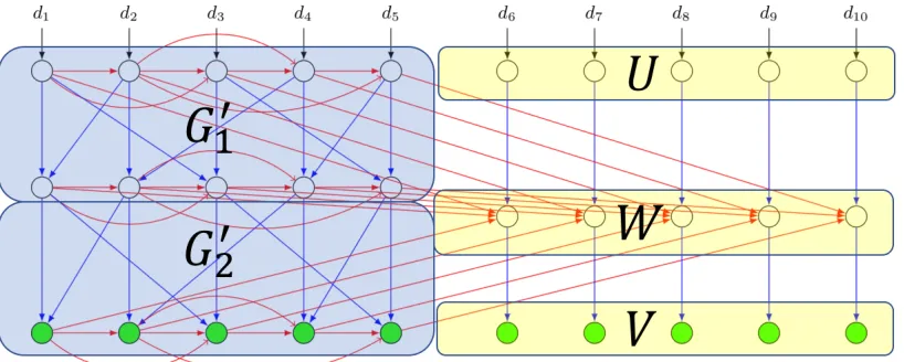
PoRep from ZigZag Expander DRGs Our second contribution is a variant of the PoS on Stacked DRGsthat compromises slightly on efficiency (requires double the number of levels for the same security guarantee) but improves the efficiency of extracting data when this is used as a PoRep. Instead of adding edge dependencies between the layers, every layer is the union of a DRG and a constant degree non-bipartite expander graph. The only edges between layers are between nodes at the same indices. Since the graph is a DAG this means that the union of a subset with its dependencies and targets is a constant fraction larger than the subset itself. By alternating the direction of the edges between layers, forming a “zig-zag”, the dependencies of a subset in one layer become targets of the same subset in the adjacent layer, and the dependencies between layers expands. We refer to this graph construction as ZigZag DRGs. The PoRep on ZigZag DRGs encodes in the labels of each layer the labels of the previous levels. The edges within a layer enforce dependencies between labels by deriving a key for each encoding using a
2
cryptographic hash function. A special key is derived for the encoding on eachith node from the labels on the parents of theith node within the same layer. Essentially, this construction iterates the basic DAG encoding of the data inputs`times (treating each layer as an independent DAG) rather than performing a long key derivation. The labels in any layer can be used to recover the labels in the preceding layer. Furthermore, the decoding step can be done in parallel.
c1 c2 c3 c4 c5
d1 d2 d3 d4 d5
c6 c7 c8 c9 c10
c11 c12 c13 c14 c15
Stacked DRGs
c1 c2 c3 c4 c5
d1 d2 d3 d4 d5
c6 c7 c8 c9 c10
c11 c12 c13 c14 c15
ZigZag DRGs
Figure 1.1: The topologies of the stacked DRGs and ZigZag DRGs are depicted with 3 layers and 5 nodes per layer. Red edges are the DRG edges and blue edges are expander edges. The blue edges inZigZag DRGsare the same as in Stacked DRGsbut projected into the layers. Blue edges inZigZag DRGs are reversed every other layer while red edges are redefined by reversing the order of the nodes. Dashed edges correspond to encoding instead of hashing dependencies. In the PoS onStacked DRGsthe prover computes a labeling of the graph and stores the labels on the nodes in green. In the PoRep onZigZag DRGseach labeling on a layer encodes the previous layer and the prover stores only the encoding labels of the green nodes.
Contents
1 Introduction 1
1.1 Related work . . . 2
1.2 Summary of Contributions . . . 4
2 Preliminaries 7 2.1 Proof of Retrievable Commitment . . . 7
2.2 Proofs of Space . . . 8
2.3 Proofs of Replication . . . 9
2.4 Graph pebbling games . . . 11
2.5 Verifiable Delay Encodings . . . 14
2.7 Expander graphs . . . 16
3 Stacked DRG Proof of Space 21
3.1 Review of the Stacked-Expander PoS . . . 21 3.2 A tight PoS from stacked DRGs . . . 23
4 “ZigZag” DRG Proof of Replication 30
4.1 ZigZag PoRep Construction . . . 31 4.2 Invertible pebbling games . . . 33 4.3 PoS analysis of ZigZag PoRep . . . 34
A Concurrent work: PIEs 41
B Stacked DRGs with Superconcentrators 44
C Mixing Data Labels in Stacked DRGs with Expanders 48
2
Preliminaries
2.1 Proof of Retrievable Commitment
A proof-of-retrievability (PoR) is an interactive proof system in which a verifier sends a file F
to a prover, retains a compact verification key, and later obtains a compact proof that prover can retrieve F intact. The compactness requirement excludes trivial solutions, such as sending the full file F back to the verifier or requiring the verifier to retain F. They were introduced in [8, 23] and further developed in [12, 17, 37]. An important security property of PoR is that the verifier can extract and recover the fileF through sufficiently many successful challenge-response queries to the prover.
A proof-of-retrievability (PoR) [12, 17, 23, 37], or the related proof-of-data-possession (PDP) [8], is an interactive protocol that enables a prover to convince a verifier that it can retrieve the correct contents of a prespecified file without incurring costly communication. The file is first preprocessed by a client who publishes a data tag. The verifier does not need to store the file and only retains the short data tag for verification. In a private-key PoR the verifier needs to also know the private-key used to generate the data tag whereas in a public-key PoR the verification can be performed by anyone without access the private-key. Crucially, the prover cannot learn the private-key as otherwise this compromises the PoR/PDP security. PoR security is distinct from PDPs because it requires that there is a public extraction algorithm that can actually extract the contents of the file through sufficiently many repeated interactions with the prover. A simple public PoR can be constructed from a Merkle commitment (i.e. a Merkle tree over the blocks of the file). The verifier need only retain the Merkle commitment root. To verify that the prover is still storing a (1−) fraction of the committed file blocks it queries for a randomly selected constant number of blocks. The prover then responds with the blocks and Merkle inclusion proofs for each. This public PoR is distinct from both public-key and private-key PoRs in that it is keyless and thus there is no secret key for the prover to potentially compromise. This is a stronger form of public verifiability.
security of a PoRC does not rely on any client preprocessing. In fact, this technique is used ubiquitously in interactive proofs, including proofs of space, CS proofs [29], and more generally interactive oracle proofs (IOPs) [10]. Note that without erasure codes this is only a proof that a (1−) fraction of the file blocks can be retrieved. This is a special case of a (1−,C)-PoRC, whereCis a set cover of the committed data, and the protocol guarantees that a (1−) fraction of the sets (in this case blocks) can be retrieved.
The PoRC based on a Merkle commitment can be more generally constructed from anyvector commitment (VC) [13, 27], which is a compact commitment to a vector ofm values (x1, ..., xm)
that can be opened at any index with a succinct opening proof. A VC isposition binding in the sense that each ith position can only be opened to a unique value xi. This makes VCs distinct
from set commitments (e.g cryptographic accumulators), which only guarantee that membership in the set can be verified. Merkle trees haveO(logm) size opening proofs and there exist VCs that trade larger public parameters for constant size opening proofs [13, 26].
Similar to a PoR, the soundness of a PoRC is defined in terms of a public extraction algo-rithm. An important distinction is that the public extraction algorithm does not require a key to extract the data. Without going into the details of the security definition, a PoRC scheme is a µ-sound (1−)-PoRC if for any adversary passing the PoRC protocol with probability µ
there is a public extraction algorithm that can rewind the online adversary on challenges and ultimately extract a (1−) fraction of the blocks of the file.
2.2 Proofs of Space
A (persistent) proof of space (PoS) [18] is an interactive proof between and prover and verifier in which the prover can only succeed if it persistently stores some advice of a minimum size. There is an “offline” phase in which the prover generates this advice and outputs a compact tag to the verifier. This is followed by an “online” phase where the verifier challenges the prover and the prover uses its advice to generate a response.
Formally, the PoS interactive protocol involves three protocols:
1. Setup The setup runs on security parametersλand outputs public parameterspp for the scheme. The public parameters are implicit inputs to the next two protocols.
2. Initialization is an interactive protocol between a prover P and verifier V that run on shared input (id, N). P outputs Φ andS, whereS is its storage advice and Φ is a compact
O(polylog(N)) string given to the verifier.
3. Executionis an interactive protocol betweenP andV whereP runs on inputS andV runs on input Φ. V sends challenges toP, obtains back a proofπ, and outputsacceptorreject.
The correctness and security requirements are as follows.
Efficiency. The commitment Φ isO(polylog(N)) size and the verifier runs in timeO(polylog(N)).
Soundness. The PoS is (s, t, µ)-sound if any for all adversariesP∗running in timetand storing advice of size s during Execution passes verification with probability at mostµ=negl(λ). The PoS is parallel (s, t, µ)-sound if P∗ may run in parallel timet.
2.3 Proofs of Replication
We review the syntax of a PoRep scheme from [19]. PoRep operates on arbitrary dataD∈ {0,1}∗ of up toO(poly(λ)) size for a given security parameter λ.
1. PoRep.Setup(λ, T) → pp is a one-time setup that takes in a security parameter λ, time parameter T, and outputs public parameters pp. T determines the challenge-response period.
2. PoRep.Preproc(sk, D)→D, τ˜ D is a preprocessing algorithm that may take a secret key sk
along with the data inputDand outputs preprocessed data ˜Dalong with its data tagτD, which at least includes the sizeN =|D|of the data. The preprocessor operates inkeyless mode when sk=⊥.
3. PoRep.Replicate(id, τD,D˜)→R,auxtakes a replica identifieridand the preprocessed data
˜
D along with its tag τD. It outputs a replica R and (compact) auxilliary information auxwhich will be an input for the Prove and Verify procedures. (For example, auxcould contain a proof about the replication output or a commitment).
4. PoRep.Extract(pp, id, R)→D˜ on input replicaR and identifier idoutputs the data ˜D.
5. PoRep.Prove(R,aux, id, r)→π on input replicaR, auxilliary informationaux, replica iden-tifierid, and challenger, outputs a proof πid.
6. PoRep.Poll(aux)→r: This takes as input the auxiliary replica informationauxand outputs a public challenger.
7. PoRep.Verify(id, τD, r,aux, π) → {0,1} on input replica identifier id, data tag τD, public
challenge r, auxilliary replication information aux, and proof π it outputs a decision to accept (1) or reject (0) the proof.
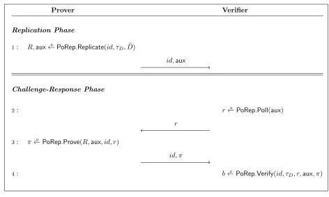
PoRep interactive protocol The PoRep interactive protocol is illustrated in Figure 1. The setup (whether a deterministic, trusted, or transparent public setup) is run externally andppis given as an input to all parties. For each file D, a preprocessor (a special party or the prover when operating in keyless mode, but not the verifier) runs ( ˜D, τD) ← PoRep.Preproc(sk, D). The outputs ˜D, τD are inputs to the prover andτD to the verifier.
-Rational Replication An ideal security goal for PoRep protocols would be to guarantee that any prover who simultaneously passes verification in k distinct PoRep protocols (under k
distinct identities) where the input to PoRep.Replicate is a fileDi in the ith protocol must be storing kindependent replicas, one for each Di, even if several of the files are identical.
Formally, “storing k independent replicas” means that the file can be partitioned into k
Prover Verifier
Replication Phase
1: R,aux←R PoRep.Replicate(id, τ D,D˜)
id,aux
Challenge-Response Phase
2: r←R PoRep.Poll(aux)
r
3: π←R PoRep.Prove(R,aux, id, r)
id, π
4: b←R PoRep.Verify(id, τ
D, r,aux, π)
Figure 2.1: The PoRep interactive protocol is depicted above. The setup and data preprocessing is run externally generatingppand ˜D, τD. The challenge-response protocol is timed, and the verifier rejects any
response that is received more thanT time steps after sending the challenge. This is formally captured by requiringPoRep.Proveto run in parallel time at mostT. A PoRep protocol is a special case of a PoS protocol whereInitializationis the Replication Phase and Executionis the challenge-response phase.
We call this a k-replication of a file. Unfortunately, this security property is impossible to achieve. An adversary can easily “sabotage” its replication storage, e.g. by encrypting it with a key and storing the key separately. This still allows the adversary to decode the original string quickly and otherwise interact with the verifier in exactly the same way.
Instead, a rational model of security is defined in [19]. This security model, called -rational replication roughly says that a PoRep is a µ-sound -rational replication if for any adversary passing the protocol with probability µ there is an “equivalent” adversary who passes with at least the same probability and store a k-replication of the file without incurring more than a 1/(1−) storage overhead (i.e. the adversary saves at most anfraction of its storage by deviating from a k-replication strategy). The security model also accounts for auxiliary information that the adversary might be storing and ensures that the “equivalent” adversary can still extract all the same information from its storage including data unrelated to the PoRep protocol.
Proof of space and PoRC A PoRep is implicitly a publicly verifiable proof of space (Sec-tion 2.2). A prover that passes verifica(Sec-tion in the interactive challenge-reponse protocol for a file ˜D of claimed size |D˜|=N must be using Ω(N) persistent storage. Moreover, a prover that passes verification in k instances of this protocol with distinct ids id1, ..., idk and claimed file
only anspace gap provided that it satisfies-rational replication, and therefore tight proofs of space are necessary for PoReps. A PoRep is also a proof of retrievability of the file D. In fact, sufficient conditions for a (correct) PoRep scheme to satisfy -rational replication are that it is a tight PoS and a PoRC of the data and replica with respect to commitmentsτD and aux. This
was proven (c.f. Lemma 2, [19]) using a knowledge of compression assumption, which roughly says that any prover who knows an algorithm to compress auxiliary data together with the incompressible replica must know an algorithm to compress the auxiliary data independently by the same amount and store the incompressible part separately.
2.4 Graph pebbling games
Pebbling games are the main analytical tool used in graph-based proofs of space and memory hard functions.
Black pebbling game The black pebbling game is a single-player game on a DAGG= (V, E). At the start of the game the player chooses a starting configuration ofP0 ⊆V of vertices that contain black pebbles. The game then proceeds in rounds where in each round the player may place a black pebble on a vertex only if all of its parent vertices currently contain pebbles placed in some prior round. In this case we say that the vertex isavailable. Placing a pebble constitutes amove, whereas placing pebbles on all simultaneously available vertices consumes around. The adversary may also remove any black pebble at any point. The game stops once the adversary has placed pebbles on all vertices in some target/challenge set VC ⊆V.
Pebbling complexity The pebbling game on graph G with vertex set V and target set
VC ⊆V is (s, t)-hard if no player can pebble the set VC in t moves (or fewer) starting from s
initial pebbles, and is (s, t)-parallel-hard if no player can complete the pebbling introunds (or fewer) starting from an initial configuration of at most spebbles. If the hardness holds for any subset containing an α fraction of VC then the pebbling game on (G, VC) is (s, t, α
)-(parallel)-hard.
In a random pebbling game a challenge node is sampled randomly from VC after the player
commits to the initial configuration P0 of s vertices, and the hardness measure includes the adversary’s probability of success. The random pebbling game is (s, t, )-(parallel)-hard if from any s fixed initial pebbles the probability that a uniformly sampled challenge node can be pebbled int or fewer moves (resp. tor fewer rounds) is less than .
Fact 1. The random pebbling game on a DAG G on n nodes with target set VC is (s, t, α) -parallel-hard if and only if the deterministic pebbling game on G with target set VC is (s, t, α) -parallel-hard.
Proof. Fix any P0 of size s. If the random pebbling game on Gwith target set VC is (s, t, α )-parallel-hard then less than an α fraction of the nodes in VC can be pebbled individually in t
rounds starting from P0. Therefore, every subset U in VC of size α|VC| contains at least one
node that cannot be pebbled individually in trounds, hence the (deterministic) pebbling game is (s, t, α)-parallel-hard. Conversely, ifGis (s, t, α)-parallel-hard then less than anα fraction of nodes in VC can be pebbled individually in r rounds. Otherwise, these nodes form a subsetU
that the probability a randomly sampled node from VC can be pebbled in trounds is less than α.
Fact 2. A random pebbling game with a single challenge is (s, t, α)-parallel-hard if and only if the the random pebbling withκ challenges is (s, t, αk)-parallel-hard.
Proof. If the random pebbling game is (s, t, α) hard then by Fact 1 the deterministic pebbling game is (s, r, α) hard, hence there are at most anαfraction of the nodes inVCthat can be pebbled in r rounds from sinitial pebbles. The probability that κ independent random challenges are all nodes from this α fraction is at most ακ. Conversely, if the random pebbling game is not (s, t, α) hard then the adversary can pebble all theκ challenges simultaneously in parallel time
t succeeding on each challenge individually with probability greater than α, hence succeeding on all the challenges with probability greater that ακ.
DAG labeling game A labeling game on a degree d DAG G is analogous to the pebbling game, but involves a cryptographic hash function H : {0,1}dm → {0,1}m, often modeled as
a random oracle. The vertices of the graph are indexed in [n] and each ith vertex associated with the labelci whereci=H(i) ifiis a source vertex, or otherwiseci =H(i||cparents(i)) where
cparents(i) = {cv1, ..., cvd} if v1, ..., vd are the parents of the ith vertex, i.e. the vertices with a
directed edge to vertex i. The game ends when the player has computed all the labels on a target/challenge set of verticesVC. A “fresh” labeling of G could be derived by choosing a salt idfor the hash function so that Hid(x) =H(id||x), and the labeling may be associated with the identifier id.
The complexity of the labeling game (on a fresh identifier id) is measured in queries to the hash function instead of pebbles. This includes the number of labels initially stored, the total number of queries, and the total rounds of sequential queries, etc. The labeling game is (s, r, q, , δ)-labeling-hard if no algorithm that stores initial advice of size sand after receiving a uniform random challenge nodev∈[n] makes a total ofq queries to H inr sequential rounds can output the correct label onvwith probability greater thanover the challengevandδ over the random oracle H.
Random oracle query complexity A general correspondence between the complexity of the black pebbling game on the underlying graphG and the random oracle labeling game is not yet known. However, Pietrzak [33] recently proved an equivalence between the parallel hardness of the randomized pebbling game and the parallel hardness of the random oracle labeling game for arbitrary initial configurations S0 adapting the “ex post facto” technique from [16].
Theorem 1 (Pietrzak [33]). If the random pebbling game on a DAG G with n nodes and in-degreedis(s, r, )-parallel-hard then the labeling game onGwith a random oracleH :{0,1}md→
{0,1}m is(s0, r, , δ, q)-labeling-hard withs0 =s(m−2(logn+ logq))−log(1/δ).
Generic PoS from graph labeling game Many PoS constructions are based on the graph labeling game [18, 33, 35]. Let G(·) be a family of d-in-regular DAGs such that Gn ← G(n) is a d-in-regular DAG on N > n nodes and VC(n) is a subset of n nodes from Gn. Let H:{0,1}dm→ {0,1}mbe a collision-resistant hash function (or random oracle). LetChal(n,Λ)
the labeling game with Gn and target set VC(n) is as follows:
Initialization: The prover plays the labeling game onGn using a hash function Hid =H(id||·). The prover does the following:
1. Computes the labels c1, ..., cN on all nodes of G and commits to them in com using any vector commitment scheme.
2. Obtains vector ofλchallenges ~r←R
Chal(n) from the verifier (or non-interactively derives them using as a seed Hid(com)).
3. For challenges r1, ..., rλ , the prover opens the label on the rith node of Gn, which was
committed incom, as well as the labelscparents(ri) of all its parent nodes. The labels are
added to a listLwith corresponding opening proofs in a list Λ and the prover outputs the proof Φ = (com, L,Λ).
The verifier checks the openings Λ with respect to com. It also checks for each challenge specifying an index v ∈ [N], the label cv in L label and its parent labels cparents(cv), that cv =Hid(v||cparents(cv)). Finally, the prover stores as S only thenlabels inVC.
Execution: The verifier selects κ challenge nodes v1, ..., vκ uniformly at random from VC. The
online prover uses its input S to respond with the label on v and an opening of com at the appropriate index. The verifier can repeat this sequentially, or ask for a randomly sampled vector of challenge vertices to amplify soundness.
Given the correspondence between the hardness of the random oracle labeling game and black pebbling game in the parallel pebbling/computation models, we will focus on parallel pebbling complexity as this is easier to analyze directly.
Red-black pebbling game The soundness of the generic labeling PoS is captured through the red-black pebbling game. An adversary places both black and red pebbles on the graph initially. The red pebbles correspond to incorrect labels that the adversary computes during Initialization and the black pebbles correspond to labels the adversary stores in its advice S. Without loss of generality, an adversary that cheats generates some label that does not require any space to store, which is why red pebbles will be “free” pebbles and counted separately from black pebbles. The adversary’s choice of red pebble placements (specifically how many to place in different regions of the graph) is constrained by theλnon-interactive challenges, which may catch these red pebbles and reveal them to the verifier. The formal description of the red-black pebbling security game for a graph labeling PoS construction withG(n), VC(n), and Chal(n) is
as follows.
Red-Black-PebblesA(G, VC,Chal, t):
1. Aoutputs a set R⊆[N] (of red pebble indices) andS⊆[N] (of black pebble indices).
2. The challenger samplesc1, ..., cλ ←R Chal(n). Ifci ∈Rfor someithenAimmediately loses.
The challenger additionally samples v1, ...., vκ uniformly at random from indices in VC(n)
3. Aplays the random (black) pebbling game onG(n) with the challengesv1, ..., vκ and initial
pebble configurationP0 =R∪S. It runs fortparallel rounds and outputs its final pebble configurationPt. Awins if Pt contains pebbles on all ofv1, ..., vκ.
We formally define PoS soundness for the special case of any graph labeling PoS in terms of complexity of Red-Black-PebblesA(G, VC, t). Let c :N → N denote a cost function c :N → N
representing the parallel time cost (e.g. in sequential steps on a PRAM machine) of computing a label on a node of G(n) for eachn∈N.
Definition 1. A graph labeling PoS with G(n), VC(n),Chal(n) and cost function c(n) is parallel
(s, c(n)·t, µ)-sound if and only if the probability that anyAwinsRed-Black-PebblesA(G, VC,Chal, t)
is bounded by µ where |S|=s.
2.5 Verifiable Delay Encodings
A verifiable delay encoding (VDE) is a non-parallelizable encoding that has high parallel time complexity to compute, but with a fast decoding operation. A VDE may be a special kind of
verifiable delay function [11]. It is more restrictive than a VDF because it must be decodable, but it is less restrictive because the encoding does not need to be unique. Existing pactical (heuristic) examples of VDEs include the Pohlig-Hellmann cipher, Sloth [24], MiMC [3], and a special class of permutation polynomials [11].
Formally, a VDE is a tuple of three algorithmsVDE=VDE.Setup,VDE.Enc,VDE.Decdefined as follows (c.f. [19]).
1. VDE.Setup(t, λ)→pp is given security parameterλand delay parametertproduce public parameters pp. By convention, the public parameters also specify an input space X and a code spaceY. We assume thatX is efficiently samplable. VDE.Setupmight need secret randomness, leading to a scheme requiring a trusted setup.
2. VDE.Enc(pp, x)→y takes an inputx∈ X and produces an outputy∈ Y.
3. VDE.Dec(pp, y)→x takes an inputy∈ Y and produces an outputx∈ X.
Correctness For allppgenerated byVDE.Setup(λ, t) and allx∈ X, algorithmVDE.Enc(pp, x) must run in parallel timetwith poly(log(t), λ) processors, andVDE.Dec(pp,VDE.Enc(pp, x)) =x
with probability 1.
Definition 2 (sequentiality, c.f. [11]). For a function σ(t) a VDE is σ-sequential if for any pair of randomized algorithms A0, which runs in total time O(poly(t, λ)), and A1, which runs
in parallel time t−σ(t) on at most O(poly(t)) processors, the following probability distribution over pp←VDE.Setup(t, λ) is negligible:
P r
"
y← A1(α,pp, x) ∧ y=VDE.Enc(x)
x←R X
α← A0(λ,pp, t) #
<negl(λ)
to proofs of space in order to facilitate incompressibility arguments. We can argue that an algorithm that can use an advice string to succeed with high probability in computing the Encode(pp,·) function in time less than t would be able to compress the function table of a random permutation, similar to how advice string lower bounds are proven in the random oracle model.
Definition 3 (c.f. [19]). An ideal delay permutation (IDP) is a family of oracles {OIDP(t) } that implement a random permutation Π and respond to two types of queries. On a query (q,0) the oracle O(IDPt) internally simulates tsequential queries to Π−1 and then outputs Π(q). On a query
(q,1)it outputs Π−1(q).
2.6 Depth Robust Graphs
A directed acyclic graph (DAG) on n nodes with d-indegree is (n, α, β, d) depth robust graph
(DRG) if every subgraph ofαn nodes contains a path of length at least βn.
Depth robust graph constructions DRGs were first noted by Erd˝os, Graham, and Sze-meredi [32], who constructed a family of (n, α, β, clogn)-depth robust graphs using extreme constant-degree bipartite expander graphs, for some constants α, β, c that satisfy specific con-straints. Mahmoody, Moran, and Vadhan [28] constructed a more flexible family of DRGs that are (n, α, α−, clog2n) depth robust for allα <1. Alwen et. al. [6] recently improved the EGS construction to obtain DRGs for arbitraryα, β as well andO(logn) degree (i.e. with asymptot-ically better degree than MMV). All these constructions still rely on extreme constant-degree expanders (also called local expanders). Explicit constructions of local expanders exist [30], however they are complicated to implement and their concrete practicality is hindered by very large hidden constants. The most efficient way to instantiate these extreme expander graphs is probabilistically. We discuss probabilistic constructions of bipartite expander graphs in Sec-tion 2.7.
A probabilistic DRG construction outputs a graph that is a DRG with overwhelming proba-bility. Instantiating any of the above DRG constructions with probabilistic bipartite expanders results in a probabilistic DRG. However, even probabilistic versions of the above constructions are still not concretely efficient due to their use of local expanders. Alwen et. al. [5] proposed and analyzed the most efficient probabilistic DRG construction to date. The analysis still leaves large gaps between security and efficiency although was shown to resist depth-reducing attacks empirically. Their construction is alsolocally navigatable, meaning that it comes with an efficient parent function to derive the parents of any node in the graph using polylogarithmic time and space.
Definition 4. An (n, α, β, d)-DRG sampling algorithm runs in time O˜(nlogn) and a function DRG.Sample(n, σ) →G that takes an s-bit seed and outputs a graph on n nodes indexed in [n]
such that Gis (n, α, β, d) depth robust graph with probability 1−negl(n) over σ ←R {
2.7 Expander graphs
The vertex expansion of a graph G on vertex set V characterizes the size of the boundary of vertex subsets S ⊆V (i.e. the number of vertices in V \S that are neighbors with vertices in
S).
Definition 5. Let G be an undirected graph on a vertex set V of size n∈N and for any subset
S ⊆V defineΓ(S)to be the set of vertices inV\S that have an edge to some vertex inS. For any constants 0< α < β <1, G is an(n, α, β) expander graph if and only if |Γ(S)∪S| ≥βn for all S of size |S| ≥αn. For anyδ >0, the set S is called(1 +δ)-expanding if|Γ(S)∪S| ≥(1 +δ)|S|.
In the case of directed bipartite graphs, vertex expansion is defined by the minimum number of sources connected to any given number of sinks.
Definition 6. For any constants α, β where 0 < α < β < 1 and integer n ∈ N, an (n, α, β)
bipartite expander is a directed bipartite graph with n sources and n sinks such that any subset of αn sinks are connected to at least βn sources. For any δ >0, a subset S of sinks is called
(1 +δ)-expanding if it is connected to at least (1 +δ)|S| sources.
It is easy to construct an undirected expander graph given a bipartite expander as defined above.
Claim 1. LetH be a(n, α, β) bipartite expander graph with bounded degreed, sources and sinks labeled by indices in [n] and edge set E⊆[n]×[n]. Define the undirected graph G with vertices labeled in [n] and edge set E0 such that (i, j) ∈ E0 (for i 6= j) if and only if (i, j) ∈ E or
(j, i)∈E. Then G has bounded degree 2dand is an (n, α, β) expander.
Proof. Every vertex in G has at most degree 2d because H has bounded degree d, and the number of edges added to any node indexed with label iinG is at most the sum of number of edges incident to theith source andith sink inHrespectively. Now consider any subsetS⊆[n] of αn vertices in G. S also corresponds to a subset of the sources in H with the same index labels and is connected to at leastβnsinksT ⊆[n]. For eachs∈S andt∈T wheres6=tthere is an edges (s, t) in G. Therefore, Γ(S) =T \S and |Γ(S)| ∪S=|T| ≥βn.
Given this equivalence, for the remainder of this section we focus on constructions of constant degree bipartite expanders.
Constructing bipartite expanders There is a rich literature on constructions of bipartite expanders, and includes both explicit and randomized constructions of constant degree bipartite graphs with very good expansion properties. The randomized construction of Chung [15] simply defines the edges of ad-regular bipartite expander on 2nvertices by connecting thednoutgoing edges of the sources to the dn incoming edges of the sinks via a random permutation Π : [d]×[n]→[d]×[n]. More precisely, the ith source is connected to the jth sink if there is some
Lemma 1 (RD [35]). The Chung random bipartite graph construction is a d-regular (n, α, β)
expander with probability 1−negl(nHb(α)) for alld, α, β satisfying:
Hb(α) +Hb(β) +d(βHb(α/β)−Hb(α))<0 (2.1)
where Hb(x) =−xlog2x−(1−x) log2(1−x) is the binary entropy function.
For example, the above formula shows that for α= 1/2 and β= 0.80 Chung’s construction gives an (n,0.5,0.80) expander ford≥8, meaning any subset of 50% of the sinks are connected to at least 80% of the sources when the degree is at least 8.
Expansion vs subset size In general, the expansion factor (the ratio β/α) improves in smaller subsets: if a given expansion factor holds with overwhelming probability in large subsets then it also holds with overwhelming probability in smaller subsets. On the other hand, the absolute expansionβ is monotonically non-decreasing as a function ofα because the expansion of any set is at least the expansion of its subsets.
Lemma 2. For any k > 1 and d > 2, if the output of Chung’s construction is a d-regular
(n, α, kα)bipartite expander for someα < dk−(dk−−2)1 with probability1−negl(nHb(α))thenβG(α0)≥ kα0 for every subset of size α0 < αwith probability 1−negl(nHb(α0)).
Proof. For fixed dandk defineφ(α) =Hb(α) +Hb(kα) +dkαHb(1/k)−dHb(α). By Lemma 1,
Chung’s construction outputs a graph that is a d-regular (n, α, kα) bipartite expander with probability 1−negl(nHb(α)) as long as φ(α) < 0. We will show that if φ(α) < 0 for some
α within the domain X = (0,dk−(dk−−2)1), then φ(α0) < 0 for all α0 < α. We will first prove two subclaims:
1. φis smooth onα∈(0,1/k) (i.e. twice differentiable), and limα→0φ= 0.
2. φis decreasing at α= 0 (i.e. increasing in the limitα→0) and convex onX.
Together these imply that if φ(α) < 0 for α ∈ X then φ(α0) < 0 for all α0 < α. Suppose not, then there exists some point α0 < α such that φ(α0) ≥ 0 > φ(α). Since φ is continuous on X and initially negative and decreasing it must increase on some subinterval of (0, α0) and then decrease again on some subinterval of (α0, α). However, this contradicts the fact thatφis convex onX, and hence once it starts increasing at any point inX it will not decrease again in any higher interval.
Proof of subclaim 1: φ is a linear combination of Hb(α), Hb(kα), and α, which are all real and twice differentiable on (0,1/k). In particular, H0(α) = log2(1−α)−log2(α) and H00(α) =
−1
log2(e)α(1−α). Finally, limα→0Hb(α) = limα→0Hb(kα) = 0, hence the limitα → 0 of any linear
combination of Hb(α), Hb(kα), andα is 0.
Proof of subclaim 2: We first show that limα→0φ0=−∞. Note thatφ0(α) =Hb0(α) +kHb0(αk) +
dkHb(1/k)−dHb0(α). Asα→0 the limit is determined by the terms involvingH
0
b(α) andH
0(αk),
which go to−∞whiledkHb(1/k) is constant. SincekHb0(αk)−(d−1)Hb0(α) =k(log2(1−αk)− log2(αk))<−klog2(αk)−(d−1)Hb0(α) we get:
lim
α→0φ
0 < lim
Now looking at the second derivative, φ00(α) =k2Hb00(αk)−(d−1)H00(α):
φ00(α) = −1 log2(e)α
k
1−αk + d−1 1−α
Hence φ00 > 0 if and only if (d−1)(1−αk) > k(1−α). Rearranging the equation, we get
α < dk−(dk−−2)1.
Corollary 1. For d = 8 Chung’s construction is an 8-regular bipartite graph such that every subset of at most 1/3 of the nodes is 2-expanding, i.e. it is an (n, α,2α)-bipartite expander for every α≤1/3 with overwhelming probability.
Proof. Pluggingα= 1/3 andβ = 2/3 into the formula for degree (Equation 2.1) givesd= 7.21<
8. Withd= 8 andk= 2 the condition in Lemma 2 is satisfied: α= 1/3<(d−k−1)/k(d−2) = 5/12.
For fixed d the expansion improves further as α decreases. One can easily verify (by re-peated application of L’Hopital’s rule) that the limit as α → 0 of the expression (Hb(α) + Hb(kα))/(Hb(α)−kαHb(1/k)) goes to k+ 1. Of course, when α becomes too small the
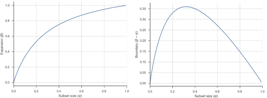
expan-sion no longer holds with overwhelming probability. Figure 2.2 provides a table of expanexpan-sion factors over a range of α with fixed degree d= 8. Figure 2.3 plots the expansion as a function of subset size.
Expansion boundary In the analysis of our constructions we will also look at the boundary
of subsets in an expander graph. In an undirected expander, this is simply Γ(S) as we defined already. In the case of bipartite expanders, the analogous “boundary” of a set of sources is the set of sinks connected to these sources that have distinct index labels from the sources. We can lower bound the size of the boundary byβ−α. Lemma 1 gives a smooth lower bound onβ−α
for Chung’s bipartite expander graphs that we can show has a unique local maximum in (0,1). Conveniently, this allows us to lower bound the value ofα−β in any given range by examining just the end points. In particular, when d = 8 this achieves a local max at approximately
α= 1/3 (where the expansion factor reaches 2), which can be seen in Figure 2.3. We prove the claim analytically for arbitrary d.
To simplify the analysis, we look at the function defined by the zeros ofφ(α, β) =d(βHb(α/β)−
Hb(α)) + 2 = 0. Anyα, β satisfying this relation also satisfies the relation in Lemma 1 because Hb(α) +Hb(β) < 2 when β > α. (More generally we can substitute c if it is known that Hb(α) +Hb(β) < c). This implicitly defines β as a function of α, as well as the function
ˆ
β =β−α. More precisely, The implicit function ˆβ(α) defined by pairs of points (α,βˆ(α)) such that φ(α, α+ ˆβ(α)) = 0 is a lower bound to the boundary of subsets of size α, which holds at any point α with probability at least 1−negl(nHb(α)).
Lemma 3. Define φ(x, y) =d(yHb(x/y)−Hb(x)) +c where c is any constant and let βˆ be the function on(0,1)defined by pairs of points(α, β−α) such that φ(α, β) = 0and 0< α < β <1. The function βˆ is continuously differentiable on (0,1)and has a unique local maximum.
Proof. Define a change of variablesz=x−yto getφ(x, z) =d(x+z)Hb(x/(x+z))−Hb(x)) +c
φ(x, z) is continuously differentiable in both variables on the set (0,1)×(0,1), i.e. its partial derivates φz= ∂φ∂z and φx= ∂φ∂x are each continuous on (0,1)×(0,1). By the Implicit Function
Theorem, ˆβ : (0,1) → R is continuously differentiable with derivative −φx/φz defined in an
open interval around every point α where φz 6= 0. Expanding the binary entropy function
Hb(x) =−xlog2(x)−(1−x) log2(1−x) simplifies the inner expression:
1
d(φ(x, z)−c) = (z+x)Hb(x/(x+z))−Hb(x)
=−xlog2(x/(z+x))−zlog2(z/(x+z)) +xlog2(x)−(1−x) log2(1−x)
= (x+z) log2(x+z)−zlog2(z)−(1−x) log2(1−x)
The partial derivatives are:
φx= d
ln(2)((x+z)/(x+z) + ln(x+z)−(1−α)/(1−α)−ln(1−α) =dlog2
x+z
1−α
φz= d
ln(2)((x+z)(x+z) + ln(x+z)−z/z−ln(z) =dlog2
x+z z
φz(α,βˆ(α)) is always positive because (x +z)/z > 1 for x, z ∈ (0,1). On the other hand,
φx(α,βˆ(α) < 0 if and only if α+ ˆβ(α) > 1−α. Setting ˆβ(α) = β −α this is the case when β+α >1. ˆβ(α) is increasing whenα+β < 1 and decreasing whenα+β > 1. It has a local maximum where α+β = 1. Since β = ˆβ(α)−α is a monotonically non-decreasing function of
α it follows that if α+β <1 then α0+β0 < 1 at every point α0 < α. Likewise, if α+β >1 then α0+β0 >1 at every point α0 > α. We therefore conclude that ˆβ(α) is initially increasing and achieves a unique local maximum on (0,1).
Corollary 2. With overwhelming probability in n, Chung’s construction (with d = 8) is an
8-regular bipartite graph on n sinks and n sources each indexed in [n] such that for all α ∈ (0.10,0.80) every αn sinks are connected to at least 0.12n sources with distinct indices.
Proof. The function ˆβ(α) from Lemma 3 the implicit function ˆβc defined by pairs of points
(α, β −α) satisfying φc(α, β) = d(βHb(α/β)−Hb(α)) +c = 0 is a smooth and has a unique maximum in any intervalL⊆(0,1). Furthermore, if the pointsαandβ satisfyHb(α) +Hb(β)< c≤2 then ˆβ(α) is a lower bound on the “boundary” of sinks of sizeαn in Chung’s construction with overwhelming probability (Lemma 1). We will split the interval (0.10,0.80) into subintervals (0.10,0.33] and [0.33,0.80) and analyze them seperately.
For allα∈[0.33,0.80) the formula in Lemma 1 shows that the expansion for each α is non-decreasing and is at least 0.80 (see Figure 2.3). Thus we can setc= 1.64> Hb(0.33) +Hb(0.80)
and examine the lower bound ˆβc. It has a unique local maximum in (0.33,0.80) therefore ˆ
βc ≥ min( ˆβc(0.33),βˆc(0.80)) ≥ 0.12. (Observe that φc(0.33,0.45) < 0 and φc(0.80,0.92) < 0
withd= 8.)
Size(α) 0.01 0.10 0.20 0.30 0.40 0.45 0.50 0.55 0.60 0.65 0.70 0.75 0.80
Expansion(β) 0.04 0.33 0.53 0.65 0.75 0.78 0.81 0.84 0.88 0.89 0.91 0.93 0.94
Factor(β/α) 4 3.3 2.65 2.1 1.8 1.73 1.62 1.53 1.47 1.37 1.3 1.24 1.17
Figure 2.2: A table of the maximum expansion (β) satisfying the condition from Lemma 1 for Chung’s con-struction with fixed degreed= 8 over a range of subset sizes (α).
Figure 2.3: The graph on the left plots the lower bound from Lemma 1 on the expansionβas a function of the subset sizeα(in fractions of the sources/sinks) for Chung’s construction with fixedd= 8. The graph on the right plots the corresponding lower bound on β−α, which is the analog of the subgraph boundary in non-bipartite expanders. Specifically, this is a lower bound on the fraction of sinks connected to anαfraction of sources that have distinct index labels from the sources.
Expansion vs degree We can also characterize the expansion of subsets of the sinks more generally as a function of the graph’s degree. We can show that for anyd≥4 Chung’s construc-tion yields ad-regular graph such that every subset of sinks of sizeαnis at least (d/3)-expanding forevery α < 23d.
Lemma 4. For any d≥ 4, Chung’s construction yields a d-regular bipartite graph that is an
(n, α,(d/3)α) bipartite expander for everyα ≤ 23d with probability 1−negl(nHb(α)).
Proof. First set α = 3/(2d) and β = 1/2. By Lemma 1, we obtain a graph G that is an (n, α, β) expander with probability 1−negl(nHb(α)) as long as d− d2Hb(3d)−Hb(23d)−1> 0. Defineg(x) = 1/x− 1
2xHb(3x)−Hb(3x/2)−1 so that the condition is equivalent tog(1/d)>0. Hb(x) is real and continuous on (0,1). Its derivative is Hb0(x) = log2(1−x)−log2(x) which is positive on (0,1/2). Differentiating g(x) with respect to x on (0,1/3) gives g0(x) = −1/x2 −
3 2xH
0
b(3x)+2x12Hb(3x)−32Hb0(32x). Observe that on (0,1/3) bothH
0
b(3x)>0 and 12Hb(3x)−1<0, therefore g0(x)<0. This means thatg(1/d) is increasing as dincreases ford >3. Furthermore limd→3g(1/d) = 3−Hb(1/2)−1 = 1>0.
Finally, it follows as a special case of Lemma 2 that if G is a d-regular (n,23d,12) bipartite expander for some fixeddthen it is an (n, α,(d/3)α) bipartite expander for everyα≤ 3
Ramanujan graphs The explicit bipartite expander construction of Lubotzky, Phillips, and Sarnak [4] achieves similar expansion to Chung’s construction for similarly good parameters. It is more complicated to implement as it involves generating a certain Cayley graph of the group P GL(2,Fq), the 2-dimensional projective general linear group onFq. This construction
yields a bipartite exapnder of degree (p+ 1) on q(q2−1) vertices for any primes p, q such that
p, q ≡ 1 mod 4 and p is a quadratic non-residue modulo q. The resulting graph is called a
Ramanujan graph because it is an optimal spectral expander, meaning the absolute value of all the non-trivial eigenvalues of its adjacency matrix (i.e. except the eigenvalue -d) are bounded by 2√d−1. Other explicit Ramanujan graphs are known, for instance the isogeny graph of supersingular elliptic curves is also Ramanujan [34]. Due to a theorem of Tanner [38] relating spectral and vertex expansion, any d-regular bipartite Ramanujan graph on n vertices is an (n, α,4(1−αd)+αd) bipartite expander for all α < 1. In particular, for d ≥ 4 every fraction of
α <1/dsinks is at leastd/4-expanding.
Lemma 5 (Tanner [38]). For any d≥4 and n∈N a d-regular bipartite Ramanujan graph on n vertices is an (n, α,(d/4)α) bipartite expander for every α <1/d.
3
Stacked DRG Proof of Space
In this section we show that stacking DRGs with bipartite expander edges between layers yields an arbitrarily tight proof of space with the number of layers increasing asO(log2(1/)) where
is the desired space gap. Moreover, the proof size is also O(log2(1/)), which is asymptotically optimal. Our proofs attempt a tight analysis as well, e.g. showing that just 10 layers achieve a PoS with a 1% space gap, degree 8 +dgraphs wheredis the degree of the DRG, and relies only on a DRG that retains depth in 80% subgraphs.
3.1 Review of the Stacked-Expander PoS
In this section we review the PoS construction by Ren and Devadas [35] based on stacked bipartite expander graphs as it is a building block towards ourLayered-DRGconstruction. Their construction uses a layered graph where each layer is a directed line onnnodes and the directed edges of a bipartite expander graph are placed between layers. This was shown to be an (γn,(1− 2)γn)-sound PoS for parameters <1/2 and γ <1.3 (Achieving practical proof sizes actually requires γ to be rather small as otherwise the required degree of the expander graphs blows up, e.g. γ > 0.6 requires at least degree 40 graphs hence practically < 1/3). The PoS is not parallel sound (for meaningful s, t) as a prover running in O(λ) parallel time can pass verification using very little space. We will show that by replacing each line graph with a depth robust graph this results in a much tighter proof of space, as well as security against parallelism. Interestingly, the security against parallel attacks seems intimately connected to why the Ren-Devadas construction fails to be tight whereas ours succeeds. Furthermore, the Ren-Ren-Devadas security is only proven against an adversary who implements a pebbling attack and is not yet known to be secure more generally against graph labeling in the random oracle model. As our
3
construction is secure against parallel pebbling attacks it is also secure in the random oracle model.
The graph GSE The stacked-expander PoS uses the same underlying graph as the Balloon
Hash memory hard function [22]. The graphGSE consists of`=O(λ) layersV1, ..., V` consisting
each ofnvertices indexed in each level by the integers [n], and whereλis a security parameter. First directed edges are placed from each kth vertex to the k+ 1st vertex in each level, i.e. forming a directed line. Next directed edges are placed from Vi−1 to Vi according to the edges of an (n, α, β) bipartite expander on (Vi−1, Vi). Finally a “localization” operation is applied so
that each kth vertexuk inVi−1 is connected to the kth vertex vk inVi and any directed edge from the kth vertex of Vi−1 to some jth vertex of Vi where j > k is replaced with a directed edge from the kth vertex of Vi to the jth vertex of Vi. GSE can be pebbled inn` steps using a
total of npebbles.
Stacked-expander PoS The PoS follows the generic PoS based on graph labeling. We remark only on several nuances. Due to the topology of GSE after localization, the prover only needs to use a buffer of size n and deletes the labels of Vi−1 as it derives the labels of Vi. After
completing the labels Ci in theith level it computes a vector commitment (e.g. Merkle) to the labels in Ci denoted comi. Once it has derived the labels C` of the final level V` it computes com = Hid(com1|| · · · ||com`) and uses Hid(com||j) to derive λ non-interactive challenges for
each jth level.4
Letγ=β−2αfor constantsβ, α∈(0,1) whereβ >2α. For the remainder of the analysis we assume the bipartite expander graph used in the stack-expander PoS construction is an (n, α, β) expander.
Theorem 2(RD [35]). Let`be the number of layers inGSE andα, β the expansion parameters. Let γ =β−2α. Every αn subset of initially unpebbled sinks in the layerV` cannot be pebbled in less than 2`αn moves from any initial configuration ofγn and using at mostγn pebbles overall.
Corollary 3(RD [35]). For every <1/2and0< δ < γarbitrarily small, the stacked-expander PoS construction is an ((γ−δ)nm,(1−2)γn)-sound PoS (against a pebbling adversary) with probability 1−negl(δλ).
Space-hardness gap 1/2 The stacked-expander PoS leaves at least a 12γ gap between the honest prover’s storage and the adversary’s storage. In fact, the space gap itself is actually what the analysis exploits in order to argue security: due to the fact that the adversary will need to refill a large fraction of its deleted space in order to pass the verifier’s challenges it will end up performing a significant amount of computation as well to refill that space. Furthermore,
4
This is a slight deviation from the protocol as described by Ren and Devadas, which sampled every label challenge randomly over all vertices inGSE rather than separately within each layer. The end result is the same because for security they set their parameters to ensure that if at leastnlabelsin any level are incorrect (which comprise an/` fraction of all the vertices) then the challenges will sample one of these incorrect labels with overwhelming probability. This requires sampling a factor `more labels overall than the number of labels one would sample from a given level to achieve the same probability of detection within that specific layer, as for any λit holds that (1−
`)
Corollary 3 proves that nodes on the last level are hard to pebble individually by leveraging the fact that the adversary is storing less than half the pebbles required to pebble a subset of nodes (as required by Theorem 2) and derives a contradiction by considering a lazy adversarial strategy that keeps these pebbles fixed on the initial set and still uses less space than needed. This analysis would be void if the adversary were storing more than half the required online pebbles.
It seems implicitly that the reason this bound on additional online space used is so fun-damental to the analysis is that the protocol is not secure against parallel attacks. If instead pebbling any αn sinks was secure against parallel attacks (with no bound on the number of online pebbles used in parallel) then we immediately get that less thanαnsinks can be pebbled efficiently individually as otherwise these could all be pebbled in parallel starting from the same initial configuration.
O(λ2) proof size The proof size in the stacked-expander PoS is quite large as it requires λ
challenges in each of the λlevels for total complexity O(λ2). The number of levels needs to be
λas we are only able to prove that the complexity of pebbling a single node out of αn sinks is at least 1/(αn) the complexity of pebbling all αn, hence the complexity of pebblingαn nodes needs to be on the order of 2λαn, i.e. much greater than O(n). If the complexity were only
O(n) the adversary might be able to pebble each challenge in less that 1/αmoves. Again, this is connected to the lack of security against parallel attacks. If the protocol were secure against parallel attacks then individual nodes inherit the pebbling complexity of αn nodes without a factor αn loss.
3.2 A tight PoS from stacked DRGs
The new result that we will next show is that simply replacing each of the line graphs Vi in
the stacked-expander PoS construction with a depth robust graph results in an arbitrarily tight PoS. Specifically, only O(log 1/) layers are needed to achieve a ((1−)n,Ω(n))-parallel-sound PoS. We demand only very basic properties from the DRG, e.g. that any subgraph on 80% of the nodes contains a long path of Ω(n) length.
Construction ofGSDR[`] The graphGSDR[`] will be exactly likeGSE only each of the`layers V1, ..., V` contains a copy of an (n,0.80n, βn)-depth-robust graph for some constant β. For
concreteness, we define the directed edges between the layers using the degree 8 Chung random bipartite graph construction.
For simplicity we will first analyze the construction without applying localization to the expander edges between layers. Even without localization this is already a valid PoS, only the initialization requires a buffer of size 2nrather than n. The PoS is still “tight” with respect to the persistent space storage.
Vector commitment storage If the vector commitment storage overhead required for the PoS is significant then this somewhat defeats the point of a tight PoS. Luckily this is not the case. Most vector commitment protocols, including the standard Merkle tree, offer smooth time/space tradeoffs. With a Merkle tree the honest prover can delete the hashes on nodes on the first k levels of the tree to save a factor 2k space and re-derive all hashes along a Merkle
1% overhead in space, and requires at most 128 additional hashes and reads. Furthermore, as remarked in [33] these 2k reads are sequential memory reads, which in practice are inexpensive
compared to the random reads for challenge labels.
Proof size We show that`=O(log(3(−12δ))) suffices to achievenegl(λ) soundness against any prover running in parallel time less than βn rounds of queries where Chal samples λ/δ nodes in each layer. This would result in a proof size of O((1/) log(1/)), which is already a major improvement on any PoS involving a graph of degree O(1/) (recall that the only previously known tight PoS construction relied on very special DRGs whose degree must scale with 1/, which results in a total proof size of O(1/2)). However, we are able to improve the result even further and show that only O(1/δ) challenge queries are required overall, achieving proof complexity O(1/). This is the optimal proof complexity for the generic pebbling-based PoS with at most an space gap. If the prover claims to be storingnpebbles and the proof queries less than 1/ then a random deletion of an fraction of these pebbles evades detection with probability at least (1−)1/ ≈1/e. The same applies if a random fraction of the pebbles the prover claims to be storing are red (i.e. errors).
Analysis outline We prove the hardness of the game Red-Black-PebblesA(GSDR[`], V`,Chal)
whereChalsamplesλi uniform challenges over Vi. We first show that it suffices to consider the
parallel complexity of pebbling the set U` ⊆ V` of all unpebbled nodes on V` from an initial configuration ofγnblack pebbles overall andδinred pebbles in each layer whereδ`< /2. As a
shorthand notation, we will say thatGSDR[`] is (γ, ~δ, t, µ)-hard iftrounds are required to pebble a µ fraction ofV`. When µ = 1 this is equivalent to pebbling all of U`, the set of nodes with missing pebbles in the initial configuration (since there is no constraint on number of pebbles used). This very similar to standard parallel pebbling complexity in black pebbling games as we defined earlier, however, it takes into account the restriction to δi red pebbles on each layer that it counts separately5 from black pebbles.
In Claim 4 we show that if GSDR[`−1] is (1−+ 2δ`−1, ~δ, t,1)-hard then GSDR[`] is (1− , ~δ∗, t,1 −/2)-hard where ~δ∗ is equal to ~δ on all common indices and δ` = δ`−1. This in
turn implies that with probability at least 1−/2 a randomly sampled challenge node from V`
requires more thantrounds to pebble. Together with the random challenges boundingδiwe show
(Claim 2) that the labeling PoS onGSDRis (γn, t, max{p∗, µκ})-sound wherep∗=maxi(1−δi)λi.
Next we look at the complexity of pebbling all of V`. We show in Claim 6 that when the
adversary uses at mostγ <1−black pebbles andδ red pebbles in each layer then pebbling all the unpebbled nodes in layerV` (for`dependent onandδ) requires pebbling 0.80nunpebbled nodes (including both red and black pebbles) in some layer Vi. Since the layer Vi contains a (n,0.80, βn)-depth-robust graph, this takes at leastβnrounds. We then generalize this analysis (Claim 7) to apply when δi is allowed to increase from level ` to 1 by a multiplicative factor such thatP
iδi=O(δ`).
Theorem 3 ties everything together, taking into account the constraints of each claim to derive the PoS soundness of the labeling PoS on GSDR[`].
5