Function Secret Sharing: Improvements and Extensions
∗
Elette Boyle
†Niv Gilboa
‡Yuval Ishai
§July 24, 2018
Abstract
Function Secret Sharing (FSS), introduced by Boyle et al. (Eurocrypt 2015), provides a way for additively secret-sharing a function from a given function family F. More concretely, an
m-party FSS scheme splits a functionf :{0,1}n→
G, for some abelian groupG, into functions
f1, . . . , fm, described by keysk1, . . . , km, such thatf =f1+. . .+fmand every strict subset of
the keys hidesf. A Distributed Point Function (DPF) is a special case whereFis the family of point functions, namely functionsfα,β that evaluate toβ on the input αand to 0 on all other inputs.
FSS schemes are useful for applications that involve privately reading from or writing to distributed databases while minimizing the amount of communication. These include different flavors of private information retrieval (PIR), as well as a recent application of DPF for large-scale anonymous messaging.
We improve and extend previous results in several ways:
• Simplified FSS constructions. We introduce a tensoring operation for FSS which is used to obtain a conceptually simpler derivation of previous constructions and present our new constructions.
• Improved 2-party DPF.We reduce the key size of the PRG-based DPF scheme of Boyle et al. roughly by a factor of 4 and optimize its computational cost. The optimized DPF significantly improves the concrete costs of 2-server PIR and related primitives.
• FSS for new function families. We present an efficient PRG-based 2-party FSS scheme for the family ofdecision trees, leaking only the topology of the tree and the internal node labels. We apply this towards FSS for multi-dimensional intervals. We also present a general technique for obtaining more expressive FSS schemes by increasing the number of parties.
• Verifiable FSS. We present efficient protocols for verifying that keys (k1∗, . . . , k∗m),
ob-tained from a potentially malicious user, are consistent with some f ∈ F. Such a ver-ification may be critical for applications that involve private writing or voting by many users.
Keywords: Function secret sharing, private information retrieval, secure multiparty com-putation, homomorphic encryption
∗
This is a full version of [10]. †
IDC Herzliya, Israel,[email protected]. ‡
Ben Gurion University, [email protected]. §
1
Introduction
In this work we continue the study of Function Secret Sharing (FSS), a primitive that was recently introduced by Boyle et al. [8] and motivated by applications that involve private access to large distributed data.
Let F be a family of functionsf :{0,1}n →
G, where Gis an abelian group. Anm-party FSS scheme for F provides a means for “additively secret-sharing” functions from F. Such a scheme is defined by a pair of algorithms (Gen,Eval). Given a security parameter and a description of a function f ∈ F, the algorithm Gen outputs an m-tuple of keys (k1, . . . , km),
where each keykidefines the functionfi(x) =Eval(i, ki, x). The correctness requirement is that
the functionsfi add up tof, where addition is inG; that is, for any inputx∈ {0,1}n we have that f(x) =f1(x) +. . .+fm(x). The security requirement is that every strict subset of the
keys computationally hidesf. A naive FSS scheme can be obtained by additively sharing the entire truth-table off. The main challenge is to obtain a much more efficient solution, ideally polynomial or even linear in the description size off.
The simplest nontrivial special case of FSS is aDistributed Point Function(DPF), introduced by Gilboa and Ishai [24]. A DPF is an FSS for the family of point functions, namely functions
fα,β : {0,1}n →
G for α ∈ {0,1}n and β ∈ G, where the point function fα,β evaluates to β on input αand to 0 on all other inputs. Efficient constructions of 2-party DPF schemes from any pseudorandom generator (PRG), or equivalently a one-way function (OWF), were presented in [24, 8]. This was extended in [8] to more general function families, including the family of
interval functions f[a,b] that evaluate to 1 on all inputsx in the interval [a, b] and to 0 on all other inputs. Form ≥3, the best known PRG-based DPF construction is only quadratically better than the naive solution, namely the key size grows linearly with√N whereN = 2n [8].
We consider here the casem= 2 by default.
On the high end, efficient FSS schemes for arbitrary polynomial time functions can be based on the Learning with Errors (LWE) assumption by using threshold or key-homomorphic variants of fully homomorphic encryption [8, 18]. (Alternatively, they can be based on indistinguisha-bility obfuscation and one-way functions [8].) In the mid-range, FSS schemes for log-space or NC1 functions (with inverse polynomial error) are implied by the Decisional Diffie-Hellman as-sumption [9]. In the present work we mainly consider PRG-based FSS schemes, which have far better concrete efficiency and are powerful enough for the applications we describe next.
FSS schemes are motivated by two types of applications: ones that involve privatelyreading
from a database held bymservers, and ones that involve privatelywriting(or incrementing) an array which is secret-shared amongmservers. In both cases, FSS can be used to minimize the communication complexity. We illustrate two concrete application scenarios below and refer the reader to Appendix A for more details and additional examples.
For a typical “reading” application, consider the problem of 2-server Private Information Retrieval (PIR) [14, 12]. In the basic flavor of 2-server PIR, the two servers hold a database of
N strings (x1, . . . , xN), wherexi∈ {0,1}`, and a client wishes to retrievexαwithout revealing α to either of the two servers. PIR in this setting can be implemented by having the client distribute the point function fα,1 : [N] → Z2 between the servers. Concretely, the client generates a pair of keys (k1, k2) which define additive sharesf1, f2 of fα,1, and sends each key to a different server. On input ki, server isends back the sum PN
j=1xjfi(j), where eachxj is viewed as an element in Z`
2. The client can recover xα by taking the exclusive-or of the two `-bit strings it receives. See Appendix B for a survey of alternative approaches to PIR.
incur a significant additional overhead in round complexity, storage, and cost of updates [13]. In general, FSS for a function familyFcan be directly used to perform private searches defined by predicates fromF. By additionally using data structures and coding techniques, data structures and coding techniques, the power of FSS for simple function families F can be significantly boosted. For instance, the recent “Splinter” system [38] efficiently supports a rich class of private search queries by building only on FSS schemes for point functions and interval functions.
For a typical “writing” application, consider the following example from [8]. Suppose that we want to collect statistics on web usage of mobile devices without compromising the privacy of individual users, and while allowing fast collection of real-time traffic data for individual web sites. A DPF provides the following solution. An array of counters is additively shared between 2 servers. A client who visits URLαcan now secret-share the point function f =fα,1 over a sufficiently large groupG=ZM intof =f1+f2. Each serveriupdates its shared entry of each URLαj by locally addingfi(αj) to its current share ofαj. Note that the set of URLsαj used
to index entries of the array does not need to include the actual URLαvisited by the client, and in fact it can include only a selected watchlist of URLs which is unknown to the client. A different “writing” application for DPF was proposed in the context the Riposte system for anonymous messaging [15]. In this system, messages from different clients are mixed by having each client privately write the message to a random entry in a distributed array.
1.1
Our Contribution
Motivated by applications of FSS, we continue the study of efficient constructions that can be based on any PRG. We improve and extend previous results from [8] in several directions.
Simplified FSS constructions. We introduce a conceptually simple “tensoring” operation
for FSS, which we use both to rederive previous constructions and obtain some of the new constructions we describe next.
Improved 2-party DPF. We reduce the key size of the PRG-based DPF scheme from [8]
roughly by a factor of 4 and optimize its computational cost. In an AES-based implementation, the key size of a DPF is equivalent to roughly a single AES key per input bit. We provide further optimizations for the case of DPF with a single-bit output and for reducing the computational cost of evaluating the DPF on the entire domain (as needed, for instance, in the PIR application described above). The optimized DPF can be used to implement 2-server PIR protocols in which the communication overhead is extremely small (e.g., roughly 2.5K bits are sent to each server for retrieving from a database with 225 records) and the computation cost on the server side is typically dominated by the cost of reading and computing the XOR of half the data items. More concretely, the additional computational cost of expanding the DPF key for anN-record database consists of roughly N/64 AES operations. In the case of private keyword search, retrieving the payload associated with an 80-bit keyword requires the client to send less than 10Kbits to each server, and each server to send back a string of the same length as the payload. The server computation in this case is dominated by 73 AES invocations per keyword. See Table 1 for more details on the concrete efficiency of our DPF construction and Appendix B for more details on the PIR application and a comparison with alternative approaches from the literature.
products of pairs of functions from two given families that are realized by FSS. This can be applied towards more efficient solutions for multi-dimensional intervals, though with a larger number of parties.
Verifiable FSS.In both types of applications of FSS discussed above, badly formed FSS keys
can enable a malicious client to gain an unfair advantage. The effect of malicious clients can be particularly devastating in the case of “writing” applications, where a single badly formed set of keys can corrupt the entire data. We present efficient protocols for verifying that keys (k∗1, . . . , k∗m) are consistent with some f ∈ F. Our verification protocols make black-box use of the underlying FSS scheme, and avoid the cost of general-purpose secure computation tech-niques. The protocols make a novel use of sublinear verification techniques (including special-purpose linear sketching schemes and linear PCPs) and combine them with MPC protocols that exploit correlated randomness from an untrusted client for better efficiency. These techniques may be applicable beyond the context of verifiable FSS.
A verification protocol for DPF was previously proposed in the context of the Riposte system for anonymous messaging [15]. Compared to our verification protocols, the protocol from [15] requires an additional party, its communication complexity is higher, and it only applies to a special (and relatively inefficient) DPF implementation.
Organization. Useful definitions appear in Section 2. Several FSS constructions, including
the tensor product generalization, optimized DPF and evaluating a DPF on the entire domain, are presented in Section 3. Definitions and protocols for verifiable FSS are the focus of Section 4. The appendices contain further discussion on applications of FSS and the concrete efficiency of PIR, as well as some proofs.
2
Preliminaries
We extend the definition of function secret sharing from [8] by allowing a general specification of the allowable leakage, namely the partial information about the function that can be revealed. We also give a more explicit treatment of how functions and groups are represented.
Modeling function families. A function family is defined by a pair F = (PF, EF), where
PF⊆ {0,1}∗ is an infinite collection of function descriptions ˆf, andEF :PF× {0,1}∗→ {0,1}∗ is a polynomial-time algorithm defining the function described by ˆf. Concretely, each ˆf ∈PF describes a corresponding function f : Df →Rf defined by f(x) = EF( ˆf , x). We assume by default thatDf ={0,1}n for a positive integer n(though will sometimes consider inputs over
non-binary alphabets) and always requireRf to be a finite Abelian group, denoted byG. When there is no risk of confusion, we will sometimes write f instead of ˆf and f ∈ F instead of
ˆ
f ∈PF. We assume that ˆf includes an explicit description of bothDf andRf as well as a size parameterSfˆ.
Representing groups and their elements. We restrict the attention to Abelian groups Gof the form Zu1× · · · ×Zu`, for positive integers u1, . . . , u`, and represent such a group by
the sequence (u1, . . . , u`). A group element y ∈ G is naturally described by a sequence of ` non-negative integers.
Modeling leakage. We capture the allowable leakage by a functionLeak:{0,1}∗→ {0,1}∗, whereLeak( ˆf) is interpreted as the partial information about ˆf that can be leaked. WhenLeak is omitted it is understood to output the input domainDfand the output domainRf. This will
be sufficient for most classes considered in this work; for more general classes, one also needs to leak the sizeSfˆ.
Output representation. As in [8], we consider by default an “additive” representation of
in the 2-party case it will be sometimes convenient to use asubtractive FSS, where an output
y is represented by a pair of group elements (y1, y2) such thaty1−y2 =y. In the multi-party case it is also useful to consider a further generalization to linear representations captured by arbitrary linear secret sharing schemes, such as Shamir’s scheme, but we do not pursue this generalization here.
Definition 2.1 (FSS: Syntax). Anm-partyfunction secret sharing (FSS) scheme is a pair of algorithms (Gen,Eval) with the following syntax:
• Gen(1λ,fˆ) is a PPT key generation algorithm, which on input 1λ (security parameter)
and ˆf ∈ {0,1}∗ (description of a function f) outputs an m-tuple of keys (k
1, . . . , km).
We assume that ˆf explicitly contains an input length 1n, group description
G, and size parameterS (see above).
• Eval(i, ki, x) is a polynomial-time evaluation algorithm, which on input i ∈ [m] (party index), ki (key definingfi :{0,1}n →
G) and x∈ {0,1}n (input for fi) outputs a group elementyi ∈G(the value offi(x), thei-th share off(x)).
Whenmis omitted, it is understood to be 2. Whenm= 2, we sometimes index the parties by
i∈ {0,1} rather thani∈ {1,2}.
Definition 2.2 (FSS: Security). LetF = (PF, EF) be a function family andLeak:{0,1}∗→ {0,1}∗ be a function specifying the allowable leakage. Letm(number of parties) andt(secrecy threshold) be positive integers. An m-party t-secure FSS for F with leakage Leak is a pair (Gen,Eval) as in Definition 2.1, satisfying the following requirements.
• Correctness: For all ˆf ∈ PF describing f : {0,1}n → G, and every x ∈ {0,1}n, if (k1, . . . , km)←Gen(1λ,fˆ) then Pr [P
m
i=1Eval(i, ki, x) =f(x)] = 1.
• Secrecy: For every set of corrupted partiesS⊂[m] of sizet, there exists a PPT algorithm Sim(simulator), such that for every sequence ˆf1,fˆ2, . . .of polynomial-size function descrip-tions fromPF, the outputs of the following experimentsRealandIdealare computationally indistinguishable:
– Real(1λ): (k
1, . . . , km)←Gen(1λ,fλˆ); Output (ki)i∈S.
– Ideal(1λ): OutputSim(1λ,Leak( ˆfλ)).
WhenLeakis omitted, it is understood to be the functionLeak( ˆf) = (1n, S
ˆ
f,G) where 1 n,S
ˆ
f,
andGare the input length, size, and group description contained in ˆf. Whent is omitted it is understood to bem−1. Finally, form= 2 we define asubtractive FSSin the same way as above, except that in the correctness requirement the predicateEval(1, k1, x) +Eval(2, k2, x) =f(x) is replaced byEval(1, k1, x)−Eval(2, k2, x) =f(x).
Definition 2.3(Distributed Point Function). Apoint functionfα,β, forα∈ {0,1}nandβ∈G, is defined to be the functionf :{0,1}n →
Gsuch that f(α) =β andf(x) = 0 forx6=α. We will sometimes refer to a point function with |β| = 1 (resp., |β| > 1) as a single-bit (resp.,
multi-bit) point function. A Distributed Point Function(DPF) is an FSS for the family of all point functions, with the leakageLeak( ˆf) = (1n,G).
To illustrate our representation conventions, a point function fα,β for α ∈ {0,1}50 and β∈G=Z3100 is described by (a binary encoding of) ˆf = (50,(100,100,100), α, β).
Indistinguishability vs. simulation. The security requirement in the FSS definition from [8]
one can efficiently find ˆf0 such thatLeak( ˆf0) =Leak( ˆf). Such an inversion algorithm exists for all instances ofF andLeakconsidered in this work.
A concrete security variant. For the purpose of describing and analyzing some of our
FSS constructions, it will be convenient to consider a finite familyF of functionsf :Df →Rf
sharing the same (fixed) input domain and output domain, as well as a fixed value of the security parameterλ. We say that such a finite FSS scheme is (T, )-secureif the computational indistin-guishability requirement in Definition 2.2 is replaced by (T, )-indistinguishability, namely any size-T circuit has at most an advantage in distinguishing betweenRealandIdeal. When con-sidering an infinite collection of such finiteF, parameterized by the input lengthnand security parameterλ, we require thatEvalandSimbe each implemented by a (uniform) PPT algorithm, which is given 1n and 1λ as inputs.
Remark 2.4(Function Secret Sharing vs. Homomorphic Secret Sharing). FSS can be thought of as a dual of the notion of Homomorphic Secret Sharing (HSS) defined in [9], where the roles of the function and the input are reversed. Whereas FSS considers the goal of secret-sharing a functionf (represented by a program) in a way that enables compact evaluation on any given inputx via local computation on the shares off, HSS considers the goal of secret-sharing an inputxin a way that enables compact evaluation of any given functionf via local computation on the shares ofx. While any FSS scheme can be viewed as an HSS scheme for a suitable class of programs and vice versa, the notion of FSS is more liberal in that it allows the share size to grow with the size of the program computing f. Our results for decision trees make essential use of this relaxation. Furthermore, the FSS view is more natural for the function classes and applications considered in this work. We refer the reader to [9, 18] for constructions of HSS and FSS schemes for broader classes of programs under stronger assumptions. In particular, multi-party HSS and FSS schemes for circuits (resp., 2-party schemes for branching programs) can be based on the LWE (resp., DDH) assumption.
3
New FSS Constructions From One-Way Functions
In this section, we present a collection of new FSS constructions that can be based on any pseudorandom generator (PRG), or equivalently a one-way function. At the core of our new results is a new procedure for combining FSS schemes together via a “tensoring” operation, to obtain FSS for a more expressive function class. A direct iterative execution of this operation with two different recursion parameters reproduces both the DPF constructions of Gilboa and Ishai [24] and the (seemingly quite different) tree-based DPF construction of Boyle et al. [8].
Further exploring this operation, we make progress in two directions:
• Improved efficiency. We demonstrate new optimizations for the case of DPFs, yielding concrete efficiency improvements over the state-of-the-art constructions from [8] (for both DPF and FSS for interval functions), dropping the key size of ann-bit DPF from 4n(λ+ 1) down to justn(λ+ 2) bits. We also provide a new procedure for efficiently performing a full domain DPF evaluation (i.e., evaluating on every element of the input domain), a task which occurs frequently within PIR-style applications.
• Extended expressiveness. Then, by exploiting a generalization of the tensoring operation, we construct an efficient FSS scheme for decision trees (leaking the tree topology and node labels). This enables applications such as multi-dimensional interval queries.
3.1
DPF Tensor Operation
Given the following three tools: (1) a DPF schemeFSS•= (Gen•,Eval•) for the class of multi-bit point functions F• (supporting output length at least (λ+ 1) bits), (2) an FSS scheme (GenF,EvalF) for an arbitrary class of functionsF whose keys are pseudorandom bit-strings, and (3) a pseudorandom generator, we construct an FSS scheme for thetensorof the function familyF with the class of single-bit point functions: that is, the class of functions
F•⊗ F :={gα,f :fα,1∈ F•, f ∈ F }, where
gα,f(x, y) :=fα,1(x)·f(y) = (
f(y) ifx=α
0 otherwise.
Note that if F• supports n1-bit inputs and F supports n2-bit inputs then the resulting function class F•⊗ F takes (n
1 +n2)-bit inputs. As we will later see, the key size of the resulting FSS (Gen⊗,Eval⊗) will correspond to size⊗(n1+n2, λ) =size•(n1, λ) + 2sizeF(n2, λ).
Remark 3.1. In the case whenF is itself a class of (multi-bit) point functions F•, the result of this tensorF•
n1⊗ F •
n2 will correspond directly to another class of (multi-bit) point functions F•
n1+n2 with larger input domain. Repeating this process iteratively by doubling the input bit-length in each step (n1 =n2) yields a construction isomorphic to that from [24], with key size O(nlog23) bits. Alternatively, repeating this process with n
2 = 1 at each step yields the construction from [8], with key size 4n(λ+ 1) bits.
Intuitively, the transformation works as follows. We use the DPF to generate keys for a function which on the special input αoutputs s||1, a random seed concatenated with the bit 1, and 0 everywhere else. This means (viewing the scheme with “subtractive” reconstruction, for simplicity) that when evaluating at x = α the parties reach independent random output seeds s0, s1 (whose sum is s), and disagreeing bits t0 = 1−t1, whereas everywhere else their outputs will agree. Thesb’s can then be used to generate long(er) masks(via a PRG) to hide information from the other party. In the tensor construction, the masks are used to hide FSS keys from the second scheme: the parties are both givenboth keys to the second FSS, but with one masked by the PRG-output ofs0and the other masked by the PRG-output ofs1. These are the “correction words.” The bittb tells the party which of the correction words to use. When
t0 =t1 ands0=s1, the parties will perform identical actions, and thus their final output will be the same. For the special inputα, they will exactly remove the masks and evaluate using the revealed FSS keys. The pseudorandomness of theF FSS keys means the parties cannot identify which input is the special one.
Note that new keys have the form of one key from the DPF and two elements in the key space of the second FSS: that is, the resulting key sizesize⊗(n1+n2, λ) is indeedsize•(n1, λ) + 2sizeF(n2, λ).
Theorem 3.2. There exists a polynomial p(n) and constant c >1 such that, if the following tools exist:
1. Distributed Point Function: (T, DPF)-secure FSS scheme (Gen•,Eval•) for multi-bit
point function familyF•={f
α,β}α,β:{0,1}n1 → {0,1}λ+1, with key sizesize•(n1, λ)
2. FSS with Pseudorandom Keys:1 FSS scheme (GenF, EvalF) for arbitrary function
familyF :{0,1}n2 →
G, with key size sizeF(n2, λ), satisfying:
• Key group structure: The key spaceKis endowed with an additive group structure.
• (T, FSS)-key-pseudorandomness: ∀f ∈ F, b∈ {0,1}, for every adversaryArunning in
time no greater thanT, the advantage ofAin distinguishing between the distributions
{kb: (k0, k1)←Gen(1λ, f)}and{u:u← K}is bounded byFSS.
1
3. Pseudorandom generator: (T, PRG)-secureP RG:{0,1}λ→ K.
then there exists a(T0, 0)-secureFSS(Gen⊗,Eval⊗)with key sizesize⊗(n1+n2, λ) =size•(n1, λ)+ 2sizeF(n2, λ) for the family of functionsG =F•⊗ F :={gα,f :{0,1}n1× {0,1}n2 →G α∈ {0,1}n1, f ∈ F },specified by
gα,f(x1, x2) :=fα,•1(x1)·f(x2) = (
f(x2) ifx1=α
0 else ,
forT0=T−p(n1+n2)and0=DPF+ 2·FSS+ 2·PRG.
We provide a full proof of Theorem 3.2 within the Appendix.
3.2
Optimized DPF
For input length n, security parameterλ, and 1-bit outputs, the best previous DPF construc-tion [8] achieved key size 4n(λ+ 1) bits. We now present an optimized DPF construction stemming from the tensor approach, which drops the key size down ton(λ+ 2) bits.
We obtain savings in two different ways. First, we modify the generic tensor transformation (accordingly, the scheme of [8]) so that instead of needing twocorrection words for each level, we can suffice with one. The reason this is possible here is because the “second” FSS scheme in this instance is a single-bit-input DPF, which is simply a secret shared string of the truth table. For such FSS we do not need to enforce full control over the unmasked key values that the parties will compute in order to guarantee correct evaluation, but rather only over thedifference
between the values. This saves us one factor of 2.
Second, we are able to shrink the size of each correction word by roughly a factor of 2 (explicitly, from 2(λ+ 1) bits to (λ+ 2)). Recall that the goal of the correction word is to shift a (pseudo-)random string (a1, a2) so that it agrees with a second pseudo-random string (b1, b2) on one halfi∈ {0,1}, and remains independent on the other half. Previous constructions achieved this via shifting by a correction word (c1, c2), whereci =ai⊕bi, andc1−i was a random offset.
We observe that the introduced randomness in the latter shift is unnecessary, and instead shift
bothhalves by the same offset. Since a1−i andb1−i were (pseudo-)random and independent to
begin with, conditioned on ai, bi, this property will be preserved with the shift ai⊕bi. This
provides us with our second saved factor of 2.
3.2.1
An informal description
The above overview describes our optimized DPF as a refinement of the construction obtained via the generic tensor transformation. We now give an alternative and self-contained description of the construction, which provides intuition for the more formal description that will follow. For simplicity, consider first the case of a DPF with a single-bit outputβ = 1.
At a high level, each of the two keys defines a GGM-style binary tree [25] with 2n leaves,
where the leaves are labeled by inputsx∈ {0,1}n. We will refer to a path from the root to a
leaf labeled byxas theevaluation path ofx, and to the evaluation path of the special inputα
as thespecial evaluation path. Each nodev in a tree will be labeled by a string of lengthλ+ 1, consisting of acontrol bittand aλ-bitseeds, where the label of each node is fully determined by the label of its parent. The functionEval• will compute the labels of all nodes on the evaluation path to the inputx, using the root label as the key, and output the control bit of the leaf.
can easily meet the invariant for the root (which is always on the special path) by just explicitly including the labels in the keys. The challenge is to ensure that the invariant is maintained also when leaving the special path.
Towards describing the construction, it is convenient to view the two labels of a node as a mod-2 additive secret sharing of its label, consisting of shares [t] = (t0, t1) of the control bit t and shares [s] = (s0, s1) of theλ-bit seeds. That is,t=t0⊕t1ands=s0⊕s1. The construction employs two simple ideas.
1. In the 2-party case, additive secret sharing satisfies the following weak homomorphism: If G is a PRG, then G([s]) = (G(s0), G(s1)) extends shares of the 0-string s = 0 into shares of a longer 0-string S = 0, and shares of a random seed sinto shares of a longer (pseudo-)random stringS, whereS is pseudo-random even given one share ofs.
2. Additive secret sharing is additively homomorphic: given shares [s],[t] of a stringsand a bit t, and a public correction word CW, one can locally compute shares of [s⊕t·CW]. We view this as aconditional correctionof the secretsbyCW conditioned ont= 1.
To maintain the above invariant along the evaluation path, we use the two types of homo-morphism as follows. Suppose that the labels of the i-th node vi on the evaluation path are
[s],[t]. To compute the labels of the (i+ 1)-th node, the parties start by locally computing [S] = G([s]) for a PRG G:{0,1}λ → {0,1}2λ+2, parsing [S] as [sL, tL, sR, tR]. The first two
values correspond to labels of the left child and the last two values correspond to labels of the right child.
To maintain the invariant, the keys will include a correction word CW for each level i. As discussed above, we only need to consider the case where vi is on the special path. By the invariant we have t= 1, in which case the correction will be applied. Suppose without loss of generality thatαi= 1. This means that the left child ofvi is off the special path whereas the right child is on the special path. To ensure that the invariant is maintained, we can include in both keys the correction CW(i) = (sL, tL, sR⊕s0, tR ⊕1) for a random seed s0. Indeed, this ensures that after the correction is applied, the labels of the left and right child are [0],[0] and [s0],[1] as required. But since we do not need to control the value of s0, except for making it pseudo-random, we can instead use the correction CW(i) = (sL, tL, sL, tR⊕1) that can be described usingλ+ 2 bits. This corresponds to s0 =sL⊕sR. The ncorrection values CW(i)
are computed byGen• from the root labels by applying the above iterative computation along the special path, and are included in both keys.
Finally, assuming thatβ= 1, the output ofEval•is just the shares [t] of the leaf corresponding tox. A different value ofβ (from an arbitrary Abelian group) can be handled via an additional correctionCW(n+1).
3.2.2
The construction
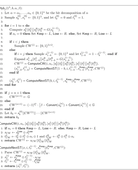
We proceed with a formal description of the optimized DPF construction, whose pseudocode is given in Figure 1.2
Theorem 3.3 (Optimized DPF). SupposeG:{0,1}λ→ {0,1}2(λ+1) is a pseudorandom
gen-erator. Then the scheme(Gen•,Eval•)from Figure 1 is a DPF for the family of point functions fα,β :{0,1}n →
G with key size n·(λ+ 2) +λ+dlog2|G|ebits. The number of PRG
invoca-tions in Gen is at most 2(n+dlog|G|
λ+2 e)and the number of PRG invocations in Evalis at most
n+dlog|G|
λ+2 e.
2A minor difference with respect to the conference version [10] is that the values oft(0) 0 , t
(0)
1 are fixed
Optimized Distributed Point Function
(
Gen
•,
Eval
•)
Let
G
:
{
0
,
1
}
λ→ {
0
,
1
}
2(λ+1)be a pseudorandom generator.
Let
Convert
G:
{
0
,
1
}
λ→
G
be a map converting a random
λ
-bit string to a pseudorandom group
element of
G
. (See Figure 3.)
Gen
•(1
λ, α, β,
G
):
1:
Let
α
=
α
1, . . . , α
n∈ {
0
,
1
}
nbe the bit decomposition of
α
2:
Sample random
s
(0)0← {
0
,
1
}
λand
s
(0)1
← {
0
,
1
}
λ 3:Let
t
(0)0= 0 and
t
(0)1= 1
4:
for
i
= 1 to
n
do
5:
s
L0||
t
L0s
R0||
t
R0←
G
(
s
(i−1)
0
) and
s
L1||
t
L1s
R1||
t
R1←
G
(
s
(i−1) 1
).
6:if
α
i= 0
then
Keep
←
L
,
Lose
←
R
7:
else
Keep
←
R
,
Lose
←
L
8:
end if
9:
s
CW←
s
Lose0⊕
s
Lose110:
t
LCW←
t
L0⊕
t
L1⊕
α
i⊕
1 and
t
RCW←
t
R0⊕
t
R1⊕
α
i 11:CW
(i)←
s
CW||
t
LCW||
t
RCW12:
s
(i)b←
s
Keepb⊕
t
(i−1)b·
s
CWfor
b
= 0
,
1
13:
t
(i)b←
t
Keepb⊕
t
(i−1)b·
t
KeepCWfor
b
= 0
,
1
14:
end for
15:
CW
(n+1)←
(
−
1)
t1n·
β
−
Convert
(
s
(n)0
) +
Convert
(
s
(n) 1)
∈
G
16:
Let
k
b=
s
(0)b
||
CW
(1)|| · · · ||
CW
(n+1) 17:return
(
k
0, k
1)
Eval
•(
b, k
b, x
):
1:
Parse
k
b=
s
(0)||
CW
(1)|| · · · ||
CW
(n+1), and let
t
(0)=
b
.
2:for
i
= 1 to
n
do
3:
Parse
CW
(i)=
s
CW||
t
LCW||
t
RCW 4:τ
(i)←
G
(
s
(i−1))
⊕
(
t
(i−1)·
s
CW||
t
LCW||
s
CW||
t
RCW)
5:
Parse
τ
(i)=
s
L||
t
Ls
R||
t
R∈ {
0
,
1
}
2(λ+1)6:
if
x
i= 0
then
s
(i)←
s
L, t
(i)←
t
L 7:else
s
(i)←
s
R,
t
(i)←
t
R8:
end if
9:
end for
10:
return
(
−
1)
b·
Convert
(
s
(n)) +
t
(n)·
CW
(n+1)∈
G
Figure 1: Pseudocode for optimized DPF construction for the class
f
α,β:
{
0
,
1
}
n→
G
. The symbol
Remark 3.4 (Early termination optimization). For the case of small output group G (e.g., G = Z2), we can further improve the complexity of (Gen•,Eval•) via an “early termination” optimization. Forν:= log2(λ/log2|G|), this optimization reduces the key size byν(λ+ 2) bits and the number of calls to the psuedorandom generator byν. See Section 3.2.3 for details.
Proof of Theorem 3.3. Correctness is argued similar to the tensor product case.
Security: We prove that each party’s key kb is pseudorandom. This will be done via a sequence of hybrids, where in each step we replace another correction wordCW(i) within the key from being honestly generated to being random.
The high-level argument for security will go as follows. Each party b∈ {0,1}begins with a random seeds(0)b that is completely unknown to the other party. In each level of key generation (fori = 1 to n), the parties apply a PRG to their seed s(bi−1) to generate 4 items: namely, 2 seeds sL
b, s R
b and 2 bits t L b, t
R
b. This process willalways be performed on a seed which appears
completely random and unknown given the view of the other party; because of this, the security of the PRG guarantees that the 4 resulting values appear similarly random and unknown given the view of the other party. The ith level correction word CW(i) will “use up” the secret randomness of 3 of these 4 pieces: the two bits tL
b, tRb, and the seed sLoseb for Lose ∈ {L, R}
corresponding to the directionexitingthe “special path”α: i.e.Lose=Lifα= 1 andLose=R
if α= 0. However, given this CW(i), the remaining seedsKeep
b for Keep 6= Lose still appears
random to the other party. The argument then continued in similar fashion to the next level, beginning with seedssKeepb .
For eachj∈ {0,1, . . . , n+ 1}, we will consider a distributionHybjdefined roughly as follows:
1. s(0)b ← {0,1}λ chosen at random (honestly), andt(0) b =b.
2. CW(1), . . . , CW(j)← {0,1}λ+1chosen at random.
3. Fori≤j,s(bi)||t(bi)computed honestly, as a function ofs(0)b ||t(0)b andCW(1), . . . , CW(j).
4. Forj, the other party’s seeds(1j−)b ← {0,1}λ is chosen at random, andt(j)
1−b= 1−t
(j)
b .
5. For i > j: the remaining values s(bi)||t(bi), s(1i−)b||t(1i−)b, CW(i) all computed honestly, as a function of the previously chosen values.
6. The output of the experiment iskb:=s(0)b ||CW(1)|| · · · ||CW(n+1).
Formally,Hybjis fully described in Figure 2. Note that whenj= 0, this experiment corresponds
to the honest key distribution, whereas whenj=n+ 1 this yields a completely random keykb.
We claim that each pair of adjacent hybrids j−1 andj will be indistinguishable based on the security of the pseudorandom generator.
The proof of Theorem 3.3 follows from the following four claims:
Claim 3.5. For every b∈ {0,1}, α∈ {0,1}n, β∈
G, it holds that
{kb←Hyb0(1
λ, b, α, β
)} ≡ {kb: (k0, k1)←Gen•(1λ, fα,β)}.
Claim 3.6. For every b∈ {0,1}, α∈ {0,1}n, β∈
G, it holds that
{kb←Hybn+1(1λ, b, α, β)} ≡ {kb←U}.
Note that Claims 3.5 and 3.6 follow directly by construction ofHybj.
Claim 3.7. There exists a polynomialp0 such that for any(T, PRG)-secure pseudorandom
gen-erator G, then for every j ∈[n], every b ∈ {0,1}, α ∈ {0,1}n, β ∈
G, and every nonuniform
adversaryArunning in time T0≤T−p0(λ), it holds that
Pr[kb←Hybj−1(1
λ, b, α, β);c
← A(1λ, kb) :c= 1]
−Pr[kb←Hybj(1
λ, b, α, β);c← A(1λ, k
b) :c= 1]
Hyb
j(1
λ, b, α, β
):
1:
Let
α
=
α
1, . . . , α
n∈ {
0
,
1
}
nbe the bit decomposition of
α
2:
Sample
s
(0)0, s
(0)1← {
0
,
1
}
λ, and let
t
(0)0
= 0 and
t
(0) 1= 1.
3:4:
for
i
= 1 to
n
do
5:
Compute
s
Lb
||
t
Lbs
Rb||
t
Rb=
G
(
s
(i−1) b
).
6:
if
α
i= 0
then
Set
Keep
←
L
,
Lose
←
R
.
else
, Set
Keep
←
R
,
Lose
←
L
7:8:
if
i < j
then
9:
Sample
CW
(i)← {
0
,
1
}
λ+2.
10:else
11:
if
i
=
j
then
Sample
s
1−b(j−1)← {
0
,
1
}
λand let
t
(j−1)1−b
= 1
−
t
(j−1)b
.
end if
12:Expand
s
L1−b||
t
L1−bs
R1−b||
t
R1−b=
G
(
s
(i−1) 1−b
).
13:CW
(i)=
ComputeCW
(
i, α
i,
[
s
L0||
t
L0s
R0||
t
R0]
,
[
s
L1||
t
L1s
R1||
t
R1]).
14:
(
s
(i)1−b, t
(i)1−b) =
ComputeNextST
(1
−
b, i, t
(i−1)1−b, s
Keep1−b||
t
Keep1−b, CW
(i))
15:
end if
16:
17:
(
s
(i)b, t
(i)b) =
ComputeNextST
(
b, i, t
(i−1)b, s
Keepb||
t
Keepb, CW
(i))
18:
end for
19:
20:
if
j
=
n
+ 1
then
21:
CW
(n+1)←
G
22:
else
23:
CW
(n+1)←
(
−
1)
t1n·
β
−
Convert
(
s
(n)0
) +
Convert
(
s
(n) 1)
∈
G
24:
end if
25:
Let
k
b=
s
(0)b||
CW
(1)|| · · · ||
CW
(n+1) 26:return
k
bComputeCW
(
i, α
i,
[
s
L0||
t
L0s
R0||
t
R0]
,
[
s
L1||
t
L1s
R1||
t
R1]):
1:
if
α
i= 0
then
Keep
←
L
,
Lose
←
R
.
else
,
Keep
←
R
,
Lose
←
L
2:s
CW←
s
Lose0⊕
s
Lose13:
t
LCW
←
t
L0⊕
t
L1⊕
α
i⊕
1 and
t
RCW←
t
R0⊕
t
R1⊕
α
i 4:return
CW
(i)←
s
CW||
t
LCW||
t
RCWComputeNextST
(
x, i, t
(i−1)x, s
Keepx||
t
Keepx, CW
(i)):
1:Parse
CW
(i)=
s
CW||
t
LCW||
t
RCW.
2:
s
(i)x←
s
Keepx⊕
t
(i−1) x·
s
CW 3:t
(i)x←
t
Keepx⊕
t
(i−1)x·
t
KeepCW4:
return
(
s
(i)x, t
(i)x).
Proof. Fix an arbitrary j ∈ [n], b ∈ {0,1}, α ∈ {0,1}n, β ∈
G. Given a Hyb-distinguishing adversary A with advantage for these values, we construct a corresponding PRG adversary B. Recall that in the PRG challenge for G, the adversary B is given a value r that is either computed by sampling a seed s ← {0,1}λ and computing r = G(s), or is sampled truly at
randomr← {0,1}2λ+2.
PRG adversaryB(1λ,(j, b, α, β), r):
1: Letα=α1, . . . , αn∈ {0,1}n be the bit decomposition ofα 2: Sample s(0)b ← {0,1}λ, and lett(0)
b =b.
3:
4: fori= 1 to (j−1)do
5: CW(i)← {0,1}λ+2. 6: ExpandsL
b||tLb
sRb||tRb =G(s (i−1)
b ).
7: ifαi= 0 thenSetKeep←L,Lose←R. else, SetKeep←R,Lose←L
8: (s(bi), t(bi)) =ComputeNextST(b, i, tb(i−1), sKeepb , tKeepb , CW(i)). 9: Taket(1i−)b= 1−t(bi).
10: end for
11:
12: Expand sL b||t
L b
sRb||tRb =G(s (i−1)
b ) and sets L
1−b||t L
1−b
sR1−b||tR1−b =r (the PRG challenge). 13: CW(j)=ComputeCW(j, αj,[sL0||tL0
sR0||tR0],[sL1||tL1
sR1||tR1]).
14: ifαj= 0 thenSetKeep←L,Lose←R. else, SetKeep←R,Lose←L
15: Compute (s(xj), t
(j)
x ) =ComputeNextST(x, j, t
(j−1)
x , sKeepx ||tKeepx , CW(j)), for bothx∈ {0,1}.
16:
17: Compute (CW(j+1)|| · · · ||CW(n+1)) =
RemainingKey(α, j, CW(1)|| · · · ||CW(j), t(0j), t(1j),[sL0||tL0
sR0||tR0],[sL1||tL1
sR1||tR1]). 18: returnkb=s(0)b ||CW(1)|| · · · ||CW(n+1).
RemainingKey(α, j, CW(1)|| · · · ||CW(j), t(j) 0 , t
(j) 1 ,[sL0||tL0
sR0||tR0],[sL1||tL1
sR1||tR1]): 1: fori= (j+ 1) to ndo
2: ExpandsL x||tLx
sRx||tRx =G(s (i−1)
x ) for bothx∈ {0,1}.
3: ifαi= 0 thenSetKeep←L,Lose←R. else, SetKeep←R,Lose←L
4: CW(i)=ComputeCW(i, αi,[sL0||tL0
sR0||tR0],[sL1||tL1
sR1||tR1]). 5: Compute (s(xi), t
(i)
x ) =ComputeNextST(x, i, t
(i−1)
x , sKeepx ||tKeepx , CW(i)), for bothx∈ {0,1}.
6: end for
7:
8: CW(n+1)←(−1)tn1 ·
β−Convert(s(0n)) +Convert(s(1n)) ∈G 9: return(CW(j)||CW(j+1)|| · · · ||CW(n+1))
Now, considerB’s success in the PRG challenge as a function of A’s success in distinguish-ing Hybj−1 from Hybj. If r is computed pseudorandomly, then it is clear the generated kb is
distributed asHybj−1(1λ, b, α, β).
It remains to show that ifrwas sampled at random then the generatedkb is distributed as Hybj(1λ, b, α, β). That is, ifris random, then the corresponding computed values ofs(j)
1−b and CW(j) are distributedrandomly conditioned on the values of s(0)
b ||t
(0)
b ||CW(1)|| · · · ||CW(j−1),
and the value oft(1j−)b is given by 1−t(bj). Note that all remaining values (for “level”i > j) are computed as a function of the values up to “level”j.
First, considerCW(j), computed in three parts:
• tL
CW =tLb ⊕tL1−b⊕αj.
In the case thatris random, thensLose
1−b, t L
1−b, andt R
1−b(no matter the value ofLose∈ {L, R}) are
each perfect one-time pads, and soCW(j)=sCW||tLCW||tRCW is indeed distributed uniformly. Now, condition on CW(j) as well, and consider the value ofs(j)
1−b. Depending on the value
oft(1j−−b1),s(1j−)b is selected either assKeep1−b orsKeep1−b ⊕sCW. However,sKeep1−b is distributed uniformly conditioned on the view thus far, and so in either case the resulting value is again distributed uniformly.
Finally, consider the value of t(1j−)b. Note that both tb(j) and t(1j−)b are computed as per
ComputeNextST, as a function oft(1j−1)andt(1j−−b1), respectively (andt(1j−−b1)was set to 1−t(bj−1)). In particular,
t(bj)⊕t(1j−)b= (tKeepb ⊕t(bi−1)·tCWKeep)⊕(tKeep1−b ⊕t1(i−−b1)·tKeepCW)
=tKeepb ⊕tKeep1−b ⊕(tb(i−1)⊕t(1i−−b1))·tKeepCW
=tKeepb ⊕tKeep1−b ⊕1·(tKeep0 ⊕tKeep1 ⊕1)
= 1
Combining these pieces, we have that in the case of a random PRG challenger, the resulting distribution of kb as generated by B is precisely distributed as is Hybj(1λ, b, α, β). Thus, the
advantage of B in the PRG challenge experiment is equivalent to the advantage of A in distinguishingHybj−1(1λ, b, α, β) fromHyb
j(1λ, b, α, β). The runtime ofBis equal to the runtime
ofAplus a fixed polynomialp0(λ). Thus for anyT0≤T−p0(λ), it must be that the distinguishing advantage ofAis bounded byPRG.
Claim 3.8. There exists a polynomial p0 such that for any (T, Convert)-secure pseudorandom
Convert : {0,1}λ →
G, then for every b ∈ {0,1}, α ∈ {0,1}n, β ∈ G, and every nonuniform
adversaryArunning in time T0≤T−p0(λ), it holds that
Pr[kb←Hybn(1
λ, b, α, β);c← A(1λ, kb) :c= 1]
−Pr[kb←Hybn+1(1λ, b, α, β);c← A(1λ, kb) :c= 1]
< Convert.
Proof. Fix an arbitrary b ∈ {0,1}, α ∈ {0,1}n, β ∈
G. In a similar fashion to the previous claim, an adversary A who distinguishes between the corresponding distributions Hybn and Hybn+1with advantagedirectly yields a corresponding adversaryBfor the pseudo-randomness of Convert with the same advantage, and only polynomial additional runtime p0(λ). Namely, B sampless(bn) ← {0,1}λ and all valuesCW(1), . . . , CW(n) ← {0,1}λ+2 at random, and then embeds theConvertchallenge by settingCW(n+1)= (−1)tn
1·[β+(−1)1−b·Convert(s(n)
b )+(−1) b·r].
In the case thatris generated pseudo-randomly as the output ofConvert(s(1n−)b) for randoms(1n−)b, this is precisely the distribution generated by Hybn. In the case that r is truly random, then it directly acts as a one-time pad on the remaining terms and thus CW(n+1) is distributed uniformly, precisely as perHybn+1. The claim follows.
This concludes the proof of Theorem 3.3.
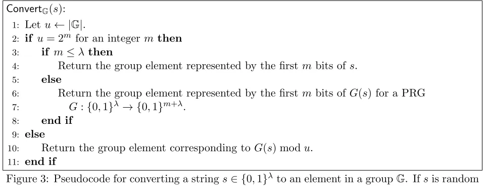
Convert
G(
s
):
1:
Let
u
← |
G
|
.
2:
if
u
= 2
mfor an integer
m
then
3:
if
m
≤
λ
then
4:
Return the group element represented by the first
m
bits of
s
.
5:
else
6:
Return the group element represented by the first
m
bits of
G
(
s
) for a PRG
7:
G
:
{
0
,
1
}
λ→ {
0
,
1
}
m+λ.
8:
end if
9:
else
10:
Return the group element corresponding to
G
(
s
) mod
u
.
11:
end if
Figure 3: Pseudocode for converting a string
s
∈ {
0
,
1
}
λto an element in a group
G
. If
s
is random
then
Convert
G(
s
) is pseudo-random.
Input
Output
Key length
Eval
•PRG
Eval
•AES
Gen
•PRG
Gen
•AES
Domain
Domain
in bits
operations
operations
operations
operations
{
0
,
1
}
nG
ν
(
λ
+ 2) + 2
λ
ν
ν
2
ν
4
ν
{
0
,
1
}
16{
0
,
1
}
1544
10
10
20
40
{
0
,
1
}
1272318
16
16
32
64
{
0
,
1
}
25{
0
,
1
}
2705
19
19
38
76
{
0
,
1
}
1273479
25
25
50
100
{
0
,
1
}
40{
0
,
1
}
4640
34
34
68
136
{
0
,
1
}
1275414
40
40
80
160
{
0
,
1
}
80{
0
,
1
}
9800
74
74
148
296
{
0
,
1
}
12710574
80
80
160
320
{
0
,
1
}
160{
0
,
1
}
20120
154
154
308
612
{
0
,
1
}
12720894
160
160
320
640
Table 1: Performance of the optimized DPF construction from Figure 1. We use the additional
early termination
optimization, which ends the path that
Gen
•and
Eval
•follow at level
ν
=
min
{d
n
−
log
logλ|G|
e
, n
}
of the tree. With this optimization, the key length is
ν
(
λ
+ 2) + 2
λ
. The
PRG
G
expanding
s
∈ {
0
,
1
}
127to 256 bits can be implemented either by AES in counter mode,
i.e.
G
(
s
) = AES
s||0(0)
||
AES
s||0(1) or by the fixed-key implementation proposal of [38] using the
compression function of [32], i.e.
G
(
s
) = (AES
k0(
s
||
0)
⊕
s
||
0)
||
(AES
k1(
s
||
0)
⊕
s
||
0) for two fixed
keys
k
0, k
1. In either case,
Gen
•requires two AES operations per PRG expansion since it uses the
3.2.3
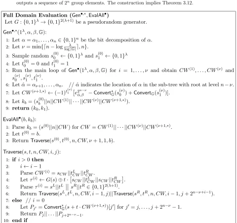
Full Domain Evaluation
Some applications of DPF require running the evaluation algorithmEval• on every element of the input domain. This is the case, for instance, for the application to 2-server PIR described in the Introduction, or “writing” applications such as the private updates application described in Appendix A (see also [34]). For input domain of sizeN = 2n, a straightforward implementation
usesN independent invocations ofEval•, once for each input. In this section we present a more efficient scheme that uses the tree structure of our DPF to reduce the total cost by roughly a factor ofn.
Notation 3.10. LetGbe a group,β ∈Gand letj, ibe two integers such that 0≤j < i. For any sequencea∈Giwe denote bya[j] thej-th element in the sequence. We denote byei
j,β∈Gi
the sequence ofi group elements such that ei
j,β[j] =β and e i j,β[j
0] is the unit element for any
j06=j. Ifi= 1 thenei
j,β is simplyβ. For any two sequencesγ0, γ1∈Gi letγ0+γ1∈Gi denote the component-wise addition of elements over the group.
Definition 3.11. In the same setting as Definition 2.2 we say that a protocol (Gen,EvalAll) is a full domain evaluation protocol forF if the secrecy property is identical to Definition 2.2 and
• Correctness: For all ˆf ∈ PF describing f : {0,1}n → G, and every x ∈ {0,1}n, if (k1, . . . , km)←Gen(1λ,fˆ) then∀iEvalAll(i, ki)∈G2
n
and
Pr "m
X
i=1
EvalAll(i, ki)[x] =f(x) #
= 1.
Similarly to Definition 2.2 for m = 2 we define a subtractive full domain evaluation pro-tocol in the same way as above, except that m ranges over 0 and 1 and EvalAll(0, k0)[x]− EvalAll(1, k1)[x] =f(x).
We present a protocol (Gen•,∗,EvalAll•) for full domain evaluation of a two-party DPF, improving on the computational complexity of the na¨ıve solution by a factor of O(n). We leverage the structure of our particular DPF scheme to optimize the construction in two ways. Consider a rooted binary tree whose leaves are the inputsx∈ {0,1}n and the path from the
root to a leaf xreflects the binary representation x. More concretely, ifxi= 0 (resp.,xi= 1), then thei-th step in the path moves from the current node to its left (resp., right) child. In our DPF construction, a single invocation ofEval•(b, kb, x) traverses the path from the root to a leaf
x, and so the na¨ıve algorithm for full domain evaluation traverses each of these paths, requiring a total ofO(nN) invocations of the PRG. The first improvement is based on the observation that for every nodeiin the tree there is a uniqueτ(i)value computed by any execution ofEval• that traverses the node. Since the τ values and the correction words are sufficient to compute the output of Eval• on every single input, full domain evaluation can be carried out by computing theτ values for each node in the tree, requiring onlyO(N) PRG invocations.
A second improvement is the early termination optimization for small output groups. The correction wordCW(n+1) inGen• is the outputβ masked by the expansion of two seeds. If the representation ofβ is short then several output values can be “packed” intoCW(n+1). For any nodeV of depthν in the tree there are 2n−ν leaves in its sub-tree, or 2n−ν input elements with
a shared prefix that ends atV. If the size ofCW(ν+1)is at least 2n−ν times the output length
then the main loop of bothGen• andEval•can terminate at levelνinstead of at leveln. In this caseCW(ν+1) will be a sequence of group elements masked by the two expanded seeds. The sequence will have the outputβ in the location specified by the lastn−νbits ofαand the unit element ofGin every other location.
Convert is that in Line 4 Convert∗ returns bλ/mc group elements defined by the first bλ/mc blocks ofmbits ins.
The pseudo-code in Figure 4 describes Gen•,∗ and EvalAll•. Gen•,∗ makes the necessary adjustments toGen• enabling early termination. EvalAll• performs full domain evaluation and outputs a sequence of 2n group elements. The construction implies Theorem 3.12.
Full Domain Evaluation (
Gen
•,∗,
EvalAll
•)
Let
G
:
{
0
,
1
}
λ→ {
0
,
1
}
2(λ+1)be a pseudorandom generator.
Gen
•,∗(1
λ, α, β,
G
):
1:
Let
α
=
α
1, . . . , α
n∈ {
0
,
1
}
nbe the bit decomposition of
α
.
2:Let
ν
= min
{d
n
−
log
logλ|G|
e
, n
}
.
3:Sample random
s
(0)0← {
0
,
1
}
λand
s
(0)1
← {
0
,
1
}
λ 4:Let
t
(0)0= 0 and
t
(0)1= 1
5:
Run the main loop of
Gen
•(1
λ, α, β,
G
) for
i
= 1
, . . . , ν
and obtain
CW
(1), . . . , CW
(ν)and
s
(ν)0, s
(ν)1, t
(ν)1.
6:
Let ˆ
α
=
α
ν+1, . . . , α
n.
// ˆ
α
indicates the location of
α
in the sub-tree with root at level
n
−
ν
.
7:
Let
CW
(ν+1,∗)←
(
−
1)
t(1ν)e
2 n−νˆ
α,β
−
Convert
∗ G(
s
(ν)
0
) +
Convert
G(
s
(ν) 1)].
8:
Let
k
b= (
s
(0)b
||
n
||
CW
(1)|| · · · ||
CW
(ν)||
CW
(ν+1,∗)
).
9:
return
(
k
0, k
1).
EvalAll
•(
b, k
b):
1:
Parse
k
b= (
s
(0)||
n
||
CW
) for
CW
=
CW
(1)|| · · · ||
CW
(ν)||
CW
(ν+1,∗).
2:Let
t
(0)=
b
.
3:
Return
Traverse
(
s
(0), t
(0), n, CW, ν
+ 1
,
1
, b
).
Traverse
(
s, t, n, CW, i, j
):
1:
if
i >
0
then
2:
i
←
i
−
1
3:
Parse
CW
(i)=
s
CW||
t
LCW||
t
RCW.
4:Let
τ
(i)←
G
(
s
)
⊕
t
·
s
CW||
t
LCW||
s
CW||
t
RCW.
5:
Parse
τ
(i)=
s
L||
t
Ls
R||
t
R∈ {
0
,
1
}
2(λ+1).
6:
Return
Traverse
(
s
L, t
L, n, CW, i
−
1
, j
)
||
Traverse
(
s
R, t
R, n, CW, i
−
1
, j
+ 2
n−ν+i−1).
7:
else
//
i
= 0
8:
Let
P
j0=
Convert
∗G
(
s
+
t
·
CW
(ν+1,∗)
)[
j
0] for
j
0=
j, . . . , j
+ 2
n−ν−
1.
9:Return
P
j||
. . .
||
P
j+2n−ν−1.
10:
end if
Figure 4: Pseudocode for optimized DPF evaluation on the entire input domain.
Theorem 3.12 (Full domain evaluation). Let λ be a security parameter, let G : {0,1}λ →
{0,1}2(λ+1) be a PRG and let
Gbe a group. The scheme(Gen•,∗,EvalAll•)in Figure 4 is a full
domain evaluation protocol for the family of point functions from {0,1}n to
G. The keys that Gen•,∗outputs are of size at mostν(λ+ 2) +λ+ logn+ max{λ,log|G|}bits, the number of PRG
invocations inGen•,∗ is at most2ν+ 2dlog|G|
λ+2 eand the number of PRG invocations in EvalAll •
is at most2ν(1 +dlog|G|
λ+2 e)forν = min{dn−log
λ
Proof. The security of the protocol follows immediately from the security of the protocol in Figure 1 since the keys produced by Gen•,∗(1λ, α, β,
G) are identical to the keys generated by Gen•(1λ,(α
1, . . . , αν), e2
n−ν
ˆ
α,β ,G2 n−ν
), where (α1, . . . , αν) is theν-bit prefix ofα.
To prove the correctness of the protocol we observe that for every x∈ {0,1}n, everyi < ν
and any b, the value τ(i) that EvalAll•(b, kb) generates for the tree node associated with the
i-bit prefix of xis identical to the τ(i) value that Eval•(b, kb, x) produces. For any 1 ≤i < ν and any xthat does not have a shared i-bit prefix withα, the invocationsEval•(0, k0, x) and Eval•(1, k1, x) produce the same valuesτ(j)for anyi≤j≤ν. Therefore
EvalAll•(0, k0)[x]−EvalAll•(1, k1)[x] = 0.
If x shares a prefix of length ν with α then the choice of CWν+1,∗ and the fact that t(ν) 0 ⊕
t(1ν)= 1 ensure thatEvalAll•(0, k0)[x]−EvalAll•(1, k1)[x] = 0 forx6=αandEvalAll•(0, k0)[α]− EvalAll•(1, k1)[α] =β.
Each key kb includes the values s
(0)
b and nwhich are of length λ+ logn together and the ν + 1 strings CW(1), . . . , CW(ν), CW(ν+1,∗). CW(i) is of length λ+ 2 for i = 1, . . . , ν and the length CW(ν+1,∗) is |CW(ν+1,∗)| = max{λ,log|
G|}. Therefore, the key size is at most
ν(λ+ 2) +λ+ logn+ max{λ,log|G|}.
Gen•,∗executes the PRGGtwice for eachi= 1, . . . , νexpanding the seedss(i−1) 0 , s
(i−1) 1 and runs twoConvertoperations ons(0ν), s1(ν), which is together 2ν+ 2dlog|G|
λ+2 ePRG operations. The tree thatEvalAll•traverses has 2νleaves and 2ν−1 internal nodes. There is one PRG operation
per internal node and at mostdlog|G|
λ+2 eoperations per each leaf, which completes the proof.
Remark 3.13. In the useful case of|G|= 2k elements fork≤λ, Theorem 3.12 overestimates the number of PRG invocations inEvalAll•by a factor of two sinceConvertG(s) for each element in level ν of the tree does not require additional PRG operations. For the same reason, in this case the number of PRG operations in Gen•,∗ is exactly 2ν and the key size is at most
ν(λ+ 2) + 2λ+ logn.
3.3
FSS for Decision Trees
We now describe how the tensoring approach can be utilized to provide FSS for the broader class of decision trees. A decision tree is defined by: (1) a tree topology, (2) variable labels on each node v (where the set of possible values of each variable is known; we denote this set for the variable of nodev bySv), (3) value labels on each edge (the possible values from Sv), and (4) output labels on each leaf node.
In our construction, the key size is roughly λ· |V| bits, where V is the set of nodes, and evaluation on a given input requires|V|executions of a pseudorandom generator, and a compa-rable number of additions. The FSS is guaranteed to hide the secret edge value labels and leaf output labels (which we refer to as “Decisions”), but (in order to achieve this efficiency) reveals the base tree topology and the identity of which variable is associated to each node (we refer to this collective revealed information as “Tree”).
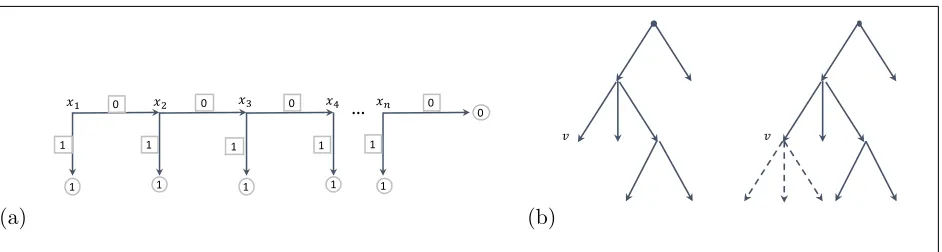
As a simple illustrative example, consider a decision tree representation of the OR function onn bits xi. The tree topology includes a length-nchain of nodes (each labeled by a unique
input variablexi), with edges all labeled by 0, ending in a terminal output node (labeled by 0).