Monash University Wellington Road CLAYTON Vic 3168 AUSTRALIA Telephone:
(03) 990 52398, (03) 990 55112 from overseas:
61 3 990 55112
Fax numbers: from overseas:
(03) 990 52426, (03)990 55486 61 3 990 52426 or 61 3 990 55486
e-mail [email protected]
Structural Change, the Demand
for Skilled Labour and Lifelong
Learning
G. A. Meagher
Centre of Policy Studies
Monash University
General Paper No. G-121 August 1997
ISSN 1 031 9034 ISBN 0 7326 0742 6
The Centre of Policy Studies (COPS) is a research centre at Monash University devoted to quantitative analysis of issues relevant to Australian economic policy. The Impact Project is a cooperative venture between the Australian Federal Government, Monash University and La Trobe University. COPS and Impact are operating as a single unit at Monash University with the task of constructing a new economy-wide policy model to be known as MONASH. This initiative is supported by the Industry Commission on behalf of the Commonwealth Government, and by several other sponsors. The views expressed herein do not necessarily represent those of any sponsor or government.
C
ENTRE
of
P
OLICY
S
TUDIES
and
the
I
MPACT
i
In a recent report, the Organisation for Economic Cooperation and Development has argued that certain key developments, including globalisation, population ageing and the diffusion of information technologies, are causing a shift in the demand for labour in modern advanced economies. Demand is thought to be moving away from relatively low-skilled agricultural and production occupations in favour of highly-skilled professional, technical, administrative and managerial occupations. Moreover, rising turnover in the labour market is tending to increase the rate at which existing skills are rendered obsolete. Hence workers in OECD countries are coming under mounting pressure to adapt and enhance their skills on an ongoing basis; that is, today's workers must participate in lifelong learning.
This paper investigates the quantitative evidence for the proposition using, as a case study, the distribution of employment across occupations in Australia. Three changes in this distribution are considered: the change that actually occurred between 1986-87 and 1994-95, a forecast of the change that is likely to occur between 1994-95 and 2002-03, and an estimate of the change that will result from trade liberalisation proposals advanced by the Asia Pacific Economic Cooperation forum. In each case the change in the occupational distribution is used to infer the effect on the demand for labour differentiated by qualification level, qualification field and age group. Unlike much of the structural analysis that accompanies discussions of lifelong learning, the approach here is comprehensive. The analysis is not restricted to occupations thought on a priori grounds to have a particular affinity to lifelong learning, but considers changes in employment across all occupations. Hence the role of particular occupations, such as those associated with information technology, for example, are able to be placed in a an economy-wide perspective.
The analysis reveals that the factors driving the demand for labour are numerous and diverse, and suggests that generalisations and "stylised facts" are likely to be of only limited usefulness in determining training priorities.
iii
1 Introduction 1
2 Methodology 3
2.1 The Historical Simulation 3
2.2 The Forecast Simulation 4
2.3 The APEC Simulation 6
3 Results 8
3.1 Employment by Qualification Level 8
3.1.1 Bachelor degree 10 3.1.2 Skilled vocational 16 3.1.3 No post-school qualification 18
3.2 Employment by Qualification Field 18
3.3 Employment by Age Group 20
3.4 APEC Simulation 22
4 Concluding Remarks 25
iv
1 Employment Changes by Qualification Level 9
2 Employment Shares by Qualification Level 9
3 Employment Changes by Qualification Level
and Occupation, Historical Simulation 11
4 Employment Changes by Qualification Level
and Occupation, Forecast Simulation 13
5 Employment Changes by Qualification Field 19
6 Employment Changes by Age Group 21
7 Employment Changes by Age Group and
Qualification Field, Forecast Simulation
by
G.A.Meagher
Centre of Policy Studies, Monash University, Australia
1. Introduction
In January 1996, the Education Committee of the Organisation for Economic Cooperation and Development (OECD) met at Ministerial Level to consider the theme "Making Lifelong Learning a Reality for All". Subsequent to the meeting, the OECD published a background report (OECD, 1996) providing detailed information on all the topics discussed by the Ministers. One function of the report was to establish the context for lifelong learning through an analysis of a wide range of social, economic and educational data. In this regard, the report argues
"the ideas that underpin the broad principle (of lifelong learning) need to be grounded in an analysis of key facts and developments, and not merely founded on an assertion of anticipated benefits." (p. 29)
The purpose of this paper is to investigate some of these ideas in more quantitative detail than that attempted by the OECD, using the Australian economy as a case study. As a small, open, developed economy, Australia has been subject in recent times to all the key developmental pressures mentioned above and, to that extent, its experience can be considered of general relevance to OECD countries. Indeed, local commentators on lifelong learning have raised the same kind of considerations as the OECD in the Australian context. For example, in a review of pressures on Australian university graduates to continue learning after graduation, Candy et al. (1994) nominate the following trends as being of particular significance: occupational mobility and the emergence of new occupations, the explosion of knowledge and technology, the shift to an information society, increasing internationalisation and microeconomic reform.
In the same vein, Clare and Johnson (1993) offer this assessment of the imperative for ongoing education:
"In many vocational areas, techniques and skills are constantly evolving. Keeping skills up to date is necessary for Australia to maintain or enhance levels of competitiveness, and to supply the quality of goods and services that is increasingly being expected. In addition, Australia's population is ageing, and the proportion of young people in work is declining. The trend towards an older population will effect the overall levels of knowledge that are held by the workforce. All knowledge suffers from some level of depreciation or obsolescence, and depreciation rates for knowledge have increased as technology changes many facets of the work we perform. Therefore the stock of knowledge in the workforce will decline unless more knowledge is gained by existing workers, through experience and training, to counteract the effects of knowledge depreciation." (p.48)
The focus of the present analysis of the quantitative evidence is the distribution of employment across occupations. Three changes in this distribution are considered: the change that actually occurred between 1986-87 and 1994-95 (which shall be referred to as the historical simulation), a forecast of the change that is likely to occur between 1994-95 and 2002-03 (the forecast simulation), and an estimate of the change that will result from trade liberalisation proposals advanced by the Asia Pacific Economic Cooperation forum (the APEC
simulation). In each case the change in the occupational distribution is used to
qualification field and age group. In order to facilitate a comparison of the three simulations, the analysis abstracts from the role of the business cycle in determining the level of employment; that is, the analysis is concerned with the effects of structural change as embodied in changes in the distribution of employment. Unlike much of the structural analysis that accompanies discussions of lifelong learning, the approach here is comprehensive. The analysis is not restricted to occupations thought on a priori grounds to have a particular affinity to lifelong learning, but considers changes in employment across all occupations. Hence the role of particular occupations, such as those associated with information technology, for example, are able to be placed in a an economy-wide perspective.
In the balance of the paper, methodological details are provided in Section 2, results are presented in Section 3 and conclusions are drawn in Section 4.
2. Methodology
The simulations begin with a (282 x 330) matrix of employment by occupation and qualification taken from the 1991 Census of Population and Housing. 1991 is the most recent year for which the required data is available.1 The 282 occupations comprise the unit groups of the Australian Standard Classification of Occupations (ASCO) and are described in the ASCO Dictionary published by the Australian Bureau of Statistics (ABS, 1987). All but one of the 330 qualification categories are obtained by dividing each of 47 qualification fields between 7 qualification levels. The qualification levels and fields are described below in Tabes 1 and 3, respectively. The remaining category, namely No
post-school qualification, is included for the sake of completeness. This matrix, i.e.,
the matrix of actual employment levels in 1991, will be referred to as the base
matrix. Its main function is to define the distribution of qualifications within
each occupation.
2.1 The Historical Simulation
The historical simulation is based on quarterly employment data for the ASCO unit groups taken from the ABS Labour Force Survey and covers the period
1 A more recent census was conducted by the Australian Bureau of Statistics in 1996 but processing of
August 1986 to May 1995. After first converting the data into four-quarter moving averages, ordinary least squares regression is used to determine the trend change in employment for each occupation between 1986-87 and 1994-95.
Given the qualification distributions defined by the base matrix, it would be possible to compute the corresponding changes in employment by qualification immediately. However, in order to compare the effects of the historical changes with those of the forecast and APEC simulations, the occupational employment changes must be imposed on a common base. Moreover, for purposes of the present study, interest is focussed on the effects of changes in the distribution, rather than the level, of employment. Hence the historical
matrix is computed by first scaling each row of the base matrix separately to
conform to the trend occupational changes (i.e., the historical employment changes are imposed on the 1991 employment levels) and then scaling the entire matrix to recover the 1991 level of aggregate employment.
The historical simulation is completed by comparing the column sums of the historical and base matrices. The differences between the column sums represent the changes in employment by qualification that can be attributed to the change in the distribution of employment across occupations between 1986-87 and 1994-95.2
2.2 The Forecast Simulation
The forecast simulation proceeds in four stages. It begins with a forecast for the macroeconomy derived from the views of two of Australia's leading commercial forecasting agencies, Syntec Economic Services and Access Economics.3 This forecast identifies, inter alia, the prospects for Gross Domestic Product (GDP) and its components (i.e., investment, private consumption, government expenditure, exports and imports), and for aggregate employment, over the forecast period 1994-95 to 2002-03.
2 Of course, the results are conditional on the particular qualification distributions embodied in the base
matrix. However, these distributions vary sufficiently across occupations to suggest that the important structural characteristics of the matrix persist over the time periods in question.
3 Both organisations regularly publish medium-term macro forecasts for the Australian economy. The
At the second stage, the aggregate forecasts are converted into forecasts of output and employment for 112 industries.4 This conversion is achieved by treating the macro forecast as an exogenous input to a large, dynamic, applied general equilibrium model of the Australian economy, the MONASH model. Additional informed opinion about the outlook for particular industries is also included at this stage. For example, although Australia is a developed economy, its overall economic prospects continue to depend to a significant extent on its export-oriented primary sector. Hence, a considerable effort is made by the Australian Bureau of Agricultural and Resource Economics to anticipate developments in the relevant world commodity markets. The Bureau's assessments are published on an annual basis5 and are incorporated into the present forecasts.
Of particular importance among the range of informed opinion is a view about future technical change. Technical change cannot be observed directly but must be inferred from movements in other variables. In an independent study, the MONASH model has been used to estimate the technical change that must have occurred in the Australian economy during the period 1986-87 to 1993-94 to support consistency between a wide variety of observations including6
• outputs for 90 industries,
• employment for 80 industries,
• capital growth for 30 industries,
• investment for 25 industries,
• import and export volumes and prices for 114 commodities,
• value-added prices for 17 industries,
• consumer prices for 26 commodities,
• consumption volumes for 38 commodities,
• tariff rates for 114 commodities, and
• public expenditures for 114 commodities.
This study informs the forward estimates of technical change at the industry level, such as intermediate-input-saving technical change and
4 In the forecast scenario, labour is assumed to be in excess supply so that employment is demand
determined. In other words, references to employment forecasts should, strictly speaking, be taken to mean forecasts of the demand for labour.
5 See Australian Bureau of Agricultural and Resource Economics (1996).
6 The MONASH model identifies 112 industries which produce 114 commodities. The numbers of
saving technical change. By and large, the rate of technical change that has obtained in the recent past is assumed to continue in the forecast period, although a limited number of adjustments have been made on the basis of anecdotal information. The methodology employed in the historical study is described in Dixon and McDonald (1993) and Dixon et al. (1996).
At the third stage of the forecast simulation, the 112 industry employment forecasts are converted into employment forecasts for 282 occupations. Changes in the distribution of employment across occupations within an industry are treated as a type of technical change. To estimate this type of change, a quarterly time series was assembled for each industry showing the 282 occupational employment shares between August 1986 and May 1995, inclusive.7 This data was derived from the ABS Labour Force Survey and from the 1986 and 1991 Censuses of Population and Housing. Simple linear time trends in the occupational shares were then determined using ordinary least squares regression. The occupational forecasts are obtained by extrapolating these trends into the forecast period.
The final stage consists of computing the forecast matrix in a manner analogous to the computation of the historical matrix; that is, the changes in employment by occupation over the forecast period are imposed on the rows of the base matrix and the resulting matrix is scaled to recover the 1991 level of aggregate employment.
The MONASH forecasting system that underlies the forecast simulation has been under development at the Centre of Policy Studies at Monash University since 1991 and is documented in Adams et al. (1994). The particular set of forecasts presented here is a slightly revised version of the set described in Dixon and Rimmer (1996).
2.3 The APEC Simulation
In the Bogor Declaration of November 1994, the member countries of the Asia Pacific Economic Cooperation (APEC) forum8 committed themselves to free
7 Data availability meant that the estimation was conducted for an 88-industry classification rather than
the full 112-industry classification of the MONASH model. Details of the estimation procedure are contained in Meagher (1997).
8 The APEC members are Canada, the United States, Mexico, New Zealand, Australia, the five ASEAN
and open trade within the group by the year 2020. Adams et al. (1996) have recently conducted an analysis of the consequences for Australia of such a change in trading relations using the GTAP model of world trade (Hertel, 1997).9 In particular, the GTAP model is used to calculate how production levels, bilateral trade flows and prices of thirty seven commodities are affected when all tariffs (and the tariff equivalents of other trade barriers) on APEC sourced imports are removed by each APEC country. The GTAP results are then treated as exogenous inputs to a complementary simulation using the
MONASH model. In this arrangement, the function of GTAP is to determine
the effect of the introduction of trade liberalisation on the supply curves facing Australia's importers and the demand curves facing its exporters, while the function of MONASH is to determine the effect of the changes in foreign demands and supplies on the employment of labour by industry and occupation. In the present context, the changes in employment by occupation are used to compute the APEC matrix, i.e., the employment matrix obtained by imposing the changes on the rows of the base matrix and then scaling the resulting matrix to recover the 1991 level of aggregate employment. As with the other simulations, the end product of the APEC simulation is obtained by computing the difference between the column sums of the APEC matrix and the column sums of the base matrix.
In the historical and forecast simulations, the structural change considered represents differences between the state of the economy at two different points in time. In the APEC simulation, it represents differences between two alternative states of the economy at the same point of time. The two alternatives are the state that will evolve if the trade liberalisation is actually implemented and the state that will evolve if it is not. If the reform were to occur now, it would take the economy a number of years to adjust to the change (i.e., to return to equilibrium), exactly how long depending on the kind of adjustment mechanisms that are allowed in the simulation (i.e., on the closure of the model). Adams et al. report results for a medium-run closure and a long-run closure. In the former, the size of the capital stock and the labour force in each GTAP region10 are treated as being unaffected by the reform. Thus the medium run is a period of time long enough to allow the reorganisation of production and distribution within the regional economies but not long enough
9 The GTAP model is maned after the Global Trade Analysis Project located at Purdue University in
the United States.
to allow the sizes of the regional economies to change (that is, to diverge from the sizes they would have assumed in the absence of the reform). In the long-run closure, these restrictions are relaxed to the extent that the global quantity of capital and its regional distribution are allowed to respond to the changed profit opportunities created by APEC. It is in the nature of the kind of comparative static analysis involved here that the elapsed calender times during the medium and long runs are not explicitly stated. However, Adams et al. believe that periods of about 5 to 7 years and about 15 to 20 years, respectively, may be appropriate. In this paper, APEC results are reported only for the medium run, as it represents an adjustment period that corresponds more closely to the other two simulations.
3. Results
3.1 Employment by Qualification Level
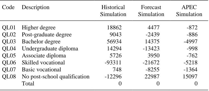
Table 1. Employment Changes by Qualification Level, Persons
Code Description Historical Forecast APEC Simulation Simulation Simulation QL01 Higher degree 18862 4477 -872 QL02 Post-graduate degree 9043 -2439 -886 QL03 Bachelor degree 56934 14375 -4997 QL04 Undergraduate diploma 14294 -13423 -998 QL05 Associate diploma 5726 3950 -762 QL06 Skilled vocational -93311 -21672 -5218 QL07 Basic vocational 748 -8255 -1364 QL08 No post-school qualification -12296 22987 15097
Total 0 0 0
A different appreciation of the relationship between the simulations emerges in Table 2, where the results are expressed as percentages of total employment. According to this table, the actual distribution of employment in 1991 is no more than mildly disrupted by any of the three simulations, with no category changing its employment share by more than one and a half percentage points. Hence the dissimilarities between the columns of results in Table 1 are more apparent than substantive, and arise primarily because each column represents the difference between two (not particularly dissimilar) distributions.
Table 2. Employment Shares by Qualification Level, Per Cent
Code Description Actual Historical Forecast APEC 1990-91 Simulatio
n
Simulatio n
Simulatio n QL01 Higher degree 1.71 1.97 1.77 1.70 QL02 Post-graduate degree 1.68 1.81 1.65 1.67 QL03 Bachelor degree 9.89 10.69 10.10 9.82 QL04 Undergraduate diploma 6.21 6.41 6.02 6.19 QL05 Associate diploma 2.40 2.48 2.46 2.39 QL06 Skilled vocational 16.64 15.33 16.34 16.57 QL07 Basic vocational 7.20 7.22 7.09 7.19 QL08 No post-school
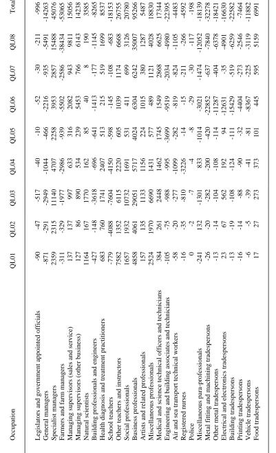
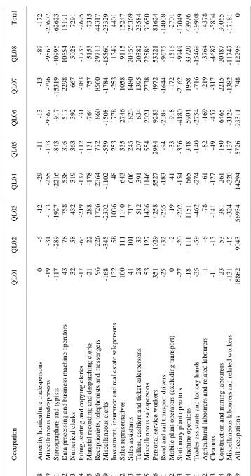
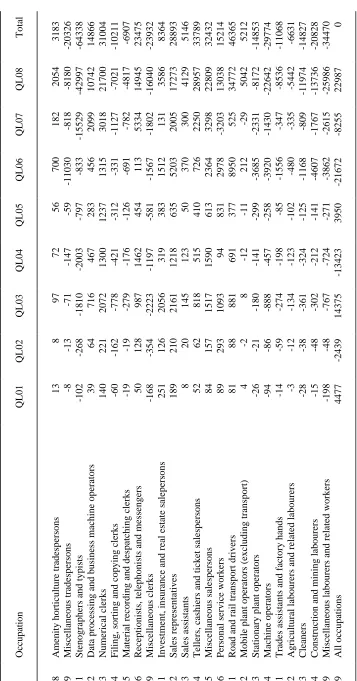
The economic forces driving the results in Table 1 can be better understood by identifying separately the contributions which various occupations make to changes in employment by qualification level. Table 3 shows the relevant occupation by qualification matrix for the historical simulation11, the entries in the last row (i.e., the column sums) of the table corresponding to the entries in the first column of Table 1. Table 4 contains the analogous information for the forecast simulation. Two general observations are again pertinent. Firstly, persons with qualifications of a particular level are distributed across numerous occupations. Secondly, the changes in the distribution of employment across occupations in the two simulations are quite diverse. Together, these two observations imply that the effect of structural change on the skill composition of employment cannot to be satisfactorily explained by reference to "stylised facts", intuitively appealing though they may be. Rather, because it is multi-layered, the relationship between cause and effect tends to be quite opaque and, in general, can only be revealed by means of a somewhat tedious multi-step analysis. Three examples will be provided.
3.1.1 QL03 Bachelor degree
Both the historical and the forecast simulations favour the employment of persons with bachelor degrees, but the former does so much more than the latter. From Table 1, the difference is (56934-14375) or 42559 persons. From Tables 3 and 4, this difference is mainly accounted for by the occupations
• 27 Business professionals (29051-17145=11906 persons),
• 23 Health diagnosis and treatment practitioners (9445),
• 26 Social professionals (6504) and
• 24 School teachers (6090).
All the remaining occupations account for 8614 persons.
Employment growth for a particular occupation can be usefully decomposed into a component (the industry growth effect) due to industry employment growth and a component (the occupational share effect) due to changes in the distribution of employment across occupations within industries. In the case of
Business professionals, the difference between the historical and forecast
employment growth rates reflects almost entirely a difference in the
Table 3: Employment Changes by Qualification Level
(a)
and Occupation, Historical Simulation, Persons
Occupation QL01 QL02 QL03 QL04 QL05 QL06 QL07 QL08 11
Legislators and government appointed officials
-90 -47 -517 -40 -10 -52 -30 -211 12 General managers -871 -291 -2949 -1044 -466 -2216 -935 -5491 13 Specialist managers 2359 2315 11140 4707 2258 3953 2857 15488 14
Farmers and farm managers
-311 -329 -1977 -2986 -939 -5502 -2586 -38434 15
Managing supervisors (sales and service)
137 137 997 633 316 2082 943 9811 16
Managing supervisors (other business)
127 86 890 534 239 5453 766 6143 21 Natural scientists 1164 167 1770 162 85 40 8 190 22
Building professionals and engineers
-427 -148 -3618 -696 -641 -1413 -177 -1145 23
Health diagnosis and treatment practitioners
683 760 1741 2407 513 215 519 1699 24 School teachers -779 -4088 -7604 -4150 -598 -145 -108 -683 25
Other teachers and instructors
7582 1352 6115 2220 605 1039 1174 6668 26 Social professionals 1657 1932 10732 1691 531 411 699 3126 27 Business professionals 4858 4061 29051 5717 4024 6304 6242 35007 28
Artists and related professionals
157 135 1133 1156 224 1015 380 1287 29 Miscellaneous professionals 2524 1970 6690 1431 577 489 1121 4028 31
Medical and science technical officers and technicians
384 261 2448 1462 1745 1549 2868 6625 32
Engineering and building associates and technicians
-105 -75 -988 -995 -3699 -9519 -2034 -4980 33
Air and sea transport technical workers
-58 -20 -277 -1099 -282 -819 -824 -1105 34 Registered nurses -16 -35 -810 -3226 -14 -15 -211 -266 35 Police 0 -2 -7 -4 -8 -29 -30 -117 39 Miscellaneous para-professionals -241 132 -1301 833 -1014 -3021 -1474 -12052 41
Metal fitting and machining tradespersons
-26 -20 -282 -200 -420 -22852 -637 -7840 42
Other metal tradespersons
-13 -14 -104 -108 -114 -11287 -404 -6378 43
Electrical and electronics tradespersons
Table 3 (continued): Employment Changes by Qualification Level
(a)
and Occupation, Historical Simulation, Persons
Occupation QL01 QL02 QL03 QL04 QL05 QL06 QL07 QL08 48
Amenity horticulture tradespersons
0 -6 -12 -29 -11 -13 -13 -89 49 Miscellaneous tradespersons -19 -31 -173 -255 -103 -9367 -796 -9863 51
Stenographers and typists
-117 -289 -1927 -2216 -843 -917 -15319 -40996 52
Data processing and business machine operators
43 78 758 538 305 517 2298 10654 53 Numerical clerks 32 58 432 319 363 392 667 5028 54
Filing, sorting and copying clerks
-17 -63 -219 -137 -112 -31 -383 -1733 55
Material recording and despatching clerks
-21 -22 -288 -178 -131 -764 -757 -5153 56
Receptionists, telephonists and messengers
96 226 1726 2364 772 860 8560 29713 59 Miscellaneous clerks -168 -345 -2302 -1102 -559 -1508 -1784 -15560 61
Investment, insurance and real estate salepersons
132 58 1036 48 253 1778 -253 1349 62 Sales representatives 100 111 1140 643 335 2746 1058 9115 63 Sales assistants 41 101 717 606 245 1823 1480 20356 64
Tellers, cashiers and ticket salespersons
28 33 512 391 207 634 1395 20382 65 Miscellaneous salespersons 53 127 1426 1146 554 2021 2738 22586 66
Personal service workers
351 1029 4258 5527 2984 9283 4972 53221 71
Road and rail transport drivers
-25 -32 -265 -183 -94 -2089 -1644 -9675 72
Mobile plant operators (excluding transport)
0 -2 -19 -41 -33 -918 -172 -1516 73
Stationary plant operators
-27 -20 -202 -154 -356 -4180 -2162 -9949 74 Machine operators -118 -111 -1151 -665 -348 -5904 -1958 -33720 -43976 81
Trades assistants and factory hands
-35 -59 -462 -274 -140 -2754 -716 -15469 82
Agricultural labourers and related labourers
1 -6 -78 -61 -82 -169 -219 -3764 83 Cleaners -11 -15 -141 -127 -49 -457 -317 -4687 84
Construction and mining labourers
-23 -53 -381 -261 -180 -6465 -2215 -20487 89
Miscellaneous labourers and related workers
-131 -15 -324 -320 -137 -3124 -1382 -11747 99 All occupations 18862 9043 56934 14294 5726 -93311 748 -12296 (a)
Table 4: Employment Changes by Qualification Level
(a)
and Occupation, Forecast Simulation, Persons
Occupation QL01 QL02 QL03 QL04 QL05 QL06 QL07 QL08 11
Legislators and government appointed officials
-143 -79 -874 -59 -16 -68 -47 -311 12 General managers -1634 -547 -5535 -1960 -874 -4158 -1754 -10304 13 Specialist managers 1549 1065 8383 3118 1855 5841 2946 16489 14
Farmers and farm managers
-323 -342 -2055 -3103 -976 -5719 -2688 -39950 15
Managing supervisors (sales and service)
277 164 1724 630 579 1682 922 12789 16
Managing supervisors (other business)
293 199 2054 1232 551 12584 1767 14176 21 Natural scientists -532 -52 -1227 -142 -76 -43 -113 -225 22
Building professionals and engineers
-70 -73 -1644 -298 -240 -555 -74 -645 23
Health diagnosis and treatment practitioners
-3195 -298 -7704 296 143 17 137 144 24 School teachers -1326 -7681 -13694 -9296 -1704 -255 -203 -1380 25
Other teachers and instructors
4850 816 3954 1346 424 709 867 5076 26 Social professionals 251 664 4228 -168 123 -45 84 600 27 Business professionals 2564 2052 17145 3006 2291 2842 3045 17397 28
Artists and related professionals
83 50 253 419 52 362 18 -396 29 Miscellaneous professionals 1144 838 3440 840 345 312 670 2492 31
Medical and science technical officers and technicians
192 109 1289 640 818 834 1394 3321 32
Engineering and building associates and technicians
-77 -41 -713 -767 -2944 -6020 -1287 -3598 33
Air and sea transport technical workers
-46 -19 -249 -1145 -118 -643 -742 -1332 34 Registered nurses -59 -125 -2940 -11715 -50 -53 -766 -965 35 Police -13 -96 -309 -164 -340 -1223 -1254 -4923 39 Miscellaneous para-professionals 424 674 3992 1865 1837 2112 2667 18470 41
Metal fitting and machining tradespersons
-16 -13 -173 -107 -239 -13057 -357 -4652 4 2
Other metal tradespersons
1235 1 3 2 4 5 2 6 -5 3 43
Electrical and electronics tradespersons
Table 4 (continued): Employment Changes by Qualification Level
(a)
and Occupation, Forecast Simulation, Persons
Occupation QL01 QL02 QL03 QL04 QL05 QL06 QL07 QL08 48
Amenity horticulture tradespersons
13 8 9 7 7 2 5 6 700 182 2054 49 Miscellaneous tradespersons -8 -13 -71 -147 -59 -11030 -818 -8180 51
Stenographers and typists
-102 -268 -1810 -2003 -797 -833 -15529 -42997 52
Data processing and business machine operators
39 64 716 467 283 456 2099 10742 53 Numerical clerks 140 221 2072 1300 1237 1315 3018 21700 54
Filing, sorting and copying clerks
-60 -162 -778 -421 -312 -331 -1127 -7021 55
Material recording and despatching clerks
-19 -19 -279 -176 -126 -691 -782 -4817 56
Receptionists, telephonists and messengers
50 128 987 1462 454 113 5334 14945 59 Miscellaneous clerks -168 -354 -2223 -1197 -581 -1567 -1802 -16040 61
Investment, insurance and real estate salepersons
251 126 2056 319 383 1512 131 3586 62 Sales representatives 189 210 2161 1218 635 5203 2005 17273 63 Sales assistants 8 2 0 145 123 50 370 300 4129 64
Tellers, cashiers and ticket salespersons
52 62 818 515 410 726 2250 28957 65 Miscellaneous salespersons 84 157 1517 1590 613 2364 3298 22809 66
Personal service workers
89 293 1093 94 831 2978 -3203 13038 71
Road and rail transport drivers
81 88 881 691 377 8950 525 34772 72
Mobile plant operators (excluding transport)
4 -2 8 -12 -11 212 -29 5042 73
Stationary plant operators
-26 -21 -180 -141 -299 -3685 -2331 -8172 74 Machine operators -94 -86 -888 -457 -258 -3920 -1430 -22642 81
Trades assistants and factory hands
-14 -59 -274 -198 -85 -1556 -347 -8536 82
Agricultural labourers and related labourers
-3 -12 -134 -123 -102 -480 -335 -5442 83 Cleaners -28 -38 -361 -324 -125 -1168 -809 -11974 84
Construction and mining labourers
-15 -48 -302 -212 -141 -4607 -1767 -13736 89
Miscellaneous labourers and related workers
-198 -48 -767 -724 -271 -3862 -2615 -25986 99 All occupations 4477 -2439 14375 -13423 3950 -21672 -8255 22987 (a)
contributions of the occupational share effect. During the historical period, employment growth for the occupation is, on average, about 3.5% per annum greater than would have been expected on the basis of industry growth alone.12 However, the differential declines during the period and, as explained in Section 2.2, the trend established during the historical period is assumed to persist into the forecast period. Consequently the average contribution of the occupational share effect during the latter period is only 1.6% p.a.
As an aside, it is worth noting that the minor group Business professionals includes the unit group Computing professionals, an occupation that is often singled out as having especially good employment prospects because of its association with information technology. The decline in the occupational share effect during the historical period is even more pronounced for the unit group than it is for the minor group, causing a fall in its average employment growth rate from 8.1% p.a. during the historical period to 5.8% p.a. during the forecast period. Of course, this result depends crucially on the assumption that historical trends in the occupational shares within industries are maintained, and no stronger claim is made for this assumption than that it is a reasonable one. Other reasonable assumptions may lead to different results.
For the occupation Health practitioners, employment increases by 2.5% p.a. during the historical period but falls by 0.3% p.a. during the forecast period. Of this difference, the industry growth effect is responsible for 1.3 percentage points and the occupational share effect for 1.5 percentage points. Not surprisingly, more than 80% of Health practitioners are employed in the Health industry, and the change in the industry growth effect over time closely reflects developments in that industry.13 Notwithstanding the ageing of the population, output growth for the industry is less during the forecast period than during the historical period because of slower consumption growth and cuts in government expenditure. Moreover, the growth in labour productivity is higher due to economies associated with the proliferation of medical centres and the regionalisation of hospitals. As before, the change in the occupational share effect for Health practitioners reflects historical trends in the occupational shares within industries.
12 Again to conserve space, occupational growth rates are only reported as required for the exposition.
Turning to Social professionals, employment growth is 4.9% p.a. during the historical period but falls to only 2.3% p.a. during the forecast period. This time the industry growth effect is dominant, accounting for 2.1 percentage points of the difference. Most Social professionals are employed in the industries Legal, accounting and other business services (41%) and Welfare
and other community services (36%). For the former, employment growth is
lower during the forecast period than it is during the historical period mainly because labour productivity growth is expected to be higher. For the latter, employment growth in the forecast period is enhanced by increasing demand for child care and accommodation for the aged. But, when all services produced by the industry are taken into account, households have been
reducing its share in their budgets in recent years. Furthermore, as we have
already noted with respect to Health, government expenditures on social services are in decline, and hence so is employment growth in Welfare and
other community services.
Like Health practitioners, School teachers are concentrated in a single industry, namely Education. In recent history, the experience of the Education industry has been conditioned by slow growth in government spending, an offsetting shift in the composition of household spending, and rapid growth in the export of educational services. These trends are expected to continue in the forecast period with the exception that government expenditure growth is likely to become negative. Hence, output growth in Education is lower in the forecast period than in the historical period. The negative effect on the employment of
School teachers is exacerbated by increasing labour productivity growth in Education and by a declining occupational share effect (from -1.4% p.a. in the
historical period to -2.0% p.a. in the forecast period).
3.1.2 QL06 Skilled Vocational
In the historical simulation, the employment of persons with Skilled vocational qualifications falls by 93311 persons. In the forecast simulation, employment also falls but by a more modest 21671 persons. From Tables 3 and 4, the main occupations involved in accounting for the improvement of 71640 persons are
• 44 Building tradespersons (8500+15429=23929 persons),
• 43 Electrical and electronic tradespersons (13610),
• 71 Road and rail transport drivers (11039) and
• 41 Metal fitting and machining tradespersons (9795).
It follows that the remaining occupations account for 1735 persons.
For Building tradespersons, average employment growth is 0.2% p.a. during the historical period but 2.2% during the forecast period. Here, the industry growth effect contributes 1.8 percentage points to the difference and the occupational share effect contributes 0.2 percentage points. Employment for the occupation is provided mainly by the industries Building construction (18%), Concreting, bricklaying and tiling (11%) and Other special trade
construction (46%). The relatively good employment prospects for the
construction sector during the forecast period reflect the timing of the investment cycle. During the historical period, residential construction grows at a faster rate than GDP whereas non-residential construction grows very slowly. In the forecast period this situation is reversed, with non-residential construction recovering strongly from a cyclically low level in 1994-95. The low base for non-residential construction at the beginning of the forecast period underpins the strong net positive employment growth for the sector as a whole during the period.
The relative strength of Non-residential construction during the forecast period is also responsible for the improved employment prospects of the other tradespersons in the list, as their occupations are concentrated in industries (such as Structural metal products, Sheet metal products, Other fabricated
metal products and Construction machinery) which supply the construction
sector. Electrical and electronic tradespersons derive an additional impetus from an expected slowing down of the previously very rapid labour productivity growth in the Communications and Electricity industries.
International trade grows much faster than domestic production in both the historical and forecast periods, and transport services are used intensively to facilitate the flows of imports from ports of entry and exports to ports of exit. Hence the transport sector experiences better than average output growth in both periods. However, the main source of the additional employment of Road
and rail transport drivers in the forecast period is the sluggish capital growth
3.1.3 QL08 No Post-School Qualification
For unskilled workers, employment falls by 12296 persons in the historical simulation but rises by 22987 persons in the forecast simulation. This time the most important contributions (both positive and negative) to the improvement come from the occupations
• 71 Road and rail transport drivers (34772+9675=44447 persons),
• 66 Personal service workers (-40183),
• 39 Miscellaneous paraprofessionals (+30522),
• 27 Business professionals (-17610),
• 53 Numerical clerks (+16672), and
• 63 Sales assistants (-16227).
Here it will suffice to remark only on the diversity of the results, with unskilled workers faring relatively well or relatively poorly according to their particular occupation. The complexity of the economic forces driving the changes in the employment prospects of the different skill groups is by now apparent.
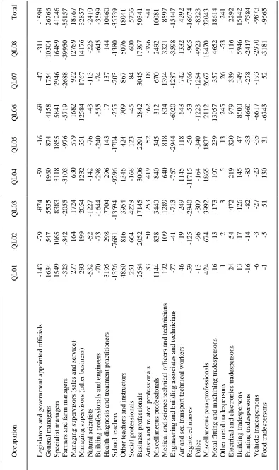
3.2 Employment by Qualification Field
Table 5 shows the changes in the distribution of employment between persons with various qualification fields for the three simulations. It is to be interpreted in the same way as Table 1 for qualification levels. It would be possible to identify the occupational contributions for each qualification field separately, just as they were for the qualification levels in Tables 3 and 4. However, as the nature of the analysis has already been amply illustrated, an exposition at the same level of detail will not be repeated. In any case, the preceding discussion of qualification levels can also be applied to an understanding of some of the important results for qualification fields.
Of the 47 qualification fields listed in Table 5, the difference between the level of employment in the forecast and historical simulations exceeds ten thousand persons in seven cases, namely:
• QF00 No post-school qualification (22987+12296=35283 persons),
• QF72 Building construction (+31575),
• QF64 Mechanical engineering (+27726),
Code Description Historical Forecast APEC Simulation Simulation Simulation
QF11 Management 9276 5637 -634
QF12 Management support services 1264 -3089 -1052
QF13 Sales and marketing 5135 5930 -387
QF14 Financial services 6481 13114 -1514
QF21 Medicine -1037 -8781 -237
QF22 Nursing 3469 -17681 -270
QF23 Health Science 5668 -789 -80
QF24 Dental science 5041 762 -85
QF25 Veterinary studies 525 -188 40
QF29 Other health 720 235 -59
QF31 School teacher training 6031 -18338 -1895
QF32 Post-school teacher training 286 -391 -101
QF39 Other teaching 930 -832 -97
QF41 Behavioural studies 13061 4518 -441
QF42 Welfare 15782 4824 -165
QF43 Librarianship -98 350 -86
QF44 Language and area studies 2871 532 -283
QF45 Religion and philosophy 2177 -1428 -64
QF46 Economics 2980 2617 -240
QF47 Law 6118 3633 -423
QF48 Visual and performing arts 4949 2462 -551
QF49 Other society and culture 4950 768 -249
QF51 Life science 4843 1638 -128
QF52 Physical science 5985 1688 -349
QF53 Mathematics and statistics 3017 1676 -189
QF54 Computer science 16339 11368 -551
QF59 Other natural science 1886 522 3
QF61 Surveying and cartography -1962 -1799 -92
QF62 Civil engineering -1515 -1203 -285
QF63 Electrical & electronic engineering -19339 274 -2254
QF64 Mechanical engineering -39877 -12151 -4224
QF65 Metallurgical & mining engineering 80 948 -172
QF66 Printing -4050 -3480 -272
QF67 Automotive engineering -11872 -5156 318
QF68 Textiles, clothing and footwear -2255 -923 -400
QF69 Other engineering -3176 1496 -775
QF71 Building design 240 218 -181
QF72 Building construction -20270 11305 -476
QF79 Other architecture and building -735 19 -3
QF81 Agriculture -5746 -4298 4392
QF82 Horticulture -213 278 331
QF89 Other Agriculture & related fields -149 -183 27
QF91 Hairdressing and beauty therapy 840 -7460 -759
QF92 Food and hospitality services 1374 -4956 -154
QF93 Transport -4433 -4190 21
QF99 Other miscellaneous -3290 -2480 -55
QF00 No post-school qualification -12296 22987 15097
• QF22 Nursing (-21150),
• QF63 Electrical and electronic engineering (+19613), and
• QF42 Welfare (-10958).
The unskilled category is, of course, common to both the qualification level and qualification field classifications, and the occupational breakdown presented in Section 3.1.3 remains relevant. Of the remaining six categories, three (QF72, QF64 and QF63) fare better in the forecast simulation because of their association with the construction sector, and three (QF31, QF22 and QF42) fare worse because of their association with the government-dominated industries
Education, Health and Welfare and community services. The factors
influencing employment opportunities in all these industries have been canvassed in Sections 3.1.1 and 3.1.2. Note that persons with qualifications in the field QF54 Computer science are heavily concentrated in the occupation
Computing professionals; hence the earlier explanation of the relatively poor
employment prospects in the forecast simulation for the occupation also pertains to the qualification field.
3.3 Employment by Age Group
Table 6. Employment Changes by Age Group, Persons
Age Group Historical Forecast APEC Simulation Simulation Simulation 15 to 19 -1130 2529 1533 20 to 24 1035 2209 645 25 to 34 2254 -344 -1040 35 to 44 5061 -2026 -1255 45 to 54 -2731 -1602 -146 55 to 64 -4645 -696 166
65+ 156 -70 97
Total 0 0 0
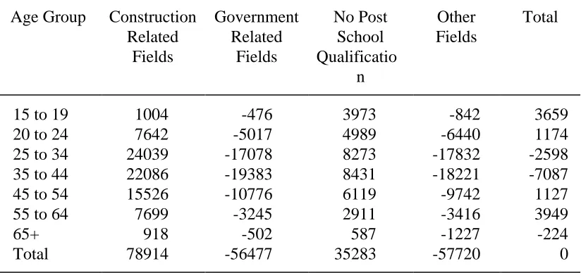
Table 7 shows the age by qualification matrix obtained by taking the difference between the corresponding matrices for the forecast and historical simulations. In this matrix the qualification fields of Table 5 have been aggregated into four groups: the Construction related fields (QF72, QF64, and QF63), the
Government related fields (QF22, QF31 and QF42), the No post-school qualifications field (QF00) and all other fields. For reasons already canvassed,
the employment opportunities for persons with construction-related qualifications or with no post-school qualifications are better in the forecast
Table 7. Employment Changes by Age Group and Qualification Field Forecast Simulation minus Historical Simulation, Persons
Age Group Construction Government No Post Other Total Related Related School Fields
Fields Fields Qualificatio n
simulation than in the historical simulation, while the opportunities of those with government-related qualifications are worse. For persons with other qualification fields taken as a group, the differential impact of the two simulations is quite similar to that for persons with government-related qualifications. Bearing in mind the decomposition in Table 7, the differences between the historical and forecast simulations in Table 6 can now be understood in terms of our preceding discussion.
3.4 APEC Simulation
The direct effect of the APEC trade liberalisation initiative is to change the prices (measured in domestic currency) that Australian economic agents receive for their exports and pay for their imports. On the export side, the removal of tariffs and non-tariff barriers on Australian processed food products, especially in Japan, is the most important development. For given prices paid by foreign consumers, the prices received by Australian producers increase. Hence the output of food products, and of the primary agricultural commodities which supply inputs to food processing industries, increase strongly. Against this, the removal of protection against foreign commodities in Australian markets causes the competitive position of some import-competing industries to deteriorate, with consequent reductions in output and employment. The industries most seriously affected are Textiles, clothing and footwear and
Passenger motor vehicles. It turns out that, on balance, the world prices of
Australia's exports increase relative to the world prices of its imports, i.e., Australia's terms of trade improve, providing a net stimulus to production and employment in Australia.
Two aspects of our employment results for the APEC simulation stand out. Firstly, although the period of adjustment is similar to that for the historical and forecast simulations, the size of the adjustment is generally much smaller. Hence, when considering the need for different types of training, the role of trade liberalisation may tend to be overemphasised if it is not carefully located within a more comprehensive analysis of the factors driving structural change. Secondly, in Australia's case at least, the role of the agricultural sector is crucial. From Table 5, only two of the 47 qualification fields benefit from significant employment redistributions, namely, QF81 Agriculture and QF00
No post-school qualification. Moreover, only two of the 52 ASCO minor
groups benefit from the redistribution across occupations14, namely, 14
Farmers and farm managers and 89 Miscellaneous labourers and related workers. An examination of the redistribution between the ASCO unit groups
shows that it is farm labourers that are responsible for the favourable outcome for the latter minor group. Because most farmers and farm labourers do not hold post-school qualifications, agriculture also lies behind the favourable outcome for unqualified workers in category QF00.
The increase in the employment share of agricultural workers is achieved mainly at the expense of workers in other export-oriented and import-competing industries. As those industries together employ a broad mix of occupations and qualifications, the reductions in employment induced by the trade liberalisation are also broadly distributed across occupations and qualifications. From Table 5, the qualification fields for which employment contracts the most are QF63 Electrical and electronic engineering and QF65
Mechanical engineering. Both are associated with import-competing
manufacturing industries via the occupations 41 Metal fitting and machining
tradespersons, 42 Other metal tradespersons and 43 Electrical and electronics tradespersons. Note that, notwithstanding the depressing effect of the currency
appreciation on the tourism industry, the qualification field QF93 Transport is one of the few to expand its employment share. This is because trade liberalisation leads to an increase in the share of international trade (both exports and imports) in GDP, and hence to an increase in the margins usage of transport services. The positive result for the field QF67 Automotive
engineering is associated with the repair, rather than the production, of motor
vehicles.
14 To conserve space, the redistribution of employment across occupations for the APEC simulation is
4. Concluding Remarks
The necessity for a nation's workforce to keep pace with the demands of a productive system faced with rapid technological and social change provides a compelling rationale for the notion of lifelong learning.15 In this paper, the notion has been imbued with a quantitative dimension by analysing the effects of such changes, as represented by changes in the distribution of employment across occupations, on the demand for labour with different qualification levels and fields. That is, computations have been conducted with a view to determining which qualifications might usefully be targeted by the providers of lifelong learning programs. Using the Australian economy as a case study, three different redistributions have been analysed, one concerned with historical changes, one with prospective future changes and one with changes induced by trade liberalisation. The analysis suggests three conclusions about the relationship between structural change and the provision of training services.
Firstly, the economic forces driving structural change are numerous and diverse, and their net effect on the demand for labour is not transparent. Hence generalisations and "stylised facts" are likely to be of only limited usefulness in determining training priorities. For example, according to the analysis, there is no secular tendency for structural change to favour the employment of persons with higher level qualifications, at least over the time periods and range of qualifications considered here. Similarly, structural change does not systematically favour the qualifications of the young over those of the old. For Australia, trade liberalisation shifts employment away from "professional, technical, administrative and managerial occupations" and into agriculture, the opposite of the effect thought likely to pertain by the OECD. This is not to say that the stylised facts are inoperative, but only that their effects are diluted and scrambled by the presence of other important influences such as the business cycle, government policy and international comparative advantage.
Before proceeding, it is appropriate to remind the reader that the present results are conditional on the assumptions incorporated in the analysis. In particular, the analysis abstracts from
15 Although compelling, the utilitarian motivation is not the only one to have been advanced in the
• changes over time in the distribution of qualifications within a particular occupation and
• changes over time in the distribution of skills within a particular qualification level.
These limitations are potentially important. For example, between 1989 and 1994 the number of students engaged in higher education in Australia increased by 32.7% whereas the number of persons in the labour force increased by only 7.6%. This suggests that the share of persons with higher level qualifications in an occupation has been tending to increase.16 While the analytical framework can accommodate less restrictive theoretical specifications readily enough, data availability has precluded their empirical implementation in the present study. For that reason, some of our results should be regarded as indicative rather than definitive.
In addition to being numerous and diverse, the forces driving structural change are also interconnected. The demand for labour of a particular qualification depends on employment in the occupations that use the qualification relatively intensively. Employment in a particular occupation depends on employment in the industries that use the occupation relatively intensively, and on changes in the distribution of employment across occupations within those industries. Employment in a particular industry depends on the output of the industry, on its rate of capital formation and on various kinds of technical change. The output of an industry depends, inter alia, on the state of the macroeconomy, on government policy, on the terms of trade and on social change such as population ageing. To determine the effect of structural change on the demand for a qualification, therefore, one must not only specify the nature and magnitude of the economic forces operating at each level of this hierarchy but also how a change at one level affects the outcome at other levels. This kind of determination lies outside the range of qualitative analysis. In other words, if the concept of lifelong learning is to contribute to the efficient (from the utilitarian point of view) allocation of resources for training, it must be married with formal modelling techniques.
Finally, the formal modelling techniques should ideally be forward looking.
16 To complicate the matter further, the rapid increase in the number of students in higher education
For training purposes, it is mandatory that the future demand for labour of different types be forecast in one way or another. It takes time to conduct a training course and the skills that result are generally expected to retain their social usefulness for an extended period after the completion of the course. Formal labour market forecasting is an uncertain activity, but the uncertainty is not diminished by a reliance on qualitative methods for extrapolating historical experience into the future.
References
Adams, P.D., P.B.Dixon, D.McDonald, G.A.Meagher and B.R.Parmenter (1994), "Forecasts for the Australian Economy Using the MONASH Model",
International Journal of Forecasting, 10, 557-571.
Adams, P.D., K.M.Huff, R.McDougall, K.R.Pearson and A.A.Powell (1996), "Medium- and Long-Run Consequences for Australia of an APEC Free-Trade Area: CGE Analyses Using the GTAP and MONASH Models", Centre of Policy Studies, Monash University, mimeo (forthcoming in Asia
Pacific Economic Review).
Access Economics (1996), Economics Monitor, Canberra.
Australian Bureau of Statistics (1987), The ASCO Dictionary, Australian Government Publishing Service, Canberra.
Australian Bureau of Agricultural and Resource Economics (1996), Economic
Outlook, Australian Government Publishing Service, Canberra.
Candy, P.C. and R.G.Crebert (1991), "Lifelong Learning: an Enduring Mandate for Higher Education", Higher Education Research and Development, 10 (1), 3-17.
Candy, P.C., R.G.Crebert and J.O'Leary (1994), Developing Lifelong Learners
through Undergraduate Education, National Board of Employment,
Education and Training, Commissioned Report No. 28, Canberra.
Dixon, P.B., and D.McDonald (1993), An Explanation of Structural Changes in
the Australian Economy: 1986-87 to 2002-03, Background Paper No. 29,
Economic Planning Advisory Council, Canberra.
Dixon, P.B., J.Mennon and M.T.Rimmer (1996), "A General Equilibrium Explanation of the Rapid Growth in Australia's Trade", paper presented to the Economic Society of Australia, 25th Annual Conference of Economists, Canberra.
Dixon, P.B. and M.T.Rimmer (1996), "MONASH Forecasts of Output and Employment for Australian Industries: 1994-95 to 2002-03", Australian Bulletin of Labour, 22(4), 237-264.
Hertel, T.W. (ed, 1997), Global Trade Analysis: Modeling and Applications, Cambridge University Press, New York.
Meagher, G.A. (1997), "The Medium Term Outlook for Labour Demand: An Economy-Wide Assessment", in Changing Labour Markets: Prospects for
Productivity Growth, Industry Commission, Melbourne.
Organisation for Economic Co-operation and Development (1996), Lifelong
Learning for All, OECD, Paris.