Development and testing of a variable valve timing system (VVT) for a twincam automotive engine

FTS THESIS

629.252 COS

30001007614367

Cosic, Ivan

Development and testing of a

variable valve timing system

A C K N O W L E D G E M E N T

I would like to gratefully thank m y supervisor, Kevin Hunt and m y co-supervisor

M a r k Armstrong for their valuable guidance, patience and advice. Without their

support this project would not have been possible.

I am grateful to Professor Geoffrey Lleonart for his patience and advice in the

correction of m y thesis.

I wish to thank the technical staff at the School of Built Environment, especially

Laurance Martin and Harry Friedrich for constructing the cylinder head test rig and

practical assistance.

I wish to thank Bruce Cameron from Holden Australia for his kind donation of a

Holden Vectra 2.0 litre twincam engine for the project.

I am thankful to MSC Software for their support and advice in ADAMS software.

Finally, I would like to thank my entire family for their support.

TABLE OF CONTENTS

ABSTRACT

1. INTRODUCTION

1.1 Background

1.3 Aim

2.1 Introduction

2.2 Phase Changing

1.2 Variable Valve Timing 3

4

1.4 Approach 4

2. L I T E R A T U R E R E V I E W 5

5

5

2.3 C a m Changing 1 0

2.4 Intake Valve Closing !5

2.5 Lost Motion Valves 18

2.6 Electrically Actuated Valves 19

2.7 Hydraulically Actuated Valves 20

2.8 Valves Actuated by T w o Cams in Parallel 21

2.9 Literature Review Summary 22

3. METHODS AND EQUIPMENT 23

3.1 Introduction 23

3.2 Engine Specification 23

3.6 Vectra Engine Cylinder Head Valve Profile

3.7 Hertzian Contact Theory 30

4. RESULTS AND DISCUSSION

33

33

39

47 4.1 Computer Simulation

4.2 DVC Components

4.2.1 Constraints

4.3 Dynamic Valve Control

4.4 Simulation Results

4.4.1 DVC Valve Profile 52

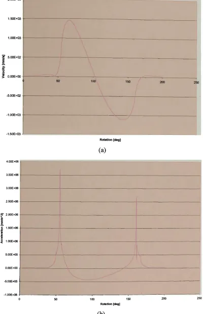
4.4.2 Valve Velocity and Acceleration Results 69

4.5 Force and Stress Analysis of Components 81

4.5.1 Forces Acting on DVC Components 82

4.5.2 Stress Analysis 93

4.5.3 Hertz Contact Pressure "

5. CONCLUSIONS AND RECOMMENDATIONS 100

5.1 Conclusions 10°

ABSTRACT

Variable valve timing ( W T ) is an innovative design that enhances automotive engine

performance and is important in addressing fuel consumption and emission output

concerns. The purpose of the research reported here w a s to examine the concept of a

W T system because it had the promise of application in the advancement of engine

technology.

In this study, a new WT system, termed the dynamic valve control (DVC) system

w a s developed. The D V C system w a s modeled using the computer simulation

software package A D A M S , which determined the forces acting on the principal

components at operational speeds, as well as the valve timing and lift profile of the

system. Stress analysis of the rocker arm w a s carried out using Cosmos/DesignStar

software. The valve timing and lift characteristics of the D V C system were compared

to an existing standard production engine.

The results of the study showed that the proposed DVC system can essentially realise

closure of its valves and achieve variable valve lift. In addition, the D V C system

valve timing and lift profile showed better characteristics w h e n compared with those

1. INTRODUCTION

1.1 Background

Resources of fossil fuels are finite and if they are to be used to provide energy for transport

they must be used efficiently. There are also strong pressures to m a k e automotive vehicles

less environmentally polluting and one of the most important factors in reducing global

warming is the increased use of vehicles with better fuel economy. T h e U.S Department of

Energy (1998) concluded that for every litre of fuel burnt in a vehicle, 9 kilograms of carbon

dioxide, a greenhouse gas pollutant, is transferred into the atmosphere. B y choosing a vehicle

with a fuel consumption of 50 kilometres rather than 4 0 kilometres per litre can prevent

approximately 10000 kilograms of carbon dioxide from being released over the lifetime of a

vehicle.

About 15% of the energy in the fuel is used to propel a vehicle, the rest of the energy is lost

to atmosphere. Automobiles need energy to accelerate, and to overcome air resistance and

the friction from tires, wheels and axles. Fuel provides the needed energy in the form of

chemicals that can be combusted to release heat. Engines transform heat released in

combustion into useful w o r k that ultimately turns the vehicle wheels, propelling it along the

road, see U.S Department of Energy (2001).

Over the last decade there has been a significant improvement in the fuel consumption of

vehicles and as a result they have b e c o m e less polluting. T h e most effective w a y to increase

horsepower and /or efficiency is to increase an engine's ability to process air. Since the

engine valves play a major role in controlling the flow of air/fuel mixture into and out of the

cylinders, it is important to study the role of engine valve systems in relation to improving

the efficiency of automotive engines.

Valves activate the airflow of an automotive engine. The timing of air-intake and exhaust is

controlled by the shape and phase angle of cams. T o optimise the air-flow, engines require

different valve timings at different speeds, and it has been found beneficial to open the inlet

intake and exhaust periods should be increased as the engine speed increases.

Overlap refers to the period when both the intake and exhaust valves are open at the

same time. W h e n the intake valve is opened before the exhaust valve closes, a scavenging

effect occurs, in which the rush of the exhaust out of the cylinder draws in a little m o r e of the

intake charge into the cylinder.

The valves of an engine do not open and close exactly when the piston reaches the top and

bottom of its cycle. T h e intake valve begins to open before the piston reaches top dead centre

( T D C ) , and closes after the piston reaches bottom dead centre ( B D C ) . The exhaust valve

begins to open as the piston reaches the bottom, and begins to close as the piston reaches the

top. A s the engine's speed increases, air in the manifold gains m o m e n t u m , and even w h e n

the piston reaches B D C , air continues to be drawn into the cylinder. Thus, to obtain as m u c h

air as possible in the cylinder without causing inefficiencies from inertial forces, it is

desirable to have the valve timing change with the engine speed.

Previously, manufacturers have used one or more camshafts to open and close an engine's

valves. T h e camshaft is turned by a timing chain connected to the crankshaft and as the

engine speed increases or decreases, the crankshaft and camshaft rotate to keep the valve

timing close to that needed for engine operation. Increased valve duration (the length of time

that the valves are held open) yields greater power at high speed but reduces torque at low

speed. While a greater valve lift (distance that the valves are opened, usually expressed in

millimetres) without increasing duration, yields m o r e power without m u c h change in the

nature of the power curve. Generally it is impractical to optimise the valve timing for both

high and low engine speed with a simple crankshaft-driven valve train. A s a result, engine

designers have to compromise timing in the specification of the camshaft. For example, an

ordinary sedan has its valve timing optimized for mid-range engine speed so that both low

speed driving ability and high-speed output do not significantly suffer. However, this

1.2 Variable Valve Timing

A s technology has advanced, so too has the development of engine design and nowadays it is

normal for modern vehicles to have multi-valve technology. Variable valve timing ( W T ) is

seen as the next step to enhance engine efficiency.

Variable valve timing was first introduced as an innovative design that increased engine

torque and output while addressing environmental issues, such as pollutants emitted from

automotive engines. T h e variable valve timing system uses an electronic system, k n o w n as

the engine control unit ( E C U ) to electronically control the operation of the engine valves.

The system is able to detect the engine speed and adjust the valve timing accordingly. A s a

consequence, m o r e oxygen can be supplied through the air intake valve as more fuel is

injected into the combustion chamber. Greater fuel and oxygen in the combustion chamber

leads to increased power and torque.

Most variable valve timing systems are combined with lift control, which varies the lift of the

intake and exhaust valves while the engine is operating at high speed. A s the intake and

exhaust valve lift increases, a larger volume of air/fuel mixture is introduced, along with

ejection of a greater volume of exhaust gas. This results in the engine producing higher

output power while operating at high speeds. T h e variable valve timing system allows the

valve timing of an automotive engine to be ideally fixed by increasing the valve lift w h e n the

engine speed is high, which results in improved fuel economy.

In principle, variable valve timing improves fuel efficiency and performance because it

adjusts the valve timing between high and low engine speeds for optimum performance, thus

efficiency throughout the entire speed range can be improved.

The variable valve timing system proposed in this study called the dynamic valve control

system ( D V C ) is a unique system based on the concept of varying the degree of valve lift, the

duration of valve opening and capable of virtual closure of the valves.

1.3 A i m

The aim of the research program reported here w a s to develop a computer based model of a

variable valve timing system, developed by m y co-supervisor M a r k Armstrong, called

dynamic valve control ( D V C ) for automotive engines.

1.4 Approach

The present study represents the initial stage of a research and development program

involving the design and construction on an experimental D V C system to be fitted to an

existing automotive engine.

To achieve this aim a computer simulation model showing the operation of the DVC system

was constructed using A D A M S software. This virtual model was used to establish a

geometry that improves engine performance. The forces acting on the rocker arm of the D V C

system were analysed, enabling the design of this component to be refined. In addition, the

valve timing and lift characteristics of a current production engine were compared to the

2. LITERATURE R E \ T E W

2.1 Introduction

Many mechanisms have been proposed to produce variable valve timing systems. Each

mechanism varies the valve timing either in duration, phase, or both. There are numerous

versions of W T mechanisms in production today, and these W T systems can be basically

classified into seven W T models, which are reviewed below.

2.2 Phase Changing

Cam phasing WT is the simplest, cheapest and most common mechanism used presently.

Basically, it varies the valve timing by shifting the phase angle of camshafts relative to the

crankshaft. Wilson et al. (1993), concluded that intake and exhaust camshafts can be

simultaneously varied with notable improvements in fuel economy and emission reduction,

this w a s also confirmed by Ashley (1995).

The phase angle can be shifted either by the use of a phasing actuator, whereby the change in

phase angle is produced by adjusting the hydraulic flows in and out of the actuator chambers

or with the camshaft drive being connected to the camshaft through a helical spline. The

latter mechanism w a s employed by M a e k a w a (1989). The phase angle between the

driveshaft and the camshaft w a s changed as the idler gear w a s moved axially along the

camshaft or vice-versa.

Wilson et al. concluded that high performance double overhead cam (DOHC) engines had a

long valve open duration, high valve lift and produced m a x i m u m power output. However,

the large valve overlap caused poor idle stability and also reduced engine torque at low

Moriya et al. (1996) developed the Intelligent Variable Valve Timing ( W T - I ) , as depicted in

Figure 2.1. The W T - I system varies the valve timing by shifting the phase angle of

camshafts and only responds w h e n the valves open and close in relation to engine speed. It

basically consists of three parts:

Crank Position Engine Oil P u m p Sensor

Figure 2.1 - W T - 1 system

(1) WT-I Pulley - Located at the front end of the intake camshaft, it produces a timing

difference between the intake camshaft and the crankshaft by a hydraulic actuator.

(2) Oil Control Valve (OCV) - Controls oil pressure to the WT-I pulley according to ECU

c o m m a n d and continually controlling oil feeding and draining between the W T - I Pulley

and O C V achieves continual phasing.

(3) Engine Control Unit (ECU) - Computes optimal valve timing based on the engine

operating condition and drives the O C V . The O C V control current is determined by

Titolo (1991) investigated the use of a Fiat W T system for use in a V 8 engine. T h e W T

device comprised :

(1) A multi-dimensional cam-follower assembly

(2) An actuator regulator assembly

The multi-dimensional cam follower varies the valve opening/closing, both in phase and in

lifting. T h e actuator regulator assembly changes the cam-follower position by means of an

axial displacement of the camshaft, which takes place continuously as a function of engine

speed.

When the engine is running, the rotation of the camshaft begins to open the intake or the

exhaust valve. At the beginning of valve opening, an oscillating plate is in a nearly

horizontal position. A s the valve lift increases, the plate changes its inclination until it

assumes the m a x i m u m inclination at m a x i m u m lift. During the valve-closing phase, the

m a x i m u m plate inclination returns to a horizontal position.

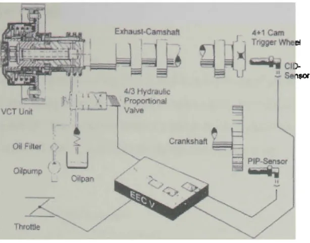
Steinberg et al. (1998) developed a fully continuous variable camshaft timing (VCT) system

which can be applied to both intake and exhaust camshafts. T h e V C T system is shown in

Figure 2.2.

Figure 2.2 - V C T system

Sensors and triggerwheels are used to measure the camshaft position relative to Top

D e a d Centre ( T D C ) . T h e engine management system processes these data to continuously

control the c a m position via an electric current to the solenoid.

A cylindrical component, which has helical gears on its exterior and interior surface, is fitted

between the camshaft pulley and the camshafts end. The gear on the exterior surface meshes

with a corresponding gear in the bore of the camshaft pulley, while the interior gear meshes

with a gear mounted on the end of the camshaft. Opposite the camshaft, a piston is m o v e d

axially by oil pressure depending on the camshaft position. T h e axial m o v e m e n t is

transformed into a rotation of the camshaft relative to the timing pulley. Leone et al. (1996)

concluded that there were three benefits to the V C T system. Firstly, N O x is reduced due to

the increased internal residual, secondly, unburned Hydrocarbons are reduced because they

were drawn back into the cylinder to be "reburnt" during the next combustion cycle, and

Mitchell mechanical variable valve timing system. T h e system exploits angular velocity to

change valve timing.

The system can be seen in Figure 2.3, and it is the eccentricity of the driveshaft axis to the

camshaft axis that generates a change in valve timing by imposing a variable angular velocity

on the camshaft. T h e variation creates a phase lag and phase lead of the camshaft in relation

to the drive shaft that is exploited to change the valve timing.

C o m m o n driveshaft

, I Hollow camshaft L|nk

Figure 2.3 - Mitchell W T system

The Mitchell system can be applied to single or multi-cylinder engines with single or twin

camshaft configurations.

Yagi (1992) et al. developed a variable valve actuation mechanism called the shuttle cam.

T h e system, s h o w n in Figure 2.4, uses a gear-train-driven valve system with a rocker arm

that activates the valve. T h e c a m gears rotate around the idler gear and the camshafts m o v e

along the rocker-arm surface that are concentric with the idler gear. This enables variation of

lift by the alternation of the rocker-arm lever ratio and the c a m phasing changes

Figure 2.4 - Shuttle cam

A variable valve timing system called the VAST, was developed by Hannibal et al. (1998),

the system enabled the variable control of the intake and exhaust valves. It was possible to

vary the valve opening, up to approximately 50° crankshaft angle, continuously for each

valve lift movement. A s a result, fuel consumption and emissions were reduced.

Cam phasing WT systems, are simple and compact mechanisms that have minimal wear

and energy loss. H o w e v e r to date, they cannot vary the duration of valve opening, thus

allowing only earlier or later valve opening.

they allow variability in the duration of valve opening as well as the lift of the valves. They

can also switch between completely different c a m profiles, unlike other systems which can

only basically vary the timing by advancing and retarding a standard set of cams.

In 1989, Hosaka et al. (1991) introduced the valve timing electronic control (VTEC)

engine system, which w a s able to maintain a high output throughout the entire engine speed

range. Thus enabling the high speed performance of a racing engine without sacrificing low

and m e d i u m speed performance.

Heywood (1988) stated that to develop a high performance engine it is necessary to increase

the volumetric efficiency and reduce friction. A racing engine requires wider valve overlap

and increased valve lift to obtain optimum performance at high engine speed. H o w e v e r in a

conventional engine, the valve timing and degree of valve lift is set for optimum

performance at low and m e d i u m engine speeds.

Hosaka et al. (1991) identified that by designing for higher valve lift, wider valve timing and

larger valve diameter, it w a s possible to obtain a higher volumetric efficiency to cope with

high output engine speeds. With V T E C , the valve timing and lift can be adjusted at low

engine rotation to increase torque and prevent air from being forced back through the intake.

A diagrammatic view of the VTEC system is shown in Figure 2.5. The cam has three

separate profiles located at the intake and exhaust of each cylinder. T h e centre profile is used

exclusively for high speed and the t w o identical outside profiles for low speed.

® Camshaft ,=.,,. .. „

(Z} _{Hydraulic Piston A}

® C a m Lobe for Low Speed Range ® Hydraulic Piston B

® C a m Lobe for High Speed Rane e <g, S t o p p e r p j n

9> Primary Rocker Arm @ Lost-motion Spring

® Mid Rocker Arm & E x„a u s, V a | y e

© Secondary Rocker Arm @ ln,ake V a | v e

Figure 2.5 - V T E C system

The rocker arm assembly comprises a mid rocker arm with primary and secondary rocker

arms on each side. The changeover mechanism is composed of two hydraulic pistons that are

located within the rocker arm, a stopper pin and a return spring. A lost motion spring is

located within the mid-rocker arm, so that the valve can open and close at high speeds. The

whole system is operated by a hydraulic actuator, which is controlled by the engine control

the low-speed c a m and follows the high speed cam. This effectively allows the high-speed

c a m to control the t w o valve timings. Hosaka et al. concluded that since the high-speed cam

was able to control the t w o valve settings, the engine w a s able to get sufficient air at both

low and high speeds. A s a result, the engine w a s able to perform better with an even torque

band, and more than adequate power at the high end.

Matsuki et al. (1996) conducted further research of the VTEC system by developing a three

stage V T E C lean burn engine. The mechanism developed w a s based on the previous V T E C

system but included modifications to the valve train, intake port and combustion chamber

configurations. The three-stage V T E C system had the same the valve timing and lift

switching mechanism as its predecessor, the V T E C .

As illustrated in Figure 2.6, it can be seen that the three stage VTEC system's camshaft has

three c a m lobes per valve pair and rocker arms for primary, secondary and middle cam

profiles. The three profiles are for valve inactivity, low and medium engine speeds and high

engine speed. The rocker arm integrates two hydraulic passages, which can be switched to

and from each other by a spool valve setting.

Medium-speed switching piston

High speed switching piston

Y Medium-speedcam \ High-speed c a m Inactive c a m

At medium-speed range, the hydraulic passage opens as a result of the electronic control unit

( E C U ) signal, providing hydraulic pressure to the switching piston. The primary and

secondary rocker arms are connected to each other and lift the valve using the medium-speed

cam profile. The valve timing and lift at this stage are set so that they ensure an appropriate

charging efficiency and less valve drive friction.

While in the high-speed range, the ECU allows the other hydraulic passage to open,

providing hydraulic pressure to the high-speed switching piston. A s a result, both the primary

and secondary rocker arms are connected to the middle rocker arm. Consequently accessing

the high-speed c a m profile, the valve timing and lift are optimized to generate a high power

output.

They concluded that the three-stage VTEC system can generate approximately 40% more

engine power than the original V T E C engine that Hosaka et al. (1991) developed, while

maintaining the same fuel consumption. N a k a y a m e et al. (1994) concluded that because the

V T E C systems alter the valve timing and lift according to various driving conditions, it w a s

able to use a leaner mixture than existing engines. A s a result, the V T E C systems reduce

Hydrocarbon emissions considerably due to the improvement in engine combustion.

Hatano et al. (1993), developed a WT system featuring a multi-mode valve system, it was

called Mitsubishi Innovative Valve Timing and Lift Electronic Control ( M T V E C ) . The

system enables deactivation of unnecessary cylinders during low speed cruise and improved

the engine output performance under all engine speed ranges by selecting optimum cam

0 ACTIVATED • DEACTIVATED

MODE

I

I

I

CYLINDER

NO. 1,4

C Y U N D E R S H

NO. 1,3

CYUNDEfli.

ALL CYLINDERS

ALL CYLINDERS

CAM FOLLOWER

LOW. SPEED CAM HIGH • SPEED CAW

•

0

0

t

0

Table 2.1 - M I V E C valve operation

Hara and Kumaga (1989) developed a WT lift and timing control system (VLTC), which

varied the lift timing by changing the fulcrum of the rocker arm. The fulcrum w a s varied

according to the inclination of a lever that engages with a control cam. The control cam was

driven by an actuator mechanism to provide control over valve lift and timing. They

concluded that their system reduced valve train noise and delivered stable valve operation

throughout the high-speed range.

Although cam changing WT systems can vary the lift of the valves, they cannot fully close

the valves to zero lift, as well, additional cams are required to vary the lift from low-speed to

high-speed.

2.4 Intake Valve Closing

Intake valve closing is a practical concept applicable to engines in which the intake valves

can be phased relative to each other to extend the total intake opening period. Bassett et al.

eliminate most of the pumping losses (pumping loss represents the power required to p u m p

charge into and out of the cylinders) and conserve fuel. They identified that the problem of

pumping losses must be addressed, because as the engine w a s throttled, pumping losses

progressively increased until no useful output w a s generated at idle speed.

Their proposed system consists of an intake camshaft, which causes late closing of the intake

valve at all times. At high loads a reed valve situated in the intake manifold prevented the

charge from being rejected from the cylinder. At low loads, the reed valve w a s deactivated to

allow the charge to return to the inlet manifold. They asserted that the L r V C system allowed

the engine to operate with wider than normal throttle settings at low speed, thus enabling the

reduction of pumping losses.

Ma (1988) and Saunders et al. (1989) agreed with Bassett's research by also concluding that

there w a s better fuel consumption with the L I V C . Lenz and Wichart (1989) stated that with a

late intake valve closing mechanism, a torque increase of 8 % can be achieved, fuel

consumption can be improved by 4 % , along with and a 2 0 % - 5 0 % reduction in pumping

losses.

Payri et al. (1984) compared pumping losses between a standard engine and an engine fitted

with a W T system. Their conclusion w a s that pumping losses would be significantly

reduced with a W T system and the efficiency of an engine would improve. They found that

there w a s a strong pressure drop in the throttle valve of the carburetor w h e n the engine runs

at a partial load rate, this decreased the m e a n pressure along the intake and as a result,

pumping losses were increased. With a W T system, the throttle valve w a s eliminated and

load regulation w a s achieved by means of the total opening time of the intake valve. The

pressure drop during the intake process w a s minimal and the fluid inside the cylinder

expands from the m o m e n t that the intake valve w a s closed until the piston reached bottom

dead centre ( B D C ) and afterwards w a s compressed during the compression stroke.

of the engine after the required amount of charge has been induced into the cylinder. H e

found that compared to a conventional throttled engine operating at part load, the E I V C

had lower pumping loss, fuel consumption and N O x emissions. O n the other hand, Hara et al.

(1989) found that even though pumping losses were reduced with intake valve closing

mechanisms, improvement in fuel economy equivalent to the reduction in pumping losses

were not obtained. They concluded that the major contributing factor to this phenomenon

w a s the deterioration of the combustion. T h e cause of combustion deterioration w a s the drop

in cylinder gas temperature and pressure due to a decrease in the compression ratio.

Urata et al. (1993) found a solution to the combustion deterioration problem by developing a

hydraulic variable valve train ( H V T ) , which could vary the intake valve closing timing

freely. D u e to the fact that conventional engine management systems are not applicable for

non-throttling operation, they designed the H V T system, which could minimise pumping

losses and reduce fuel consumption.

A solenoid valve, was connected to the oil path, which linked the intake valve and cam to

block and release oil pressure. T h e valve lifted along its c a m profile once the soleniod valve

w a s activated. W h e n the solenoid-valve w a s activated to close during c a m lift, the valve was

lifted along the c a m profile as in conventional engines. W h e n the solenoid-valve w a s

deactivated to open at a specific time during c a m lift, oil pressure w a s released to let the

valve spring close the intake-valve, regardless of the c a m lift. Adjusting the time at which the

solenoid-valve opens, controlled the intake-valve closing timing.

Vogel et al. (1996) investigated implementing variable valve timing systems using a

secondary valve in the intake tract, which would act in accordance with the conventional

poppet valve of the engine. They found that there were t w o beneficial uses of the secondary

valve. Firstly, it enabled the control of valve overlap, thus improving low speed and low end

performance. Secondly, to use it as a load control mechanism, i.e., it would replace the

conventional throttle and reduce pumping losses that were associated with conventional

throttling. O h y a m a and Fujieda (1995) stated that by substituting the throttle with direct fuel

injection, increases the air/fuel ratio limit, thus reducing nitrogen oxide emissions.

2.5 Lost Motion Valves

Lost motion valves are operated directly by conventional cams and the timing variation is

produced by varying the length of the pushrod to produce an adjustable lash in the valve

mechanism. The rocker fulcrum or the camshaft is m o v e d to vary the valve lash. Since these

mechanisms convey output motion during only part of the c a m lift, they are called

"lost-motion" mechanisms. Lost motion mechanisms are very simple to implement and can be

used to attain very ranges of valve opening. Systems can be designed that automatically vary

duration with engine speed to provide near-optimum full throttle fuel efficiency and torque.

Herrin and Pozniak (1984) found that their lost motion mechanism, termed a variable timing

lifter ( V T L ) , can vary the timing of engine valve opening and closing, w a s durable and

precise in its control. W h e n applied to a high specific output engine, the mechanism allowed

m u c h lower idle speeds and reduced idle fuel consumption without compromising

high-speed power. The V T L can minimise the effects of fixed valve timing compromise by

providing a reduction in valve open duration and valve overlap at low engine speeds to allow

a slow and stable idle, which reduced idle fuel consumption. The device however, responds

only to engine speed and cannot optimize valve timing for changes in load.

Lee et al. (1995) developed the electronic valve timing (EVT) system that operated with a

lost motion hydraulic actuator linked to a high flow electromagnetic solenoid valve. Valve

control w a s provided by an electronic control unit, which acted upon the solenoid.

W h e n the solenoid w a s closed, a hydraulic lock w a s created and the valve motion w a s forced

to follow the c a m profile. If the solenoid w a s opened during the valve event, the valve lift

and duration were modified depending on w h e n the solenoid w a s opened. They also obtained

similar results to Herrin and Pozniak. They concluded that by advancing the intake valve

closing timing, torque can be improved at low speed condition by about 1 0 % , fuel

by electronic triggering of the solenoid valves) from the linkages to effect lost motion

between the c a m s and the engine valves. This allowed optimization of valve timing, lift and

duration for retarding and for positive power.

Lost motion systems are one of the simplest mechanisms for obtaining a large range of valve

durations, however, the valve lift off and seating impacts of valves can cause high valve

stresses and engine speeds are limited by the seating impacts.

2.6 Electrically Actuated Valves

Electrically actuated valves are operated directly by electric actuators, usually solenoids.

Varying the time of energizing and de-energizing the solenoids produces variation in the

timing.

Schechter and Llevin (1996) introduced a camless engine with independent and continuously

variable control of valve timing, lift and duration. T h e engine valve opening and closing w a s

controlled by t w o solenoid valves that were connected to high and low pressure plenums.

Valve opening w a s controlled by the solenoid valve connected to the high pressure plenum,

while valve closing w a s controlled by the solenoid valve connected to the low pressure

plenum.

Douglas (1997) developed an electromagnetic valve actuator (EVA) system that controls

valves electronically, without the need for a camshaft, rocker assembly, pulley or timing belt.

The E V A system had one actuator at each valve chamber with t w o opposing spring coils

fitted at each valve chamber providing the necessary force to open and close the valves. The

spring forces were supplemented by electromagnetic force from the E V A coils. T h e intake

and exhaust valves were independently computer controlled and timed, making it possible to

fine tune air/fiiel and exhaust flows to engine needs.

Electrically actuated systems have a high energy consumption with restricted valve duration

2.7 Hydraulically Actuated Valves

Hydraulically actuated valves are operated directly by hydraulic actuators, usually hydraulic

cylinders and the fluid is metered through either mechanical or solenoid valves.

Desantes et al. (1988) investigated the use of a hydraulically controlled variable valve timing

system, which utilised a hydraulic mechanism to open and close the valves. The system w a s

based on an axial lifting of the intake valve by a hydraulic plunger. The degree of early

intake valve closing depended on the engine running conditions, which were controlled by a

microprocessor. T h e microprocessor controlled an electrovalve, which discharged the oil

stocked under the plunger through the driven valve. The plunger w a s located at one end of

the rocker arm, which pivoted around the c a m contact point as fixed centre. The variable

closing of the intake valve depended on the m o m e n t at which the microprocessor ordered the

electrovalve opening and closure. The system is illustrated in Figure 2.7.

C a m Rocker arm

Pump —I Plunger

Crohn et al. (1990) were able to adjust the intake valve timing by the use of a hydraulic

-mechanical acting camshaft adjuster. T h e timing w a s adjusted, dependent on the load and

engine speed, by turning the intake camshaft using a hydraulic adjuster. The camshaft

adjuster w a s controlled in line with the engine speed and load by the fuel injection control

unit.

Hydraulically actuated systems are simple in their operation and have fewer mechanical

elements than most standard valve trains, however, they are prone to high fuel consumption

and limited m a x i m u m engine speed.

2.8 Valves Actuated by Two Cams in Parallel

In these systems, the valves are operated by two cams in parallel in such a way that the valve

displacement equals the larger effective displacement of either cam. Timing is varied by

changing the phase angle between each c a m and the crankshaft. The most c o m m o n

implementation of this concept employs a single c a m profile, which is actually m a d e up of

two separate cams that can be rotationally shifted relative to each other. T w o concentric

shafts usually drive the t w o cams. T h e outer camshaft drives one set of cams while slots in it

allow the second set of cams to project through from the inner shaft.

Kreuter (1998) developed a similar system called the Meta WH. It had two camshaft*,

which operate as opening and closing camshafts that rotated at the same speed and acted on

the intake valves via a follower and a transmission element. The opening camshaft w a s

driven directly by the crankshaft while the opening c a m drove the closing camshaft via a

gear drive. T h e gear drive allows a phasing between both camshafts in a range necessary to

vary lift and duration of the valves from zero to m a x i m u m . The valve lift function

corresponded to the s u m of the displacements of the t w o cams. These systems have large

valve duration ranges but are mechanically rather complex.

2.9 Literature Review S u m m a r y

The literature review indicates that variable valve timing systems presently available have

shortcomings. Principally, c a m phasing mechanisms cannot vary the duration of valve

opening and cam changing systems cannot achieve zero lift. Other mechanisms suffer from

3. M E T H O D S A N D E Q U I P M E N T

3.1 Introduction

This chapter describes the experimental procedure involved in obtaining the valve lift

profile of a cylinder head and the actual valve lift results. T h e measurement of the

standard Vectra valve lift provided a profile from which m a x i m u m valve velocity and

acceleration could be estimated. These estimations provided input for setting upper

limits for the D V C system. T h e standard production engine selected w a s a Holden

Vectra 2.0 litre twincam engine. T o obtain the valve lift profile of the Vectra engine,

the Vectra cylinder head w a s removed from the engine and fitted to a specially

designed cylinder head test rig. T h e cylinder head test rig, w a s built in the School of

Built Environment at Victoria University of Technology. A future D V C prototype

will be trialed o n the Vectra cylinder head test rig.

To obtain the Vectra's valve lift profile, data acquisition software, DTVEE and a

LB-12/72 laser displacement sensor were used to evaluate the valve lift characteristics of

the standard Vectra cylinder head. T h e engine specifications, the details of the

construction of the test rig, the description of the data acquisition and the laser

displacement sensor and valve lift results of the Vectra cylinder head are presented.

3.2 Engine Specification

Model

Displacement

Stroke

Intake Valve Diameter

Exhaust Valve Diameter

Output

Torque

Firing Order

Compression Ratio

Engine Management

Fuel

Holden Vectra

1998 cm

86 m m

32 m m

29 m m

100 k W

185 N m

1,3,4,2

9.6:1

Simtec 5.5

Premium Unleaded Fuel

Table 3.1 - Holden Vectra engine specifications.

3.3 Cylinder Head Test Rig

The test rig is shown in Figure 3.1. The cylinder head was removed from the Holden

Vectra engine and bolted to the test rig's railings. A variable speed motor, located at

the bottom of the test rig drives the valve gear of the cylinder head. The variable

Figure 3.1 - Cylinder head test rig.

Type

Model

Input

Output

M a x i m u m Amperes

Vari Speed Motor Control

WW2SS

230 V

0.7 kW

5.5

Table 3.2 - Specifications for the variable speed motor.

3.4 Laser Displacement Sensor

Once the Vectra cylinder head was fitted to the test rig, to attain the valve lift profile

analog signals as the valves opened and closed. T h e laser displacement sensor is

illustrated in Figure 3.2. T o accurately sample signals, the reference point of the

sensor needs to be positioned within 30 to 50 m m of the intended target. If the sensor

is positioned within the acceptable measuring range, the L E D indicator will indicate

an orange colour. If the sensor is not positioned within range, the L E D indicator will

show a red colour. T h e sensor specifications can be seen in Table 3.3.

The reference position of the sensor was positioned approximately 40 mm from the

valve seat. Once the reference position w a s positioned within the acceptable range of

the valve seat, the sensor w a s switched on and as the valve opened and closed the

sensor sampled the analog signals.

L A S E R O N

3wrrtv*STAB*.fTY l - D >ncbcasc*

i ;

-too l*0>

,2x o d S

mounting bow

1f-|23;)

43

xx+n Reterence posflion

~»»10,5*»-

Type

Model

Reference Distance

Measuring Range

Light Source

Wavelength

Spot Diameter

Linearity

Resolution

Analog Voltage

Analog Impedance

Zero - Point Adjustment Range

Response Frequency

Power Supply

Current Consumption

High - Resolution

L B - 12/72

40 m m

± 10mm

Infrared Semi-Conductor Laser

780 n m

1.0 m m

l%ofF.S

2 |im (at 60 ms) /15 \xm (at 2 ms)/

50 jam (at 0.15 ms)

± 4 V (0.4 V / m m )

100 Q

30 to 50 m m

D C to 3 k H z (at 0.15 ms) (-3 dB)/ D C to 200 Hz (at 2 ms) (-3 dB)/ D C to 6Hz (at 60 m s )

12to24VDC± 10%

120 m A maximum

3.5 D T V E E Software

After the laser displacement sensor sampled the analog signals as the Vectra valves

opened and closed, the data acquisition software, D T V E E w a s used to show the

digital readout from the analog signal of the laser. A computer program w a s written to

acquire, process and save the data gathered from the laser measurements of the valve

lift of the cylinder head.

Prior to the cylinder head test, the user has to enter to the program:

(1) The analogue to digital configuration information,

(2) Data panel information

The DTVEE program basically consists of three parts, analogue to digital conversion,

data panel box and the analogue to digital sample results, which is the c a m

displacement box as seen in Figure 3.3. In the analogue to digital conversion box, one

specifies the channel to be read, the gain and the rate of data acquisition. The

information from the analogue to digital configuration box and the data panel box is

then processed and the digital readout of the measurement of the valve lift is

File E * View Defeug Ftow Bevice jrt) Data DT DataAcs Dia*av Wiidwt Jjet>

"^l^lglal »l 1 tel?|g| alfclftlftl 1 Ml I tfk.l xlfrl I •>!•»!,

HEIE3

Formula

A/D Coring A j2.014*a Result *— •H Get Data Panel

File N a m e I —J

To File

f

-' C A M D I S P L A C E M E N T

L__J

d

Figure 3.3 - D T V E E Data Acquisition Program

3.6 Vectra Engine Cylinder H e a d Valve Profile

The valve lift data was saved as an ASCII file in DTVEE, and then processed in

Microsoft Excel.

A s illustrated in Figure 3.4, the m a x i m u m valve lift of the standard Vectra engine was

10 9 8 7 6 5 4 3 2 1 0

0 90 180 270 360 450 540 camshaft rotation [deg]

Figure 3.4 - Vectra cylinder head valve lift and valve duration of two successive

lifts.

The result shows that the Vectra engine has no variable lift capability by which the

valve can be operated to suit engine speed. Its speed range is a compromise between

high and low rpm. This due to the fact that the Vectra engine uses two camshafts,

which are turned by a timing chain connected to the crankshaft, to open and close it's

valves. Therefore, as the speed of the engine increases and decreases, the crankshaft

to camshaft synchronisation is maintained to keep valve timing relatively close to

what is needed for engine operation. As can be seen from the figure the maximum

valve lift of the Vectra engine is 9 mm.

For Hertzian contact stress theory, the following assumptions can be made, see D e e

(1992):

(1) at the point of contact the shape of each of the contacting surfaces can be

described by a h o m o g e n o u s quadratic polynomial in t w o variables,

(2) both surfaces are ideally smooth,

(3) contact stresses and deformation satisfy the differential equations for stress and

strain of homogenous, isotropic and elastic bodies in equilibrium,

(4) the stress disappears at great distance from the contact zone,

(5) tangential stress components are zero at both surfaces within and outside the

contact zone,

(6) normal stress components are zero at both surfaces outside the contact zone,

(7) the stress integrated over the contact zone equals the force pushing the t w o bodies

together,

(8) the distance between the t w o bodies is zero within but finite outside the contact

(9) in the absence of an external force, the contact zone degenerates to a point.

The two cylindrical bodies in the DVC system that come into contact, which are of

significant importance, are the guideshaft and gudgeon pin. The contacting surfaces

have the only line contact that does not have an obvious arrangement in existing

engines.

The m a x i m u m Hertzian contact pressure for two cylinders pressed together by a force

is given by the equation, see Shigley (1989)

IF

* = - (3.1)

Fmax

nbl

Where

pmax = M a x i m u m contact pressure,

F = Contact force,

b = Contact half width,

3. RESULTS A N D DISCUSSION

3.1 Computer Simulation

From Chapter 3, it was seen that the measured maximum valve lift of the Vectra

engine w a s 9 m m and the valve duration w a s 130 degrees. T o obtain a comparison

between the valve lift profiles of the Vectra engine and the proposed D V C system, the

D V C prototype w a s modeled using A D A M S , a virtual prototyping software, to attain

valve lift characteristics.

Virtual prototyping technology has made significant advances in recent years and

many companies are utilising the technology in the design of products such as

automobiles, aircraft, railway, defense and industrial machinery. Virtual prototyping

enables one to realistically simulate the full motion behavior of a mechanical system,

to detect component interference, evaluate levels of vibration in the system, predict

deflection of parts and determine loads and forces on components.

ADAMS is a widely used virtual prototyping software, and the DVC system was

modeled using A D A M S . A D A M S provides the user with the tools to build a virtual

prototype, to the test the virtual prototype and to validate the performance of the

virtual prototype against k n o w n measurements.

3.2 DVC Components

The design of the DVC components, the rocker arm and guideshaft are critical to the

performance of the system and the design rationale of these components were as

follows:

(1) provide an actuating lever to interact with the top of the original valve bucket with

minimal deviation of contact from the valve axis,

(3) provide a concave, circular arc surface concentric with the axis of the guideshaft

for contact with the pin,

(4) ensure the line contact pressure on the rocker arm does not exceed what is

considered acceptable for conventional valve train components,

(5) ensure internal stresses of the rocker arm do not exceed the fatigue limit of its

material,

(6) provide a base circle surface that results in close to zero valve lift as possible

during interaction with the gudgeon pin,

(7) provide a concave arc that results in valve acceleration no greater than the

standard Holden Vectra valve train,

(8) ensure the line contact pressure of the interacting gudgeon pin does not exceed

that of conventional valve train components.

The DVC components were designed to allow rninimum modification to the standard

Vectra cylinder head.

The proposed components were constructed using SolidWorks, which is a 3D CAD

modeling software and their shells were then imported into A D A M S . T h e components

that m a k e up the D V C system can be seen from Figures 4.1, 4.2, 4.3, 4.4, 4.5, 4.6 and

4.7. The components used are the same for the inlet and exhaust valves. T h e materials

chosen were similar to conventional valve train materials and Table 4.1 details the

Component

Bucket

Valve

Rocker A r m

Valve Crank

Rockershaft

Guideshaft

Conrods

Gudgeon Pin

Material

Steel

Steel

Steel

Steel

Steel

Steel

Aluminium

Alurninium

M a s s (kg)

0.049

0.042

0.0267

0.15013

0.05661

0.03269

0.00714

0.00968

Table 4.1-Component mass property and material

Figure 4.2 - Gudgeon pin (pink component) and rockerarm as modeled using

-3 *1\

Figure 4.4 - Guideshaft as modeled using A D A M S

EJ < a BJd S«i»U. B""- S.WW look B *

All the D V C components are rigid 3 D bodies, and the extrusion tool w a s used to

create the components. SolidWorks models begin with a 2 D outline, which is then

extruded in the third dimension to form a 3 D model. The type of extrusion used

determines the shape of the desired component.

The valve and the bucket were created by sketching a half cross section with one edge

of the sketch formed by the central axis of symmetry. The torus extrusion w a s then

selected and the cross section w a s extruded through 360 degrees around the central

axis. The crankshaft, rocker and conrods required the linear extrusion tool and

the edges of the geometry were chamfered, filleted, holes and bosses were added and

the solids were hollowed. For the guideshaft, three rigid bodies were joined to create

that component. First of all the shape of the guideshaft profile w a s created and the

rockershaft w a s attached to the profile. The guideshaft can be seen in Figure 4.4.

Once the parts were created, they were imported into ADAMS. The material and mass

properties of the components were defined and the components were then arranged in

their correct co-ordinate positions.

4.2.1 Constraints

In order to correctly simulate the model, once the parts were created and positioned

correctly, they had to be constrained, that is, constraints are used to specify part

attachments and movement. H o w the parts will be attached to one another and h o w

they m o v e relative to each other has to be defined. A description of all the constraints

used can be seen in Appendix B. Figure 4.8 shows the bucket and valve, the bucket

pushes the valve open, once the rocker arm pushes o n the bucket. The same figure

also shows the constraints between the bucket and the valve. A translational joint w a s

used between the bucket and ground, so that once the rocker arm pushes o n the

bucket, it will translate along a vector aligned with respect to the valve. However,

during a simulation run the bucket separated from the valve and the valve did not

Therefore a fixed joint w a s introduced to prevent the bucket and the valve from

separating from one another during simulation. Also a coil spring is used so that the

valve will be able to close, once it opens.

Figure 4.8 - Bucket and valve as constrained using A D A M S .

The rocker arm pushes the bucket, which in turn opens the valve, however, the rocker

arm can only push the bucket due to the gudgeon pin moving backwards and forwards

between the rocker arm and guideshaft profile. The gudgeon pin moves towards the

end of the rocker arm, which is towards the rocker shaft, this in turn allows the bucket

to be pushed by the rocker arm. Figures 4.9, 4.10, 4.11, 4.12, 4.13, 4.14, 4.15,4.16,

4.17 and 4.18 illustrate h o w the rocker arm, gudgeon pin, guideshaft, rockershaft and

Figure 4.9 - 3 D illustration of rockershaft and rocker arm

E h E * tfe" t"U JmiiaH fl»v«v» SaWngi Tooli tjsHp

J

Figure 4.13 - 3 D illustration of rockershaft, rocker arm, gudgeon pin and conrods

ft» E<a Jfrw Biid Simulate H'**" Sural look 1 M >

Figure 4.17 - 3 D illustration of rockershaft, rocker arm, gudgeon pin, conrods, valve crank and guideshaft

In order for the rocker arm to c o m e into contact with the bucket, so that the bucket

can push open the valve, a contact force needs to be applied between the rocker arm

and bucket. Before a contact force can be applied, the surfaces of the rocker arm and

bucket where the contact will occur must be specified. Originally the whole of the

rocker arm and the bucket w a s specified, however this proved to be a problem as the

rocker arm w a s constrained from pushing onto the valve. T h e problem w a s solved by

specifying only the point of contact rather than the whole component. Therefore the

tip of the rocker arm and top of the bucket were specified as the contact surfaces, and

a simulated contact force w a s applied. Also, a revolute joint w a s specified between

the rocker shaft and ground, so that the rocker arm w a s able to pivot d o w n onto the

bucket.

A problem arose when the contact surfaces of the gudgeon pin and the guideshaft

were specified, in that the gudgeon pin could not m o v e along the guideshaft profile,

namely along the activating curve of the guideshaft. This w a s due to the fact that

w h e n a contact surface is chosen, the number of points along the contact surface for

the contact force to function properly must be introduced. In this instance, too m a n y

points were allocated along the activating curve of the guideshaft profile and this

restricted the gudgeon pin's movement. A smaller number of points were designated

along the curve and the gudgeon pin w a s then able to m o v e between the guideshaft

profile and the rocker arm. Contact forces were then applied between the gudgeon pin

and rocker arm and between gudgeon pin and guideshaft.

The gudgeon pin is moved along the rocker arm and guideshaft profile by the valve

crank, which is connected to the gudgeon pin by the conrods. A s the valve crank

rotates, the pin is pushed backwards and forwards, with the amount of the valve lift

determined by the guideshaft position. B y changing the degree of rotation of the

guideshaft, the valve lift opening can be m a d e either larger or smaller. In order for the

Previously a fixed joint w a s introduced between the conrods big ends and the valve

crank. It w a s found that this prevented the conrods from rotating about the valve

crank, so instead of applying a fixed joint, a revolute joint w a s used so that the

conrods could rotate about the valve crank. T h e gudgeon pin w a s fixed to the conrods

little ends, and as the valve crank rotated, the gudgeon pin w a s able to m o v e

backwards and forwards, with the sandwiching contact forces preventing the gudgeon

pin from leaving the rocker arm or guideshaft.

3.3 Dynamic Valve Control

The system is operated by the rotation of the valve crank. A s the valve crank rotates,

the gudgeon pin, which is connected to the valve crank by the conrod's, moves

forwards and backwards along the guideshaft profile. Figure 4.19 illustrates the

gudgeon pin as it m o v e s forwards along the guideshaft and rocker arm.

It should be noted that in Figures 4.19 to 4.21, one of the conrods w a s m a d e invisible,

so that the m o v e m e n t of the gudgeon pin along the rocker arm and guideshaft could

be seen clearly. O n c e the pin reaches the activating curve of the guideshaft, it pushes

the rocker arm d o w n against the bucket, which in turn opens the valve, as illustrated

in Figure 4.20.

Figure 4.20 - G u d g e o n pin at the activating curve of the guideshaft

When the pin moves backwards along the guideshaft and rocker arm, the valve begins

Figure 4.21 - Valve closing as gudgeon pin m o v e s backwards along the guideshaft

Variable lift is achieved by the guideshaft, which is controlled by a hydraulic

mechanism, connected to the engine management system. The guideshaft profile

moves backwards and forwards according to engine speed and load, varying the

interaction of the gudgeon pin as it m o v e s backwards and forwards along the rocker

arm. The degree of valve lift is dependent o n the amount the guideshaft is rotated. At

idle, the pin only touches the initial portion of the actuation curve of the guideshaft,

this effectively opens the valve by a small amount. This small opening of the valve

substitutes for the throttle, a device in the engine that regulates the flow of air into the

cylinders.

The DVC system will have a continuously variable lift, this means that the valves will

be able to open to lifts of say, 5 m m , 6 m m or 7 m m , with stepless variation and does

not just open fully to its m a x i m u m lift.

guideshaft is positioned at seven degrees or at start location, while Figure 4.23

illustrates the D V C system w h e n the valve is fully opened, w h e n the guideshaft is at

357 degrees (three degrees clockwise from start location)

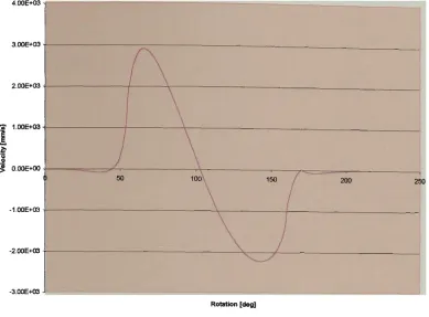
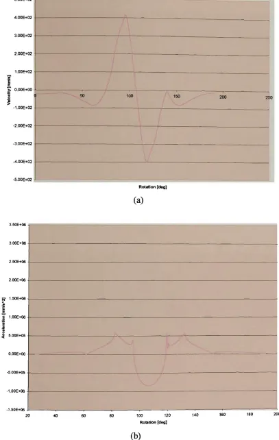
4.3 Simulation Results

Once the D V C model was complete, computer simulations were performed under

various operating conditions. The purpose was to determine the valve lifts, velocities,

acceleration and constraint forces generated in the D V C model. Each simulation was

for 1 second, with 50000 steps. The steps represent the total number of times output

information is provided over the entire simulation.

The engine speeds for the DVC simulation were 60 rpm, 3000 rpm, and 6000 rpm

The valve crank is a substitute for the camshaft and the camshaft rotates at half the

speed of the engine. The camshaft speeds are shown in Table 4.2.

Due to the fact there is rotational motion applied to the valve crank for it to drive the

model, these speeds were converted to degrees/sec using the equation below,

oo = RPM/60* 360 (4.1)

Engine Speed (rpm)

60

3000

6000

Camshaft Speed (rpm)

30

1500

3000 J

Speed (deg/sec}

180

9000

18000

4.3.1 D V C Valve Profile

The rotational location of the guideshaft determines the valve lift. The guideshaft,

which is connected to the engine management system via a hydraulic mechanism,

rotates according to the engine speed and load m u c h in the same manner as that

developed by Steinberg et al. (1998). The D V C system would use a hydraulic hub

connected to the guideshaft and the E C U would control the valves that supply oil to

the hydraulic hub. However, the D V C design would be simpler because it wouldn't

rotate like those connected to a continuously spinning camshaft. Using A D A M S , the

guideshaft w a s rotated to fixed positions in increments of 1 degree between minimum

lift and m a x i m u m lift.

As the guideshaft rotates clockwise, the valve lift increases and the valve lift

decreases w h e n the guideshaft rotates anti - clockwise. The guideshaft can rotate from

minimum lift to m a x i m u m lift in a span of 10 degrees. The valve lifts of the D V C

system are shown in Figures 4.24, 4.25, 4.26, 4.27, 4.28, 4.29, 4.30, 4.31, 4.32, 4.33

ZJ J<i

25 50 75 100 125 150

Valve Crank Rotation [deg] .T.T.T.T.T.T.T.T.T.T.T.T.T.TM

_1

i

4

a

Al

/ " \

\

\

/

I

\

25 50

-Guide 358d eg

75 100 125 150

Valve Crank Rotation [deg]

12.00

10.00

5 00

6.00

4 00

2.00

0.00

/ _\

1

1 \

-Guide 359deg

0 25 50 75 100 125 150 175 200 225

Valve Crank Rotation [deg]

i PiifTa'm.'v'MgiP—i

I A j | JinJete fie»ie« Ssftnoi I o * a«t>

^1

a

n

AJ

M

p y n m c

"3

r Dttbug Mof... | Rondo Icon* JLfUBl » 12.00 10.00 8.00 3 6.00 4.00 2.00 0.00

25 50

| Guide Odeg )

75 100 125 150

Valve Crank Rotation [deg]

10.00

8.00

5

6.00 | Guide 1deg [

4.00

2.00

0.00

25 50 75 100 125 150 175 200 225

Valve Crank Rotation [deg]

12.00 10.00

(00

4.00 2.00 0.00

-Guide 2deg |

1

n

IDynam

Sfixiatc B e v w w Setimos Iooh H o p - • —

Dynamo

1

[**• 3

r Debug Mae... |

Render I Icon j %

10.00

100

j 6.00

S

1

4.00

0.00

/ \

\

/ \

25 50 75 100 125 150 Valve Crank Rotation [deg]

175 200 225

12.00

10.00

too

5 6.00 -Guide 4deg

4.00

2.00

12.00

-?

a

> 5 >

4.00 2.00

-'

25 50

/ \ .

75 100 125 Valve Crank Rotation [deg]

150 175 200 27

— G u i d e 5deg j

5

12.00

10.00

8.00

6.00

2

4.00

-Guide 6deg |

2.00

0 . 0 0 ^

25 50 75 100 125

Valve Crank Rotation [deg]

_, OkfPJi u_j] /2

3

Aj

a

- ll S > ™ J - »

AJbm*

il

M i l

SirnJKiori

jsnaial

|D«fwrnc _*] 1 End im'-i

rr~

[si,,.,

roooo

W|

@ll

r Debug More | F k n d M | Icora j |

Bt

10.00

8.00

600 -Guide 7deg [

4.00

2.00

0.00

25 50 75 100 125 150

Valve Crank Rotation [deg]

175 200 225

Figures 4.24 to 4.34, s h o w the valve lifts from m a x i m u m lift in Figure 4.24 to almost

zero lift in Figure 4.34. T h e D V C system m o v e s the valve from a m a x i m u m lift of

10.70 m m to virtually zero lift in a span of 10 degrees rotation of the guideshaft.

M a x i m u m lift of 10.70 millimetres is achieved w h e n the guideshaft is positioned at

357 degrees (three degrees clockwise from start location), with the valve lift

decreasing at about one millimetre with every 1 degree rotation of the guideshaft. For

example, Figure 4.25 shows the valve lift w h e n the guideshaft is at 358 degrees, with

the lift being 9.73 m m , while Figure 4.26 shows the valve lift at 8.63 m m , w h e n the

guideshaft is positioned at 359 degrees. A s the guideshaft begins to rotate anti

-clockwise from the m a x i m u m valve lift position of 357 degrees, the valve lift

gradually decreases. T h e positions of the guideshaft as seen from Figures 4.24 to 4.34,

illustrate the different positions of the guideshaft and their subsequent effect o n the

valve lift. M i n i m u m lift is achieved w h e n the guideshaft is at 7 degrees, as seen in

Figure 4.34, the valve lift is 0.36 m m which is virtually zero.

This result confirms that due to the DVC system being able to achieve almost zero

valve lift, there is no need for the throttle, as the valves themselves can limit the

pressures in the cylinders and as a consequence, limit engine output. The most

important aspect that can be seen from the figures, is that the D V C system can

achieve a variation in lift, which means that any valve lift between zero to m a x i m u m

lift is quite attainable. Figure 4.35 illustrates the variable lift of the D V C system and

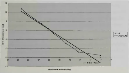
Figure 4.36 illustrates the m a x i m u m valve lift versus valve crank rotation. It can be

seen from Figure 4.36 that the relationship between m a x i m u m valve lift and valve

Figure 4.35 - Variable lift of D V C system

M a x i m u m Valve Lift versus Valve Crank Rotation