Crossing Minimization in k-layer graphs

(1)

ABSTRACT

GUPTA, SAURABH. Crossing Minimization in k-layer graphs. (Under the direction of Professor Matthias Stallmann).

The crossing minimization problem in graphs has been extensively studied for the case when graphs are to be embedded on two layers. There are many well known heuristics for the 2-layer crossing minimization problem, like, for example, the barycenter and the median heuristic. The problem has not been studied much for k-layer graphs. The k-layer graph crossing minimization problem has specific application in aesthetic design of hierarchical structures, in VLSI circuit design to reduce the total wire length and crosstalk, and in various organization charts, flow diagrams and large graphs that arise in activity-based management.

(2)

Crossing Minimization in k-layer Graphs by

Saurabh Gupta

A thesis submitted to the Graduate Faculty of North Carolina State University

in partial fulfillment of the requirements for the Degree of

Master of Science

Computer Science

Raleigh, North Carolina 2008

APPROVED BY:

Dr. Carla D. Savage Dr. Rada Chirkova

Dr. Matthias Stallmann

(3)

Dedication

To my parents. . .

(4)

Biography

Saurabh Gupta was born in Karnal, India. He did his under graduation from Punjab Engineering College, Chandigarh, India in the field of Electronics and Electrical Communication. After that, he worked for more than two years with Infosys Technologies Limited, Bangalore, India in the field of web application development.

(5)

Acknowledgements

I have been fortunate to have people who helped and inspired me while working on my thesis. I would like to acknowledge their contribution towards the completion of this thesis work.

First and foremost, I would like to thank my family, who has been very supportive all throughout my life. Their enormous faith in me has helped a lot in my confidence.

I would like to thank my thesis advisor Dr. Stallmann for his guidance and patience at times when it was needed the most. He was always keen to listen to my ideas and to suggest improvements. This thesis work would not have been possible without his inputs. His vast knowledge about the subject helped me enormously. His methodical approach towards work is an important lesson I learnt during this thesis work. I would also like to thank him for the software provided by him which has been used in this thesis work.

(6)

Table of Contents

List of Tables ...vii

List of Figures ...viii

Chapter 1. Introduction ... 1

Chapter 2. Literature Survey ... 5

2.1 Overview of the work done ... 5

2.2 Heuristics in bi-layer graphs ... 6

2.3 Work done in the case of k-layer graphs ... 9

2.4 Testing ... 10

Chapter 3. Description of Heuristics ... 12

3.1 Introduction ... 12

3.2 Initial Ordering ... 12

3.3 Order of selection of layers ... 12

3.4 Heuristics Used for sorting ... 14

3.5 Use of neighboring layers ... 15

3.6 Heuristics Implemented ... 15

Chapter 4. Experimental set up ... 30

4.1 Trees ... 30

4.2 Direct Acyclic Graphs (dags) ... 32

4.2.1 Types of dags ... 32

Equal layer dag ... 32

Unequal Layer dag ... 33

4.3 Performance criteria ... 33

Chapter 5. Results ... 35

5.1 Initial Results ... 35

5.2 Names Used for Heuristics... 37

5.3 Results of experiments performed over a random class of tress ... 38

5.3.1 Bary vs. Mod-bary ... 38

5.3.2 Mod-bary vs. Mod-median ... 40

5.3.3 Modified Weighted Edge Length vs. Traditional Heuristics ... 40

5.3.4 Mod-bary vs. Maximum Crossings Node ... 41

5.3.5 Performance of MCN with iterations... 43

5.3.6 Effect of number of layers on minimum crossings iteration for MCN ... 46

5.3.7 Effect of depth first search (dfs) implementation for initial ordering on all heuristics ... 46

5.3.8 Performance of MCN + dfs with iterations ... 48

5.3.9 MCN vs. mod-bary treated graph ... 52

5.3.10 Performance of MCN with larger graphs ... 52

5.3.11 Consistency of Heuristics ... 54

5.4 Results of experiments performed over dags ... 55

(7)

5.4.2 Mod-bary vs. Mod-median ... 55

5.4.3 Modified Weighted Edge Length vs. Traditional Heuristics ... 56

5.4.4 Mod-bary vs. Maximum Crossings Node ... 57

5.4.5 Effect of edge density on heuristics performance ... 59

5.4.6 A Mixed Heuristic ... 59

5.4.7 Mixed Heuristic vs. Mod-bary and MCN ... 60

5.4.8 Performance of chosen heuristics over larger graphs ... 60

5.4.9 Performance of mixed heuristic over iterations ... 61

5.4.10 Consistency of Heuristics ... 64

5.5 Comparison of performance of heuristics on dags as dense as trees ... 64

Chapter 6. Conclusions and Future Work ... 67

Bibliography ... ... ..69

Appendix ... ... ..72

Representation of Graph Properties ... ..73

Dot files... 73

Ord files ... 73

Isomorphism classes ... 73

(8)

List of Tables

Table 3.1 Table of Heuristics ... 28

Table 5.1 All Heuristics performance on trees ... 35

Table 5.2 All heuristics performance on dags ... 36

Table 5.3 Bary and Mod-bary performance on trees ... 38

Table 5.4 Mod-bary vs. Mod-median on trees... 40

Table 5.5 Mod-WEL vs. traditional heuristics on trees ... 41

Table 5.6 Mod-bary vs. MCN on trees ... 41

Table 5.7 MCN with iterations ... 43

Table 5.8 Minimum crossings iteration with layers for MCN ... 46

Table 5.9 Affect of dfs ... 47

Table 5.10 Graphs with dfs + MCN iterations ... 48

Table 5.11 MCN performance with increase in nodes ... 53

Table 5.12 Heuristics performance with isomorphism class ... 54

Table 5.13 Bary vs. Mod-bary on dags ... 55

Table 5.14 Mod-bary vs. Mod-median on a daag ... 56

Table 5.15 Mod-WEL vs. traditional heuristics on dags ... 56

Table 5.16 Mod-bary vs. MCN on dags ... 57

Table 5.17 Mixed heuristic vs. Mod-bary and MCN on dag ... 60

Table 5.18 Performance of Mod-bary, MCN and mixed-heuristic on large dags ... 61

Table 5.19 Performance of mixed-heuristics over iterations ... 61

Table 5.20 Performance of MCN, Mod-bary and mixed-heuristic on isomorphism class of dags ... 64

(9)

List of Figures

Figure 1.1 An unsorted 3-layer graph ... 2

Figure 1.2 A sorted 3-layer graph ... 2

Figure 2.1 A 2-layer graph with top layer fixed and bottom layer barycenter weights calculated ... 7

Figure 2.2 The 2-layer graph after the bottom layer has been sorted according to barycenter ... 7

Figure 2.3 A 2-layer graph with top layer fixed and bottom layer median weights calculated ... 8

Figure 2.4 The 2-layer graph after the bottom layer has been sorted according to median heuristic ... 8

Figure 3.1 The original 5-layer graph with 23 nodes. First stage of up sweep of simple barycenter heuristic. ... 16

Figure 3.2 Second stage of up sweep of simple barycenter heuristic. ... 16

Figure 3.3 Third stage of up sweep of simple barycenter heuristic. ... 17

Figure 3.4 Fourth stage of up sweep of simple barycenter heuristic. ... 17

Figure 3.5 Fifth stage of up sweep of simple barycenter heuristic. ... 18

Figure 3.6 First stage of modified barycenter heuristic. ... 19

Figure 3.7 Second stage of modified barycenter heuristic. ... 19

Figure 3.8 Third stage of modified barycenter heuristic. ... 20

Figure 3.9 Fourth stage of modified barycenter heuristic. ... 20

Figure 3.10 Fifth stage of modified barycenter heuristic... 21

Figure 3.11 Sixth stage of modified barycenter heuristic. ... 21

Figure 3.12 The original 5-layer graph with 23 nodes ... 23

Figure 3.13 Second stage of modified weighted edge length heuristic. ... 23

Figure 3.14 Third stage of modified weighted edge length heuristic. ... 24

Figure 3.15 Fourth stage of modified weighted edge length heuristic. ... 24

Figure 3.16 Fifth stage of modified weighted edge length heuristic. ... 25

Figure 3.17 Sixth stage of modified weighted edge length heuristic. ... 25

Figure 3.18 First stage of maximum crossings node heuristic. ... 26

Figure 3.19 Second stage of maximum crossings node heuristic. ... 26

Figure 3.20 Third stage of maximum crossings node heuristic. ... 27

Figure 3.21 Fourth stage of maximum crossings node heuristic. ... 27

Figure 3.22 Fifth stage of maximum crossings node heuristic. ... 28

Figure 4.1 is a tree with 100 nodes, 7 layers and Aspect Ratio of 1 (Dense and more number of crossings) ... 31

Figure 4.2 is a tree with 100 nodes, 7 layers and Aspect Ratio of 128 (Sparse and lesser number of crossings) ... 31

Figure 4.3 is an equal layer dag with 20 nodes, 5 layers and edge density of 1.5 ... 32

Figure 4.4 is an unequal layer dag with 20 nodes, 4 layers and edge density of 1 ... 33

Figure 5.1 Simple Barycenter applied to a tree ... 39

(10)

Figure 5.3 MCN applied to a tree ... 42

Figure 5.4 Modified barycenter applied to a tree ... 43

Figure 5.5 8 iterations of MCN applied to a tree ... 44

Figure 5.9 Difference in crossings minimization of the heuristics due to dfs ... 47

Figure 5.10 Dfs applied to a tree... 49

Figure 5.11 Dfs and 8 iterations of MCN applied to a tree ... 50

Figure 5.15 Performance of MCN with iterations ... 52

Figure 5.16 MCN applied to a dag ... 58

Figure 5.17 Mod-bary applied to a dag... 58

Figure 5.18 Performance of heuristics for various edge densities ... 59

Figure 5.19 Mod-bary applied to a dag... 62

Figure 5.20 Mod-bary and 32 iterations of MCN applied to a dag ... 62

(11)

Chapter 1. Introduction

This chapter introduces the crossing minimization problem in k-layer graphs and its significance. We present notation and graph terminology relevant to the remaining part of this thesis work, and give a formal definition of the problem of minimizing crossings in a k-layer graph.

A k-layer embedding of a k-partite graph is one in which all its vertices are placed on k horizontal lines, one horizontal line for each partition of the graph. More specifically, a k-layer embedding puts vertices V0, V1, V2, V3..., Vk-1 (the k partitions) on k parallel lines, with

vertices of Vi on the line y = i. The layers are numbered from the lowermost layer to the

uppermost. Since it is k-partite the graph has edges between vertices on adjacent layers only and these are represented as straight lines. Because a k-layer embedding implies a k-partite graph, we simply refer to k-layer graphs from here on.

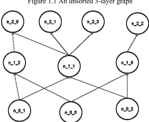
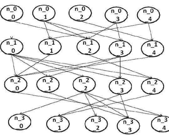
Observe that the permutation of vertices on each layer determines the number of crossings. Figure 1.1 shows a 10 node, 3 layer directed graph with the vertices on each layer permuted in some random order. Figure 1.2 shows the same graph with the vertices on each layer sorted so as to reduce its crossings. The reader can verify that this ordering produces the minimum number of crossings.

This thesis deals with reducing the number of crossings in a k-layer graph. A graph with no crossings is called a k-planar graph. The crossings problem has been proved to be NP complete problem even for a 2-layer graph when one of the layers is kept fixed. [GJ83] Given a graph G, for crossings minimization problem, the requirement is to place its vertices in such an order so that the crossings in the graph are minimized. The problem is of specific interest in

(12)

Figure 1.1 An unsorted 3-layer graph

Figure 1.2 A sorted 3-layer graph

(ii)Entity relationship diagrams or any flow diagrams. [T96]

(iii) Reducing the wiring congestion and cross talk in VLSI circuits, which further helps to reduce the total wire length and the total layout area.[CLR87, MS95]

(iv) Organization charts [D94].

A 3-layer, 10 nodes graph with initial number of crossings = 11 when no heuristic is applied to it

(13)

(v) In large graphs generated in activity based management for tracking flows of products and services. [WBSDRRP08]

For any graph G with k layers, its vertex set on layer 0, 1, 2, 3..., k-1 is denoted by V0,

V1, V2, V3..., Vk-1. The edge set of the graph is denoted by E, where

E ⊆ (V0 x V1) ∪ (V1 x V2) ∪ (V2 x V3)………∪ (Vk-2 x Vk-1).

The number of vertices in a layer i is denoted by si.

Let the graph G given by G = (V0, V1, V2, V3..., Vk-1) be a k-partite graph with

vertex set V0∪V1∪ V2∪……Vk-1 and edge set

E ⊆ (V0 x V1) ∪ (V1 x V2) ∪ (V2 x V3)………∪ (Vk-2 x Vk-1).

The problem is to minimize the number of crossings in the graph, i.e., if crossings in graph is given by

Crossings = C (G, ∏0, ∏1, ∏2..., ∏k-1 )

where ∏i is the permutation of vertices in the layer i where i varies from 0 to k-1. A crossing in a graph occurs, when for e.g., if there are nodes a and b on layer i and nodes c and d on layer i+1 with edges ac and bd with order(a) < order(b), while order(c) > order(d).

The problem definition is then to

Minimize (Crossings)

and the solution to the problem consists of finding the permutations ∏0, ∏1, ∏2..., ∏k-1 on the

layers which lead to minimum crossings.

(14)

Thus our thesis work consists of (i) study of various heuristics of 2-layer graphs and finding the best ones among them; (ii) using different flavors of those heuristics to find their best implementations for k-layer graph crossing minimization problem; (iii) testing those heuristics on a varied and large sample of graph families to test their performance across different graphs; (iv) testing the consistency in the performance of the proposed heuristics on the same graph family; (v) suggesting future work for the k-layer graph crossings minimization problem

(15)

Chapter 2. Literature Survey

The chapter discusses the initial work done in crossing minimization problem and the need to find a solution to the problem (Section 2.1). Section 2.2 explains two good heuristics in case of 2-layer graph crossing minimization problem – barycenter and median. Section 2.3 talks about sifting heuristic, a heuristic which was proposed for k-layer crossing minimization problem. The experimental set up that has been used earlier to test new heuristics is discussed in Section 2.4.

2.1 Overview of the work done

Work in the field of crossing minimization was done as a part of solving the bigger problem – improving the readability of hierarchical structures. Warfield in his paper [W77] proposed a way to deal with a combinatorial problem of crossing minimization. Sugiyama et al. [STT81] proposed an approach, now referred to as the Sugiyama approach to obtain aesthetically pleasing drawings of hierarchies and other graphs. The steps they proposed are as follows

i) First, a proper hierarchy of vertices is formed from the given set of directed pair wise relations. Dummy vertices are introduced to remove any long edges.

ii) Crossings of edges are reduced.

iii) Horizontal positions of vertices are determined.

iv) A two dimensional picture of hierarchical structure is drawn by removing the dummy vertices and regenerating the long edges.

(16)

even in the fixed-layer problem, for a 2-layer graph, it is NP hard to compute the minimum crossings in the graph. Major work done in crossing minimization problem has been on 2-layer graphs and most of that work has been theoretical [W77, STT81, MSM01, D94, C95, EK86, SBG99] but there is some experimental work as well. [SBG01, JM04] In this thesis, an attempt has been made to extend this problem further to find solutions to crossing minimization problem in the case of k-layer graphs, and propose heuristics that deals with the crossing minimization problem as a fixed-layer problem and follow a layer by layer approach.

Initial study for the problem of k-layer graph involves generalizing the heuristics that have been used for 2-layer graphs, whether or not they perform well in the case of 2-layers [STT81, D94, C95, EK86]. Later, a few variants of the old heuristics [STT81, D94, MSM01] are applied and tested for k-layer graphs. Some work have been done in case of k-layer graphs too which helped to know which heuristics have already failed.

2.2 Heuristics in bi-layer graphs

Among the earlier works was the work done by Warfield, which was used and extended by Sugiyama et al. in [STT81] to find the solution to problem having more than five vertices in a layer. Sugiyama et al. [STT81] proposed two algorithms for 2-layer graphs. The first one is the barycenter in which they used generating matrix defined by Warfield to define their own matrix, called as barycenter-ordered generating matrix. It is a two phased algorithm. This algorithm is extensively used even now in the case of 2-layer graphs and is used in this thesis work in more than one heuristic. The other method proposed is the Penalty Minimization method in which they consider the problem of crossing minimization as the problem to determine the set of orders in all the two-combinations of vertices.

(17)

decrease the crossings. This is done continuously with alternating layers. Methods which have proved efficient in 2-layer graphs and their variants are used in this thesis work. Throughput this thesis work the term vertices and nodes will be used interchangeably.

The two most common heuristics are the barycenter and median heuristics. Both of them are known as ‘averaging heuristics’, since they compute the positions of nodes based on the average position of their adjacencies on the other layer. A brief explanation of the heuristics is given below.

• Barycenter: In the barycenter heuristic, the nodes in a layer are sorted with respect to

the position of their adjacencies. The mean of the positions is calculated and the nodes are sorted in increasing order of their means. For more details see [STT81]. Figures 2.1 and 2.2 demonstrate a small example of barycenter heuristic.

Figure 2.1 A 2-layer graph with top layer fixed and bottom layer barycenter weights calculated

(18)

• Median: In the median heuristic, the nodes are sorted with respect to the median of

their adjacencies instead of mean. For more details see [EW94]. Figures 2.3 and 2.4 demonstrate a small example of median heuristic.

Figure 2.3 A 2-layer graph with top layer fixed and bottom layer median weights calculated

Figure 2.4 The 2-layer graph after the bottom layer has been sorted according to median heuristic

There are few more heuristics for the 2-layer problem in which the permutation of nodes on both layers takes place simultaneously. These include the stochastic heuristic [D94], the greedy insert heuristic [EK86], the greedy switch heuristic [EK86], the split heuristic [EK86] and the assign heuristic [C95]. In another approach to solve this problem, Junger and Mutzel [JM04] transformed the problem into an integer programming problem and subsequently solved it using the branch and cut method.

(19)

insert and assignment heuristic performed well in case of dense graphs, they observed that the most interesting graphs for practical applications are sparse graphs, in which each node has an average in degree of two. For more details about their experiments and procedure see [JM04].

Stallmann et al. [SBG01] proposed a new heuristic – adaptive insertion which uses the concept of local search to improve solutions. The adaptive insertion heuristic was modified in reaction to preliminary experimental results before taking the final form reported in [SBG01]. The heuristic consists of inserting each node of a given layer in the position that would lead to fewest crossings and then fixing the position of that node and its immediate neighbor to the left. All the nodes are similarly repositioned. The experiments performed led the authors of the paper to conclude that even though the heuristic performs well, it requires a large number of passes and the number of passes required to obtain good solutions increases non-linearly with the number of edges.

The authors of [SBG01] also experimented with a heuristic that combines adaptive insertion with barycenter to obtain more good results than using adaptive insertion alone. They also preceded other heuristics with an initial placement. Two initial placement strategies were proposed based on the concept of breadth first search.

A novel aspect of the instances on which heuristics were tested in [SBG01] was the use of random and isomorphism classes of graphs to be described and used later in our experiments for this thesis work.

2.3 Work done in the case of k-layer graphs

(20)

The authors considered three entirely different criteria for choosing the next vertex v to sift

1. The vertices are considered in their preassigned vertex order in the layer, for e.g., from left to right.

2. The vertices of the whole graph are sorted by their in degree and sifted in that order regardless of layer.

3. The vertices are chosen on a completely random basis.

Experiments were done comparing the sifting criteria and comparing sifting with the traditional median and barycenter heuristics.

The experiments were conducted on sparse graphs, having ∑vi edges, where vi is the

number of vertices on layer i for i = 1 to k. So, on an average a vertex had an in-degree of 2. The test instances chosen had a maximum of 12 layers and an average of 10 nodes per layer.

Matuszewski et al. demonstrated that all three variations of their sifting heuristic produces better results than the traditional barycenter and median sweep approach for the graphs on which they tested the heuristics.

2.4 Testing

Stallmann et al. [SBG01] in testing of various heuristics proposed the idea of testing them on a wide range of random and isomorphism classes. A random class of graphs consists of some number of graphs (usually 32, 64 or 128), generated in such a way that all instances in the class have the same number of nodes and edges and the graphs are sometimes similar in other ways as well. An isomorphism class consists of graphs which are random presentations of the same graph G. The name isomorphism derives from the fact that every graph in an isomorphism class is isomorphic to every other graph. The graph differ only in (a) the order of appearance of the edges in the input file, and (b) the initial order of nodes on each layer as specified by an auxiliary ordering file.

(21)

when presented with the same input, and only the initial order of nodes is arranged differently. Both types of classes are used in the experiments conducted for this thesis work.

Most experimental work on crossing minimization problem considers the effects of density, which is number of edges divided by number of nodes that leads to the concept of sparse and dense graphs, for testing the performance of heuristics. The work of [SBG01] is not different nor is the work reported in this thesis.

(22)

Chapter 3. Description of Heuristics

New heuristics are proposed in this chapter for crossing minimization problem in k-layer graphs. Section 3.1 gives a brief overview about design issues of heuristics for k-k-layer graphs. Section 3.2, 3.3 and 3.4 discusses design aspects of heuristics which leads to twenty five different heuristics. Section 3.5 discusses the chosen heuristics which are found to work well after an initial set of experiments, and a couple of traditional heuristics.

3.1 Introduction

The heuristics for crossing minimization on a k-layer graph, differ from each other in one or more of the following aspects –

i) Initial ordering of the nodes

ii) Order in which the layers are considered for sorting of nodes iii) Heuristic used to sort the nodes in a layer.

iv) Use of neighboring layers.

For 2-layer graphs, only the initial ordering and the sorting heuristic are relevant. The layer order switches back and forth between the two layers and the only neighboring layer to consider is the other layer. There are wider options available in k-layer graphs, which make for a much richer selection of possible heuristics.

3.2 Initial Ordering

Two types of initial ordering of nodes are followed in this thesis work. One is the random initial ordering while the other one uses depth first search (dfs) for initial ordering of the nodes.

3.3 Order of selection of layers

(23)

• Sequential Sweep: An iteration of the heuristic consists of one up sweep and one down

sweep. The up sweep starts from layer 1 and goes till layerk–1 while the down sweep

starts from layer k and goes till layer 2.

• Maximum Crossings Node: An iteration of the heuristic consists of finding the node

with the maximum number of crossings, and choosing the layer of that node. This node is not considered again in future iterations until all the nodes of the graph have been considered once.

• Maximum Crossings Layer: An iteration of the heuristic consists of choosing the layer

with the maximum number of crossings, whose order remains fixed in the remaining part of that iteration. The number of crossings is recomputed after each layer is reordered. After the first layer is reordered, the layer with the second largest number of crossings is chosen. This process is continued till all the layers are considered once.

• Maximum Crossings Layer, Variation 1: An iteration of the heuristic, like that of the

maximum crossings layer heuristic, chooses the layer with maximum number of crossings and keeps it fixed in the remaining part of the iteration. Let this layer be l. First this layer is sorted, and then the layers above to it are sorted, i.e., from layer l+1 to k-1. Then the layers below, i.e., layers l–1 to 2 are sorted.

• Maximum Crossings Layer, Variation 2: This is a subtle variation of the maximum

(24)

3.4 Heuristics Used for sorting

In addition to the earlier heuristics used for 2-layer graphs, i.e., barycenter and median, a couple of new heuristics for sorting nodes in a given layer are used in this thesis work. These are –

• Edge Length and Weighted Edge Length: In the heuristic, each node x is associated

with a weight w(x). In every layer, first the total weight of a node is calculated, which is then used for it’s sorting in that layer. Nodes are arranged from left to right in the increasing order of their weight.

Let the node be x and p(x) be the position of that node in its layer.

Let us assume that this node has edges with nodes y1, y2, y3 …. yq in its adjacent layer.

Let p(y1), p(y2), p(y3) … p(yq) be the position of the nodes y1, y2, y3 …. yq in their layer.

Let c1, c2, c3………cq be the crossings contributed by the edges xy1, xy2, xy3… xyq

respectively.

The weight of a node x is given by Weight w(x) = p(x) + f(x), where

f(x) = ( p(y1) - p(x)) + ( p(y2) - p(x))+ ( p(y3) - p(x)) ……. + ( p(yq) - p(x))

for the edge length heuristic, and

f(x) = c1( p(y1) - p(x)) + c2( p(y2) - p(x))+ c3( p(y3) - p(x)) ……. + cq( p(yq) - p(x))

for the weighted edge length heuristic

Nodes on a layer are sorted by increasing weight w(x). The heuristic is based on the assumption that by reducing the length of edges, their probability of contributing crossings in the graph can be reduced. The idea is thus to place the nodes closer to their adjacent nodes in other layers which leads to a reduction in edge length. A further improvement is to prioritize the edges, based on the number of crossings they contribute in the graph which leads to the concept of weighted edge length heuristic.

• Middle sorted Edge Length and Middle sorted Weighted Edge Length: The weight of

(25)

the node with next largest weight to the right of first node, the next to the left of first node. As nodes are considered in order of decreasing weights, they are alternately placed to the right or left of the nodes that have already been placed.

• Sifting heuristic: The node is moved to a position within its layer that minimizes the

crossings caused by it. Here the chosen node will always be the one with maximum number of crossings, unlike how the nodes were chosen in [MSM99].

3.5 Use of neighboring layers

A k-layer graph unlike a 2-layer graph has nodes which have adjacencies both on layer above and on layer below. Thus it is possible to sort a layer based on the layer above it or layer below it or based on both the layers. We refer to these variations as upward orientation,

downward orientation and bi directional orientation. They are as follows:

• Upward orientation: The nodes are sorted with respect to their adjacencies on the layer

above it.

• Downward orientation: The nodes are sorted with respect to their adjacencies on the

layer below it.

• Bi directional orientation: The nodes are sorted with respect to their adjacencies both

on the layer above and layer below it.

3.6 Heuristics Implemented

Twenty five heuristics were implemented initially. After some initial tests, only six of them are selected for future experiments. The selected heuristics are:

• Simple Barycenter: This is the traditional barycenter heuristic used in literature

[STT81]. It uses sequential sweep, barycenter heuristic and upward orientation for up sweep and downward orientation for down sweep.

(26)

Figure 3.1 The original 5-layer graph with 23 nodes. First stage of up sweep of simple barycenter heuristic.

Figure 3.2 Second stage of up sweep of simple barycenter heuristic. The upsweep starts from lowermost layer. The barycenter weights of the lower layer nodes are calculated.

(27)

Figure 3.3 Third stage of up sweep of simple barycenter heuristic.

Figure 3.4 Fourth stage of up sweep of simple barycenter heuristic.

The second layer is now sorted w.r.t its barycenter weights calculated in previous figure. The barycenter weights of third layer nodes are now calculated.

(28)

Figure 3.5 Fifth stage of up sweep of simple barycenter heuristic.

• Simple Median: This is the traditional median heuristic used in literature [EW94]. It

uses sequential sweep, the median heuristic for sorting, and upward orientation for up sweep, downward orientation for down sweep.

• Modified Barycenter: This uses Maximum Crossings Layer order and barycenter

heuristic. It uses bi direction orientation for chosen layer everytime.

The figures 3.6-3.11 illustrate an iteration of the heuristic. Again, the figures show the calculated weights of nodes and the sorted nodes at different stages of the iteration –

(29)

Figure 3.6 First stage of modified barycenter heuristic.

Figure 3.7 Second stage of modified barycenter heuristic. The maximum crossings layer is determined which in this case is layer four. The barycenter weights of the nodes in this layer are calculated considering the adjacent nodes in both its upper and lower layer.

(30)

Figure 3.8 Third stage of modified barycenter heuristic.

Figure 3.9 Fourth stage of modified barycenter heuristic.

The nodes in layer five are sorted w.r.t its barycenter weights calculated in previous figure. The barycenter weights of layer below maximum crossings layer i.e. layer three are now calculated.

(31)

Figure 3.10 Fifth stage of modified barycenter heuristic.

Figure 3.11 Sixth stage of modified barycenter heuristic.

The nodes in layer two are sorted w.r.t its barycenter weights calculated in previous figure. The barycenter weights of layer one are now calculated.

(32)

• Modified Median: This uses Maximum Crossings Layer order and median heuristic for

sorting. It uses bi direction orientation for chosen layer and then downward orientation for layers above it and upward orientation for layers below it.

• Modified Weighted Edge Length: This uses Maximum Crossings Layer Variation 1

and weighted edge length heuristic for sorting. It uses bi direction orientation for chosen layer and then downward orientation for layers above it and upward orientation for layers below it.

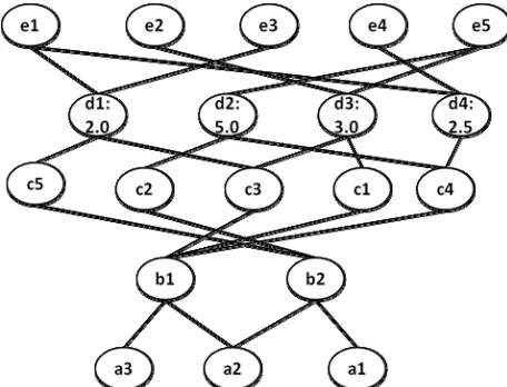
The heuristic involves calculating the weight of all the nodes in the graph. Let us consider the graph in figures 3.12 - 3.17. The maximum crossings layer in this graph is layer 4 involving nodes d1, d2, d3 and d4. As an example, the total weight of node d1

is calculated below considering its adjacencies both with the layer above it (e1, e3) and

the layer below it (c3, c5).

For node d1the total weight is calculated as:

weight(d1) = p(d1) + f(d1)

p(d1) = 1

f(d1) = crossings by edge d1e1{p(e1) – p(d1)} + crossings by edge d1e3{p(e3) – p(d1)} +

crossings by edge d1c3{p(c3) – p(d1)} + crossings by edge d1c5{p(c5) – p(d1)}

p(e1) = 1, p(e3) = 3, p(c3) = 3 and p(c5) = 5

for the present state of graph

f(d1) = 0*{1–1} + 2*{3–1} + 2*{3–1} + 5*{5–1}

= 28

Thus, w(d1) = 1 + 28

Weight w(d1) = 29

The figures 3.12 - 3.17 illustrate an iteration of weighted edge length. The

(33)

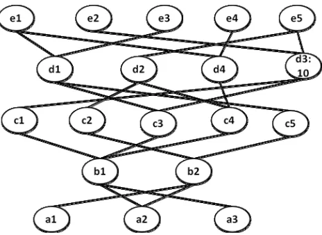
Figure 3.12 The original 5-layer graph with 23 nodes First stage of modified weighted edge length heuristic.

Figure 3.13 Second stage of modified weighted edge length heuristic. The maximum crossings layer is layer four. The weighted edge length weights of the nodes of layer four are calculated.

(34)

Figure 3.14 Third stage of modified weighted edge length heuristic.

Figure 3.15 Fourth stage of modified weighted edge length heuristic. The nodes in the layer five are sorted w.r.t. weighted edge length weights calculated in previous figure. Now, the weight of nodes of layer below to maximum crossings layer which is layer three is calculated.

(35)

Figure 3.16 Fifth stage of modified weighted edge length heuristic.

Figure 3.17 Sixth stage of modified weighted edge length heuristic. The nodes in the layer two are sorted w.r.t. weighted edge length weights calculated in previous figure. Now, the weight of nodes of layer one is calculated.

(36)

• Maximum Crossings Node: This uses Maximum crossings node order and sifting

heuristic for sorting.

The figures 3.18 – 3.22 illustrate an iteration of the heuristic. The figures show the calculated crossings of maximum crossings node at different positions in the layer and it sorted position in its layer after the iteration of the heuristic –

Figure 3.18 First stage of maximum crossings node heuristic.

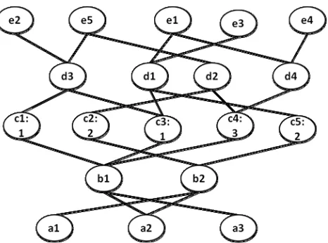
Figure 3.19 Second stage of maximum crossings node heuristic. The crossings of all the nodes in the graphs are calculated to determine the maximum crossings node, which in this case is d3

The crossings of node d3 at first position in its layer is calculated.

(37)

Figure 3.20 Third stage of maximum crossings node heuristic.

Figure 3.21 Fourth stage of maximum crossings node heuristic. The crossings of node d3 at second position in its layer is calculated.

It is 8.

The crossings of node d3 at fourth and last position in its layer is

(38)

Figure 3.22 Fifth stage of maximum crossings node heuristic.

Most of the heuristics obtained by variations of the design aspects discussed earlier in the chapter are not competitive based on results of preliminary experiments. The heuristics which are eliminated early in the experiments conducted are listed in Table 3.1 for the sake of completeness. Recall that the orientation is determined by the order in which layers are considered.

Table 3.1 Table of Heuristics

Heuristic Name Order Used Heuristic Used

Edge Length Sequential Sweep Sorting Edge Length

Modified Barycenter v. 1 Maximum Crossings

Layer Variation 1 Barycenter

Modified Median v. 1 Maximum Crossings

Layer Variation 1 Median

Modified Edge Length v. 1 Maximum Crossings

Layer Variation 1 Edge Length

Weighted Edge Length Sequential Sweep Weighted Edge Length

Layer

Edge Length

Modified Weighted Edge Length v. 1

Maximum Crossings Layer

Weighted Edge Length

Modified Barycenter v. 2 Maximum Crossings

Layer Variation 2

Barycenter The node d3 is assigned the position of minimum crossings i.e.

(39)

Table 3.1 continued

Modified Median v. 2 Maximum Crossings

Layer Variation 2

Median

Layer Variation 2 Edge Length

Modified Weighted Edge Length

v. 2 Maximum Crossings Layer Variation 2 Weighted Edge Length

Modified Edge Length v. 3 Sequential Sweep Middle sorted Edge

Length

Layer Variation 1

Middle sorted Edge Length

Sequential Sweep Middle sorted

Weighted Edge Length Modified Weighted Edge Length

v. 4

Maximum Crossings Layer Variation 1

Middle sorted

Layer Middle sorted Edge Length

Maximum Crossings Layer

Middle sorted

Layer Variation 2

Middle sorted Edge Length

Maximum Crossings Layer Variation 2

Middle sorted

Thus, new heuristics were proposed in this section for solving crossing minimization problem in k-layer graphs. The four chosen heuristics and the two traditional heuristics which were discussed in this section are –

i) Simple Median

ii) Simple Median

iii) Modified Barycenter

iv) Modified Median

v) Modified Weighted Edge Length

(40)

Chapter 4. Experimental set up

To check the performance and consistency of the heuristics, they are tested over a wide range of graphs, by varying some of the parameters of the graph and observing the response of the heuristics in each case. The type of graphs which are chosen to test the heuristics are the trees and directed acyclic graphs (dags). The work in this thesis concentrates on the crossing minimization problem of hierarchical structures, thus in all the graphs discussed, the nodes have been properly assigned to different layers (assumed k in this thesis) and there are no long edges, i.e., the edges are only between the nodes of adjacent layers. In dags the default direction of edges is from lower to higher layers. More detailed discussion about the two types of graphs is done below.

4.1 Trees

The trees used in this thesis work are minimum spanning tree rooted on points chosen from a square. The number of nodes and layers in the tree are defined by the user. For a k layer tree, while traversing the nodes in the tree, the nodes are assigned layers labeled from layer 0 to layer k-1 first and then switching back the directions to go back to layer 0. The aspect ratio of tree determines how thick or sparse it is. A tree with a low aspect ratio is thick and has more crossings while a tree with large aspect ratio has long paths and has lesser number of crossings. Different attributes of the trees are varied individually, keeping all others constant to measure and observe the behavior of heuristics over various attributes of tree graphs. The attributes which are varied are the number of nodes, number of layers and aspect ratio of the tree.

(41)

Figure 4.1is a tree with 100 nodes, 7 layers and Aspect Ratio of 1 (Dense and more number of crossings)

(42)

4.2 Direct Acyclic Graphs (dags)

The second class of graph on which the heuristics are tested is the Directed Acyclic Graphs (dags). The dags are created with any number of nodes and layers, and user can assign nodes in each layer. The density of dags is also controlled by user. The dags which we used for testing in this thesis work have some special properties to be discussed later in this section.

4.2.1 Types of dags

The directed acyclic graphs tested are both equal layer and unequal layer. The dags are generated according to the rule -

i)Every node has at least one incoming edge

ii)Since the nodes in first layer will have no incoming edges, so all the nodes in layer one which do not have any outgoing edges too are removed from the dag.

Equal layer dag

In these dags, the number of nodes is almost constant in every layer. If s1, s2 ….

sk are the number of nodes in layers 1,2…k respectively, then

s1 ≈ s2≈…………≈ sk

A typical equal layer dag is shown in figure 4.3

(43)

Unequal Layer dag

In these dags, the number of nodes varies in each layer. The experiments are conducted on a class of symmetrically asymmetrical graphs in which the number of nodes in second layer is twice that in first layer, and also twice of that in third layer.

Alternatively, if s1, s2, s3, s4 …. sk are the number of nodes in layers 1, 2, 3,

4…k respectively, then

2s1 ≈ s2≈ 2s3 ≈ s4 ≈…………≈ 2sk-1≈ sk

A typical unequal layer dag is shown in figure 4.4

Figure 4.4 is an unequal layer dag with 20 nodes, 4 layers and edge density of 1

Several attributes of the dags are changed like number of nodes per layer, number of layers and also the edge density keeping other parameters constant and the performance of the heuristics is observed.

4.3 Performance criteria

(44)

of the heuristic. The number of iterations required to reach the minimum crossings value is also measured to check how quickly the heuristic reaches the desired result.

(45)

Chapter 5. Results

First, experiments are conducted with all the twenty five heuristics on a set of trees and dags to find the best performing heuristics. All the remaining experiments are then performed using the chosen heuristics. A couple of traditional heuristics are also included in the set to measure the relative performance of the chosen heuristics. The chosen heuristics are compared for their performances on trees and dags to determine the best heuristic among the chosen set. The iteration wise performance of the best or close to best heuristic is studied. The heuristics performance is also checked on larger graphs. In case of trees, the affect of initial ordering by depth first search is observed. While in the case of dags, a mixed heuristic is proposed and its performance is measured. Finally, the consistency of heuristics is tested by running them on an isomorphism class of 32 graphs.

5.1 Initial Results

Both Table 5.1 and Table 5.2 contain results of initial experiments conducted on trees and equal layer dags. The initial experiments are conducted to eliminate the heuristics which didn’t perform well or didn’t look interesting enough for future experiments.

Table 5.1 All Heuristics performance on trees

Heuristics Initial Crossings

Mean of Crossings

% of Initial crossings

Simple Barycenter 7595.5 6465.8 85.1

Simple Median 7595.5 6556.6 86.3

Edge Length 7595.5 6943.3 91.4

Modified Barycenter v. 1 7595.5 1442.6 19.0

Modified Median v. 1 7595.5 1497.9 19.7

Modified Edge Length v. 1 7595.5 1313.7 17.3

Weighted Edge Length 7595.5 7595.5 100

Modified Weighted Edge Length 7595.5 3144.3 41.4

Maximum Crossings Node 7595.5 1054.2 13.9

Modified Barycenter 7595.5 926.1 12.2

(46)

Table 5.1 continued

Modified Weighted Edge Length v. 1 7595.5 3370.6 44.4

Modified Edge Length v. 4 7595.5 7063 93.0

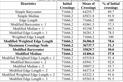
Table 5.2 All heuristics performance on dags

Heuristics Initial Crossings

Mean of Crossings

% of Initial crossings

Simple Barycenter 71666.2 64255.7 89.7

Simple Median 71666.2 65831.8 91.9

Edge Length 71666.2 71666.2 100

Weighted Edge Length 71666.2 71666.2 100

Modified Weighted Edge Length 71666.2 56306.8 78.6 Maximum Crossings Node 71666.2 36737.7 51.3

Modified Barycenter 71666.2 35829.7 50.0

Modified Median 71666.2 41406.6 57.8

(47)

Table 5.2 continued

After the experiments conducted, following heuristics are chosen for future experiments – 1) Two traditional heuristics, i.e., simple barycenter and simple median.

2) Two most best heuristics which are Maximum crossings node and modified barycenter. 3) The most efficient heuristics based on traditional heuristics applied on 2-layer graph.

For barycenter – it is modified barycenter which was already chosen. For median – it is modified median.

For weighted edge length – it is modified weighted edge length.

5.2 Names Used for Heuristics

The following names are used for the chosen heuristics bary: is the Simple Barycenter heuristic

median: is the Simple Median heuristic

mod-WEL: is the Modified Weighted Edge Length heuristic MCN: is the Maximum Crossings Node heuristic

mod-bary: is the Modified Barycenter heuristic mod-median: is the Modified Median heuristic

(48)

5.3 Results of experiments performed over a random class of tress

5.3.1 Bary vs. Mod-bary

Experiments performed on the trees using simple barycenter and modified barycenter shows that simple barycenter is not able to improve upon the initial number of crossings as much as modified barycenter. Modified barycenter consistently performs better than simple barycenter over a wide range of trees when number of nodes, number of layers and aspect ratio is modified, keeping other two parameters fixed.

Table 5.3 Bary and Mod-bary performance on trees

Nodes/Layers /Aspect Ratio Initial Crossings bary mod-bary Min. Crossings % Crossings Min. Crossings % Crossings

500/9/32 7595.5 6465.8 85.1 926.1 12.2

1000/9/32 30620.2 26501 86.5 3291 10.7

2000/9/32 123654.5 106466 86.1 11920.2 9.6

500/9/1 7564.9 6587.5 87.1 924.5 12.2 500/9/128 7602.7 6596.7 86.8 909.9 12.0 500/9/512 7630.5 6643.1 87.1 850.2 11.1 500/22/1 2925.1 2728 93.3 397.6 13.6

500/22/32 2848.1 2806 98.5 398.1 14.0

1000/22/32 11593.1 10860 93.7 1353.6 11.7

2000/22/32 47032.7 44279.6 94.1 4382.4 9.3 500/22/128 2831.8 2671.5 94.3 395.8 14.0 500/22/512 2800.2 2660.4 95.0 422.5 15.1

Table 5.3 gives the exact data on crossings and as percentage of initial crossings when the two heuristics are applied. Modified barycenter always performs better and is thus chosen among the two heuristics for further observation in the later experiments conducted on trees. Figures 5.1 and 5.2 show the final picture of graph after simple barycenter and modified barycenter heuristic has been applied to them.

(49)

Figure 5.1 Simple Barycenter applied to a tree

Figure 5.2 Modified barycenter applied to a tree

A 500 nodes, 9 layer, aspect ratio 32 tree after simple barycenter applied to it. Initial number of crossings = 7692. Number of crossings = 7006

(50)

5.3.2 Mod-bary vs. Mod-median

Table 5.4 shows that modified barycenter also performs better than modified median across a wide variety of trees. Thus, the behavior of modified median heuristic is not studied in future experiments on trees.

Table 5.4 Mod-bary vs. Mod-median on trees

Nodes/Layers /Aspect Ratio Initial Crossings mod-bary mod-median Min. Crossings

% of Initial Crossings Min. Crossings % of Initial Crossings

500/9/32 7595.5 926.1 12.2 1752.7 23.1

1000/9/32 30620.2 3291 10.7 7059 23.1

2000/9/32 123654.5 11920.2 9.6 28542.5 23.1

500/9/1 7564.9 924.5 12.2 1750.8 23.1 500/9/128 7602.7 909.9 12.0 1729.1 22.7

500/9/512 7630.5 850.2 11.1 985.2 12.9

500/22/1 2925.1 397.6 13.6 647 22.1

500/22/32 2848.1 398.1 14.0 615.9 21.6

1000/22/32 11593.1 1353.6 11.7 2535.3 21.9

2000/22/32 47032.7 4382.4 9.3 9985.0 21.2

500/22/128 2831.8 395.8 14.0 602.4 21.3

500/22/512 2800.2 422.5 15.1 351.8 12.6

5.3.3 Modified Weighted Edge Length vs. Traditional Heuristics

The performance of modified weighted edge length is better than simple barycenter and simple median. But modified barycenter performs better than modified weighted edge length. (Table 5.5). Thus, modified weighted edge length is also not considered in future experiments on trees.

(51)

Table 5.5 Mod-WEL vs. traditional heuristics on trees

Nodes/Layers /Aspect Ratio

% of Initial Crossings

(bary)

(median)

% of Initial Crossings (mod-WEL)

% of Initial Crossings (mod-bary)

500/9/1 87 88 42 12

500/9/32 85 86 41 12

500/9/128 87 87 39 11

500/9/512 86 87 30 11

5.3.4 Mod-bary vs. Maximum Crossings Node

These two heuristics are consistently the two best heuristics in case of trees. Between these two, modified barycenter performs better and the difference between the two heuristics is greater for larger number of nodes.

Table 5.6 Mod-bary vs. MCN on trees

Nodes/Layers/Aspect Ratio

mod-bary MCN Min.

Crossings

% Crossings Min. Crossings

% Crossings

500/9/32 926.1 12.2 1054.2 13.9

1000/9/32 3291 10.7 4678.2 15.3

2000/9/32 11920.2 9.6 22079 17.9

500/9/1 924.5 12.2 1100.7 14.6

500/9/128 909.9 12.0 1100.4 14.5

500/9/512 850.2 11.1 1057.8 13.9

500/22/1 397.6 13.6 377.5 12.9

500/22/32 398.1 14.0 376 13.2

1000/22/32 1353.6 11.7 1659.0 14.3

2000/22/32 4382.4 9.3 8282.9 17.6

500/22/128 395.8 14.0 396 14.0

500/22/512 422.5 15.1 346.6 12.4

Table 5.6 shows the consistent better performance of modified barycenter. Table 5.6 and the tables before it indicates that in case of trees, the performance of MCN and modified

Minimum crossings data (in percentage of initial crossings) for bary, median, mod-WEL and mod-bary for various trees of 500 nodes and 9 layers. Each row has data which is averaged over a random class of 32 graphs.

(52)

barycenter is good while most of the traditional heuristics and their variations, and also the weighted edge length, i.e., the heuristics simple barycenter, simple median, mod-WEL and mod-median do not perform well.

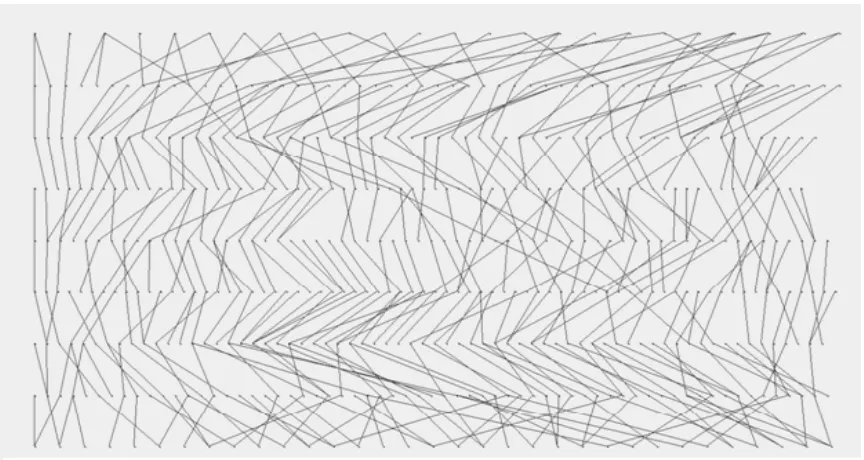
Figures 5.3 and 5.4 show 500 nodes, 9 layers and an aspect ratio of 32 trees after MCN and mod-bary has been applied to it.

Figure 5.3 MCN applied to a tree

(53)

Figure 5.4 Modified barycenter applied to a tree

5.3.5 Performance of MCN with iterations

Table 5.7 and Figures (5.5 through 5.8) show how MCN behaves with respect to number of iterations. MCN takes time to converge to an optimum solution as it acts on only one node in one iteration.

Table 5.7 MCN with iterations

Series % of Initial Crossings after Iteration#

8 16 32 64 128 256 512 1024 2048

Instance1 91.4 86.2 73.9 61.7 48 32.1 21.6 17.2 15.5

Instance 2 90.7 85 75.5 66 53.4 36.8 23.4 17.3 14.2

Instance 3 91.7 87.1 78.8 66.2 49.5 31.3 20.8 16 13.8

Instance 4 92 86.8 78.4 68.7 52.4 35 23.6 16 13.5

Instance 5 92.7 87.2 80 71 52.4 33.6 22.9 17.7 16

Instance 6 93.6 87.4 81.6 68.7 50.9 35.3 23.4 16 14.3

A 500 node, 9 layer, aspect ratio 32 tree after modified barycenter applied to it. Initial number of crossings = 7692. Number of crossings now = 844

(54)

Figures 5.5 to 5.8 show various stages of tree (Instance 1 of table 5.7) when MCN is applied to it.

Figure 5.5 8 iterations of MCN applied to a tree

A tree of 500 nodes, 9 layers and aspect ratio 32 after 8 iterations of MCN applied to it. Initial number of crossings = 7692. Number of crossings now = 7033

(55)

A tree of 500 nodes, 9 layers and aspect ratio 32 after 256 iterations of MCN applied to it. Number of crossings after 32 iterations = 5688. Number of crossings now = 2467

(56)

5.3.6 Effect of number of layers on minimum crossings iteration for MCN

Table 5.8 demonstrates how the iterations required to reach minimum crossings, given all other parameters are fixed, decreases with increase in the number of layers for a variety of aspect ratios. This is because, given the same number of nodes, the graph is more spread out and sparse in case of more number of layers.

Table 5.8 Minimum crossings iteration with layers for MCN

No. of

nodes/Aspect Ratio

Min. crossings iterations for 9

layers

Min. crossings iterations for 22

layers

500/1 3189 2231.6 500/32 3347.6 2262.1 500/128 3308.6 2441.1 500/512 3911.2 3757.5

5.3.7 Effect of depth first search (dfs) implementation for initial ordering on all heuristics

The next step in experiments is to study any effect of initial ordering of nodes by the conventional methods (like dfs). The initial ordering in trees by depth first search (dfs) leads to very good results. There is also a change in performance of the heuristics on a dfs sorted tree. MCN is a clear winner here and thus the combination of dfs and MCN is studied for later experiments.

(57)

Figure 5.9 Difference in crossings minimization of the heuristics due to dfs

Figure 5.9 shows clearly that there is a great increase in the performance of the heuristics once dfs is used for initial ordering. The change is smallest for modified barycenter. Simpler versions of traditional heuristics like simple barycenter and simple median are not able to improve upon the initial ordering produced by dfs. The winner here is MCN as when combined with dfs, it is able to produce crossings lesser than modified barycenter and is thus the best heuristic in case of trees. Table 5.9 shows the actual number of reduction in crossings when dfs is applied.

Table 5.9 Affect of dfs

Heuristic Initial Crossings

Crossings after dfs

Heuristic Crossings when no dfs dfs

Bary 7595.5 1246.3 6465.8 1246.3

Median 7595. 5 1246.3 6556.6 1246.3

mod- WEL 7595. 5 1246.3 3144.3 1246.3

MCN 7595.5 1246.3 1054.2 370.3

mod-bary 7595. 5 1246.3 926.1 728.9

mod-median 7595. 5 1246.3 1752.8 745.1

(58)

5.3.8 Performance of MCN + dfs with iterations

The iterations versus crossings table (Table 5.10) clarifies that the first 500 iterations (equal to the number of nodes in the graph) produces the maximum reduction in crossings. This happens because all the nodes are covered in first 500 iterations and they are positioned in such a way that they reach close to or at their position of minimum crossings contribution. Within the first iteration, once initial few nodes which contributes maximum to crossings are placed in a minimum crossings position, the rate of reduction in crossings decreases. This is due to the fact that the initial few maximum crossings nodes are the major contributor in the crossings of other nodes too. So once these are sorted, the remaining nodes only do a local adjustment within themselves.

That is why at any stage of iteration, the nodes are not likely to move in a way that there is an increase in total number of crossings in the graph. Thus the local optimum for any smaller instance of problem (which in this case is a node) at any stage also helps in optimizing the global solution (i.e., the crossings in the entire graph.) This is also depicted through figures 5.10 to 5.14.

Table 5.10 Graphs with dfs + MCN iterations

Series

% of Initial Crossings after Iteration# 0

(After dfs)

8 16 32 64 128 256 512 1024 2048

Instance1 19.6 17.6 16.9 14.5 10.6 8.3 7.6 6.8 6.5 6.2

Instance 2 19.4 17.3 16.2 13.0 7.0 5.1 4.8 4.3 4.3 4.3

Instance 3 15.7 15.5 13.2 11.5 8.7 6.8 6.6 5.6 5.5 5.5

Instance 4 16.7 15.7 12.8 10.0 6.5 5.5 5.2 4.2 4.2 4.2

Instance 5 13.9 10.7 9.4 9.1 7.1 6.6 6.4 6.2 6.1 6.1

Instance 6 14.4 12.8 9.7 6.4 3.5 3.0 2.9 2.8 2.8 2.8

Table 5.10 shows that the decrease in crossings is not uniform with iterations, and at initial stage of iterations there is a good decrease in crossings due to the adjustment of nodes contributing most in crossings.

(59)

Figures 5.10 to 5.14 show various stages of tree (Instance 1 of table 5.10) when initial ordering by dfs and MCN is applied to it.

Figure 5.10 Dfs applied to a tree

(60)

Figure 5.11 Dfs and 8 iterations of MCN applied to a tree

A tree of 500 nodes, 9 layers and aspect ratio 32 after dfs and 8 iterations of MCN applied to it. Number of crossings after dfs = 1508. Number of crossings now = 1352

(61)

A tree of 500 nodes, 9 layers and aspect ratio 32 after dfs and 256 iterations of MCN applied to it. Number of crossings after 32 iterations = 1115. Number of crossings now =

(62)

5.3.9 MCN vs. mod-bary treated graph

Modified barycenter affects the whole graph in its iteration, i.e., it sorts all the layers

in one iteration, and thus comes up with fewer crossings soon when compared to MCN. For a MCN treated graph, there are typically more edges with no crossings or just one crossing but some edges that are long and cross a lot of edges.

After few iterations of graph, crossings are more uniformly distributed over a mod-bary operated graph. Over a MCN operated graph, crossings are more non-uniformly distributed. If there are too many crossings at one place, mod-bary performs well than MCN. One reason can be because in MCN, only the node in consideration is moved while in mod-bary all the nodes of graph are moved. Thus, a more uniform picture of the graph comes for a mod-bary operated graph.

5.3.10 Performance of MCN with larger graphs

The number of iterations required to reach minimum crossings increases with the number of nodes in the graph.

(63)

This is because of two factors – the total iteration of graph (which is when all nodes of the graph are covered at least once) becomes bigger with increase in nodes, and also because with larger number of nodes there is more probability of some local optimization happening in later iterations.

In Figure 5.15, the X axis represents the number of iterations as percentage of nodes in graphs. Thus for a graph of 500 nodes, .2 on X-axis represents .2 x 500 = 100 iterations. For a graph of 1000 nodes, it represents .2 x 1000 = 200 nodes and 400 iterations for a graph of 2000 nodes. The figure clearly depicts how a larger number of iterations are significant in reduction of crossings with increase in number of nodes in the graph. For a n-node graph, the rate of reduction in crossings is highest and significant for the first iteration covering all the nodes of the graph, i.e., for the first n iterations.

Table 5.11 MCN performance with increase in nodes

No. of Nodes (n) Iterations/n 0.0(dfs only)

0.1 0.2 0.3 0.4 0.5 0.6 0.7 0.8 .9 1.0

500 16.4 8.6 6.2 5.9 5.7 5.6 5.6 5.3 5.1 5.0 5.0

1000 16.0 11.6 8.8 7.3 6.8 6.6 6.5 6.4 6.4 6.3 6.2

2000 15.7 13.3 11.5 10.1 8.9 8.1 7.5 7.2 7.1 7.0 6.9

Table 5.11 shows the data for crossings as percentage of intial crossings for various columns. Each column considers iterations which are contingent upon number of nodes in the graph as in figure 5.15. Thus for the first row, the number of iterations are .1x500, .2x500 and so on. Similarly, for second row it is .1x1000, .2x1000 and so on. The data in Table 5.11 re iterates the fact that for larger no. of nodes in the trees, more number of iterations are involved in reducing the crossings in the graph. Thus, if it takes 500 iterations for 500 node graph, it takes 1000 and 2000 iterations respectively for a 1000 and 2000 node graph to reach the same percentage of initial crossings.

(64)

5.3.11 Consistency of Heuristics

The two heuristics which performs best in case of trees, i.e., MCN and mod-bary are also checked for consistency. This is done by running the heuristics on an iso-class of 32 graphs and measuring their standard deviation and mean. A more consistent heuristic is expected to have a small standard deviation across an iso class.

Table 5.12 shows how the two heuristics behave over an entire range of trees. It is clear from Table 5.12 that modified baryenter is more consistent of the two heuristics. The percentage ratio of standard deviation to mean of minimum crossings lies between 5 to 12% for both the heuristics over the entire set of trees. Thus, the performance of both the heuristics in terms of consistency is good.

Table 5.12 Heuristics performance with isomorphism class

Nodes/ Layers/ Aspect Ratio MCN Mod-bary Min Mean Max Standard

Deviation

Min Mean Max Standard Deviation

500/9/1 804 1071.3 1320 106.1 742 870.4 970 54.5

500/9/2 900 1051.5 1368 102.1 850 956.2 1111 64.0

500/9/4 852 1027.8 1178 89.5 881 984.3 1106 50.7

500/9/8 907 1068.1 1242 104.2 783 920.2 1055 69.2

500/9/16 841 1116.4 1116.4 124.4 835 956.1 956.1 60.8

500/22/1 321 392.9 526 44.5 317 394.2 469 34.2

500/22/2 267 373.9 454 45.8 406 407 479 30.9

500/22/4 287 357.6 416 33.5 319 385.7 458 31.6

500/22/8 299 389.5 389.5 36.9 335 388.9 388.9 34.4 500/22/16 298 373.2 373.2 41.8 365 412.3 412.3 28.4

(65)

5.4 Results of experiments performed over dags

Experiments performed on the equal and unequal layer dags shows that there are no differences in the trend followed by heuristics in both the cases. Thus, only the results of experiments performed on equal layer dags are reported in this thesis.

5.4.1 Bary vs. Mod-bary

Experiments conducted on dags of equal layers shows that modified barycenter performs consistently better than simple barycenter over a wide range of dags as shown in Table 5.13. Various parameters of the input dags were changed including the number of nodes and edge density.

Table 5.13 Bary vs. Mod-bary on dags

Nodes/Layers /Edge Density Initial Crossings Bary mod-bary Min. Crossings % Crossings Min. Crossings % Crossings

500/9/1.5 17360.2 14640.6 84.3 5039.0 29.0

500/9/3 71666.2 64255.6 89.7 35829.6 50.0

500/9/9 652229 612370 93.9 471157.2 72.2

500/22/1.5 6469.3 5611.3 86.7 1905.6 29.5 500/22/3 25017.3 23723.8 94.8 12607.5 50.4 500/22/9 218398.2 213514 97.8 166949 76.4

5.4.2 Mod-bary vs. Mod-median

In the case of modified median and modified barycenter heuristic, modified barycenter performs better than modified median over the entire set of experiments conducted. Table 5.14 corroborates this.

(66)

Table 5.14 Mod-bary vs. Mod-median on a daag Nodes/Layers/ Edge Density Initial Crossings mod-bary mod-median Min. Crossings % Crossings Min. Crossings % Crossings

500/9/1.5 17360.2 5039.0 29.0 7058.4 40.7

500/9/3 71666.2 35829.6 50.0 41406.6 57.8

500/9/9 652229 471157.2 72.2 498635.8 76.4

500/22/1.5 6469.3 1905.6 29.5 2567.5 39.7

500/22/3 25017.3 12607.5 50.4 14557.2 58.2

500/22/9 218398.2 166949 76.4 175220.8 80.2

5.4.3 Modified Weighted Edge Length vs. Traditional Heuristics

Table 5.15 shows clearly that though modified WEL performs better consistently when compared to the simple version of traditional heuristics (both barycenter and median), it also performs consistently worse when compared with the modified barycenter. Thus, this heuristic is also not considered for future experiments.

Table 5.15 Mod-WEL vs. traditional heuristics on dags

Nodes/Layers /Edge Density

(bary)

(median)

% of Initial Crossings (mod-WEL)

% of Initial Crossings (mod-bary)

500/9/1.5 84.3 89.3 69.2 29.0

500/9/3 89.7 91.8 78.6 50.0

500/9/9 93.9 94.9 87.3 72.2

500/22/1.5 86.7 92.7 61.3 29.5

500/22/3 94.8 93.8 75.1 50.4

500/22/9 97.8 95.1 89.8 76.4

Minimum crossings and percentage of initial crossings after mod-bary and mod-median heuristics have been applied on a random class of 32 graphs of equal layer dag