ABSTRACT
MCDOWELL, EMILY BRIANNE. Adult Sex and Heath Estimation in a North Carolina Algonkian Population: The Piggot Ossuary (31CR14). (Under the direction of Dr. Ann Ross).
Estimating health in a skeletal sample is important for understanding various aspects of archaeological populations. From health, bioarchaeologists can make inferences about environmental stresses, and societal structure. The majority of methodologies that examine health are performed on individuals by looking at the affected elements; this makes
estimating health in ossuary settings difficult, as elements cannot be associated with a single individual. Furthermore estimating health is problematic without the consideration of biological sex. Examining differences in health between sexes can allude to sexual division of labor, while looking at overlap the sizes of males and females gives insight to the degree of population health. In addition, the estimation of sex is an essential first step in the reconstruction of past life ways as all other parameters such as stature, age-at-death are sex specific.
Ossuaries comprisethe majority of burials on the east coast during the Late Woodland period, considering the methodologies to sex elements and estimate health in ossuary scenarios is lacking, this portion of the archaeological record is largely unstudied.. Furthermore, coastal erosion and economic development have made many sites
unobservable, which has resulted in a paucity of information for coastal sites. This study aims to estimate sex and health in the Piggot ossuary (31CR14) a prehistoric coastal North Carolina Native American Algonkian speaking population.
Adult Sex and Health estimation in a North Carolina Algonkian Population: The Piggot Ossuary (31CR14)
by
Emily McDowell
A thesis submitted to the Graduate Faculty of North Carolina State University
in partial fulfillment of the requirements for the degree of
Master of Arts
Anthropology
Raleigh, North Carolina 2014
APPROVED BY:
_______________________________ ______________________________
Dr. Ann Ross Dr. Troy Case
Committee Chair
________________________________
DEDICATION
To Sir Pounce-A-Lot Felix Wutherford of Caterington: Mouse Bounty Hunter, for always keeping me on my toes, for being my soul mate, entertainer, troublemaker, little spoon and constant companion.
And to Miss Phineas Beatrice Von Catthroppe Version 2.0: Kat-Bot, for being the best foot warmer a person could ask for, having intelligent conversations, and for basically writing my thesis for me (seriously, she wrote like… the whole thing).
BIOGRAPHY
ACKNOWLEDGMENTS
Dr. Ann Ross
For suggesting this thesis idea, editing, editing, stats, editing, for letting me stab that pig neck, and for being a pretty awesome mentor
Dr. Troy Case and Dr. John Millhauser
For editing some more, which ultimately made my thesis better Amanda Hale
TABLE OF CONTENTS
LIST OF TABLES ... vi
LIST OF FIGURES ... vii
INTRODUCTION ... 1
REVIEW OF THE LITERATURE ... 4
Population Stress ... 4
Health Indices ... 6
Paleodemographic Studies ... 9
Health in North Carolina Populations ... 11
Previous Studies of the Piggot Ossuary ... 12
The Osteological Paradox ... 13
BACKGROUND ... 16
Late Woodland Period Algonkians ... 16
Algonkian Ossuaries ... 18
MATERIALS AND METHODS ... 21
The Piggot Ossuary ... 21
Reference Population ... 24
Methodology ... 25
RESULTS ... 31
DISCUSSION ... 49
Accuracy of the Sectioning Point ... 49
Health and Sexual Dimorphism ... 50
Considerations ... 55
CONCLUSION ... 56
REFERENCES ... 58
APPENDICES ... 69
LIST OF TABLES
Table 1: Measurement abbreviations and definitions. ... 26
Table 2: Multivariate and univariate descriptive statistics for the Averbuch. ... 31
Table 3: Sectioning points and formulae created from Averbuch reference population to be used on the Piggot ossuary. ... 35
Table 4. Correct Classification Results for Averbuch Sample ... 35
Table 5: Multivariate and univariate descriptive statistics for Piggot. ... 39
Table 6: Mahalonobis squared distances between males and females for the Piggot ossuary 43 Table 7: 95% confidence intervals for Piggot. ... 43
Table 8: Index of Sexual Dimorphism for Piggot and associated t-test and Wilcoxon Mann-Whitney results. ... 47
Table 9 Index of Sexual Dimorphism for Averbuch and associated t-test results. ... 47
Table 10 Crural Index for Piggot ossuary ... 48
LIST OF FIGURES
Figure 1 Coastal North Carolina Language Groups ... 17
Figure 2 Location of Piggot Ossuary (Garrett 2012) ... 23
Figure 3: Piggot ossuary in situ semi-circle of skulls from group F highlighted (Truesdell 1995). ... 24
Figure 4 PCA showing homogeneity of the Averbuch sample with red representing females and blue representing males ... 27
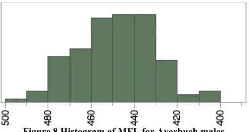
Figure 5 Histogram of MHH for Averbuch males ... 32
Figure 6 Histogram of MHL for Averbuch males ... 32
Figure 7 Histogram of MFH for Averbuch males ... 32
Figure 8 Histogram of MFL for Averbuch males ... 33
Figure 9 Histogram of MTL for Averbuch males ... 33
Figure 10 Histogram of MHH for Averbuch females ... 33
Figure 11 Histogram of MHL for Averbuch females ... 34
Figure 12 Histogram of MFH for Averbuch females ... 34
Figure 13 Histogram of MFL for Averbuch females ... 34
Figure 14 Histogram of MTL for Averbuch females ... 35
Figure 15: MTL plot for the Averbuch, Male=1 shown in blue Female=2/shown in red ... 36
Figure 16: MFH plot for the Averbuch, Male=1 shown in blue Female=2 shown in red ... 36
Figure 17: MHH biplot for the Averbuch, Male=1 shown in blue Female=2 shown in red ... 36
Figure 18: MFH+MFL biplot for the Averbuch, Male=1 shown in blue Female=2 shown in red ... 37
Figure 19: MHH+MHL biplot for the Averbuch, Male =1 shown in blue Female=2 shown in red ... 38
Figure 20 Histogram of MHH for Piggot males ... 40
Figure 21 Histogram of MHL for Piggot males ... 40
Figure 22 Histogram of MFL for Piggot males ... 40
Figure 24 Histogram of MTL for Piggot males ... 41
Figure 25 Histogram of MHH for Piggot females ... 41
Figure 26 Histogram of MHL for Piggot females ... 42
Figure 27 Histogram of MFH for Piggot females ... 42
Figure 28 Histogram of MFL for Piggot females ... 42
Figure 29 Histogram of MTL for Piggot females ... 43
Figure 30: 95% confidence interval for Piggot males and females for the MFL Male=1, Female=2 ... 44
Figure 31: 95% confidence interval for Piggot males and females for MHL Male=1, Female=2 ... 44
Figure 32: 95% confidence interval for Piggot males and females for MFH Male=1, Female=2. ... 44
Figure 33: 95% confidence interval for Piggot males and females for MHH Male=1, Female=2 ... 45
Figure 34: 95% confidence interval for Piggot males and females for MTL Male=1, Female=2 ... 45
Figure 35: 95% confidence interval for Piggot males and females for MHL and MHH Male=1, Female=2. ... 45
INTRODUCTION
The estimation of health is imperative for establishing important demographic
information about archaeological populations, such as social stratification and environmental stresses. But the methods used to develop health indices have been developed where
cemeteries or individual burials are common. Where commingled remains are more common, such as among cultures that buried their dead in ossuaries, health indices are rarely used. Furthermore, health is difficult to evaluate without the estimation of biological sex. Sex is most accurately estimated using the os coxa or the skull. However, in a commingled burial, skeletal elements cannot be associated with a single individual. Therefore, bones must be sexed by skeletal element instead of by individual.
Considering that ossuaries comprisethe majority of burials on the east coast during the Late Woodland period, this leaves a large piece of the archaeological record unstudied. Curry (1999) discusses the paucity of health studies on Maryland ossuaries: “in effect, what we have in the skeletal remains from Maryland Ossuaries is a vast pool of nutritional and
pathological data that has gone untapped, or at least has been tapped unevenly.”
This study aims to estimate the sex and examine the health of the Piggot ossuary (31CR14), a prehistoric coastal North Carolina Native American Algonkian speaking
Using the Tennessee Averbuch as a reference population, a sectioning point between males and females was calculated using a linear discriminant function (DFA) of the femora, tibiae, and humerii separately. The sectioning point was applied by element to the Piggot ossuary by utilizing equations also created from the DFA on the Averbuch. Any value that fell above the sectioning point was classified as male, while any value that fell below was classified as female.
After establishing sex, distances between measurements were analyzed to assess differences between male and female individuals. Based on the hypothesis that females are better able to canalize, or buffer, stress than males, it can be extrapolated that there would be a lesser degree of variation between males and females in an unhealthy population. It can also be assumed that out of the humerii, tibiae, and femora, the lower limbs are more
susceptible to stress. Moreover, the distal segments are more affected by stress, meaning that the tibia should be the most diagnostic determinant of health in the population (Fleagle et al. 1975) and this fact has been used to identify nutritional stressors in contemporary juveniles (Ross 2011, Ross and Juarez 2013). Biological relatedness was examined by calculating a Mahalonobis squared distance (D2), which compares the distance between the sexes in relation to a group mean, and by observing the degree of overlap between the sexes in each element’s 95% confidence interval.
correlates sexual dimorphism with population stress. Gray and Wolf (1980) note that as stress levels increase, sexual dimorphism within the population decreases. A t-test was performed on the means in both populations in conjunction with the ISD to account for variability in the population (Lockwood 1999). Because a t-test assumes a normal distribution of the data, a Wilcoxon Mann-Whitney test was also calculated for Piggot as the population proved to have skewed distributions of males and females, likely due to small sample sizes. The Piggot ossuary ISD was compared to that of the reference population (e.g. Averbuch) in order to assess the degree of health in the ossuary.
A crural index was also calculated to examine the size ratio between the femur and the tibia. Considering that individuals are commingled, the crural index was assessed using the group means of the tibiae and femora for both males and females for the Averbuch and Piggot samples. The closer the index value is to 100, the more similar the femora and tibiae were in size. Comparisons were made between males and females of both populations.
REVIEW OF THE LITERATURE
Population Stress
There are several traits exhibited by the skeleton that reflect population stress and therefore health. Humphrey and King (2000) note that long-term stress and chronic illness are more likely to manifest themselves in the skeleton through the appearance of Harris lines or lines of arrested growth, asymmetry, variation in limb proportions, and cranial base height. In their examination of childhood stress, they suggested that individuals with higher levels of stress early in life have a higher morbidity and mortality rate as well as a higher instance of disease than individuals with lower levels of early childhood stress. Sutphin and colleagues (in press) also found cranial length to be significantly affected in the Eastern and Western Cherokee bands due to environmental stress related in part to the forced migration west. For example, McDade (2003) has shown that even in utero a child’s health can be impacted due to nutritional deprivation of the mother. In the postnatal period, the amount of time a mother spends breastfeeding a child and the nutrition she is able to provide both impact overall health. McDade (2003) suggested that nutritional deprivation has a negative effect on a child’s immune system, which in turn negatively impacts their ability to fight off infectious diseases. The resources required to fight off infections early in life take away from the energy required for proper growth. Therefore, children with a lower immunity are at a higher risk of infection and are more likely to have periods of stunted growth.
example, Jantz and Meadows Jantz’s (1999) study on secular change in long bone length showed how change in males is more pronounced than in females. Stini (1982, 1985) contributes women’s ability to canalize stress more efficiently to them being more
biologically stable because of their capacity to bear children. He states that overall, men are more affected by environmental stress than women. Generally, there is a trend of reduced variation between men and women in more marginalized or stressed societies that is believed to be due to women’s ability to better buffer environmental stresses (Greulich 1971, Gruelich et al. 1953, Stini 1969, 1972, 1982, 1985, Jantz and Meadows Jantz 1999, Tanner 1962, Tobias 1972). Ross et al. (2003) further enforced this idea when testing for biomechanical versus environmental stresses in the forearm by looking at size and shape in an archaic sample. They observed that variation in the female forearm was solely attributed to shape and therefore biomechanical processes. However, they also note that variation in the male forearm is attributed to shape and size, indicating that both the environment and
biomechanical processes contribute to change. This suggests that females are better able to canalize stress than males, since the males are more impacted by environmental factors in this situation.
(1977) in their examination of the Kayapo from Brazil. They found that a decrease in sexual dimorphism in the arm did not relate to nutritional stress, but to females partaking in
strenuous physical labor normally associated with males.
Further studies suggested that, within the body, the distal limbs are more prone to variation caused by stress than proximal limbs and that lower limb change is more pronounced than upper limb change (Holliday and Ruff 2001, Jantz and Meadows Jantz 1999, Bogin et al 2002). Growth retardation is more likely to happen in the tibiae first, then in the ulnae, and radii than in the proximal elements such as the femur and humerus
indicating that proximal elements would show greater variation in length, which would be most notable in the tibia (Flegel et al. 1975, Holliday and Ruff 2001, Jantz and Meadows Jantz 1999).
Health Indices
Numerous studies have been performed on the health of both modern and
the study of health into four stages: the focus on quaternary fauna from 1774-1870; the focus on human trauma and syphilis from 1870-1900; the focus on infection and medical
interventions from 1900-1930; and the focus on disease in an ecological context from 1930 onward. Goodman and Martin (2002) focused on the changes in the history of health since Ubelaker’s 1982 publication. They stated that modern health has a technological focus that brings on a plethora of new research questions. The utilization of new scientific methods such as stable isotopes and DNA, as well as improvements to the methodologies behind health indices and paleodemographic studies, and a better understanding behind osteological morphology have greatly increased the knowledge of health in past populations.
One of the most commonly used measures of past health is a health index. Health indices rank individuals according to a variety of skeletal indicators in order to create a score that makes populations temporally and geographically comparable. In most studies, health indices are calculated on an individual basis because the estimation of sex and age-at-death are necessary for most index methodologies. One of the more popular health index
methodologies was developed by Steckel et al. (2002). This method requires each skeleton in the index to be sexed, and aged, given an estimated stature, scored systemically for
2002). However, the requirement to utilize as much of an individual as possible makes the method difficult if not impossible to apply in commingled scenarios.
Other assessments of health are based on fewer attributes than those used by or variants of Steckel et al. (2002) and encompass either the individual or the overall population. Neves and Costa (1998) developed a health index based on height, using the femur as a proxy for stature. They assumed that unhealthy populations exhibited less
variation in stature because women are better able to canalize stress than men. By comparing how similar males and females were in size, they determined the health of prehistoric
Atacama Desert populations.
In another approach, Lambert (1993) used the maximum dimension of periosteal lesions and stature as an indicator of temporal health in the Santa Barbara Channel Islands. She calculated an index of severity using the maximum lengths of lesions divided by the maximum lengths of bones. Stature differences were established by calculating the distance of each femur from the mean and tested with a t-test to assess if significant differences existed between populations from varying time periods. Lambert discovered a general decline in health over time in the islands.
hypothesis that nutritional stresses occurred in the Town Creek population despite periodic episodes of drought (Cunningham 2010). Pretty and Kricun (1989) examined the health of a prehistoric aboriginal population from Australia. They observed stature differences, the
frequency of growth recovery lines (Harris lines), dental health, pathologies, trauma and
general skeletal anomalies. They determined that the Roonka aborigines were healthier than
previously thought and that their small population probably represented a wider regional area
(Pretty and Kricun 1989). Larsen et al. (2007) examined femur length as a proxy for stature
at the Windover Bog site in Florida. They found minimal fluctuation in femur length over
time and concluded that the population likely faced marginal amounts of stress (Larsen et al.
2007).
The number of health indices performed on various sites from around the world is
expansive because health has become a commonly studied aspect of archaeological
populations, which has also been explored in forensic settings (Danforth et al 1994, Steckel
2003, Iezzi 2009, Pitts and Griffin 2012, Danforth et al 2007, Roberts and Cox 2007, Blau
2007, Passalacqua et al. 2011, Maxwell and Ross 2011). However, health is population
specific and requires a range of methods to encompass the variety of conditions remains can
be found in.
Paleodemographic Studies
Similar to health indices, paleodemographic studies measure the health of a
focus on mortality, and require age-at-death of individuals be known. Despite its frequent use, paleodemography is highly criticized (Buikstra and Koningsberg 1985, Boquet-Appel and Masset 1981, Ubelaker 1974). Ubelaker (1974) discussed the three major flaws of paleodemography: it assumes that the sample is complete and representative of a population; it assumes age-at-death estimations are accurate; and it assumes that the population had a constant mortality rate in comparison to the size of the population. Techniques used to estimate age-at death, in particular, become less reliable as individuals get older. This skews the mortality curves created for populations and gives an unrealistic picture of population health.
Another critique is that many paleodemographers are using incorrect statistical analyses to predict health (Buikstra and Koningsberg 1985, Chamberlain 2003). Despite efforts to improve statistical techniques (see Konigsberg and Frankenberg 2002), there has been little improvement in the accuracy of age-at-death estimation for older individuals. For instance, new developments into age-at-death assessment from tooth root translucency height have proven to be unreliable past the age of 40 (Lamendin 1992, Prince and Ubelaker 2002).
Over the last two decades further improvements have been suggested for
paleodemographic studies (Chaimberlain 2003, Hoppa and Vaupel 2002), and progress has been made in examining solutions to the inherent shortcomings seen in the field
(Chamberlain 2006, Konigsberg and Frankenberg 2002). Despite the flaws in
Health in North Carolina Populations
Previous studies on the health of North Carolina populations are focused mainly along the coast. Hutchinson (2002) compared the inner and outer coastal populations to explore health via diet using stable isotopes. He concluded that late woodland inner coastal populations had an agricultural diet heavy on maize, while the outer coastal populations relied mainly on foraging. Hutchinson (2002) also examined the population for dental caries, cranial and postcranial lesions, cribra orbitalia, porotic hyperostosis, and osteoarthritis. Because many argue that there is a decline in health after the introduction of agriculture (Stuart-Macadam 1987, Cohen and Kramer 2007), it would be expected that inner coastal populations who relied more heavily on a maize diet were less healthy in comparison to outer coastal populations. However, Hutchinson (2002) found that the frequency of cribra orbitalia and porotic hyperostosis was 44% in outer coastal populations, while only 20% in inner coastal populations. In a reanalysis of this study, Hutchinson (2007) discussed the possibility of a higher rate of intestinal parasites in outer coastal populations due to their marine-based diets.
Vasalech (2011) noted that porosity in the orbital plate seen in adults is more consistent with the type seen from vitamin deficiencies and is in agreement with Hutchinson’s (2007) hypothesis that the high presence of cribra orbitalia in outer coastal populations is due to intestinal parasites. Both Hutchinson’s (2002, 2007) and Vasalech’s (2011) findings suggest that populations present along the North Carolina coast were unhealthy.
Previous Studies of the Piggot Ossuary
As noted earlier Hutchinson’s (2002, 2007) stable isotope study utilized the Piggot ossuary as a Late Woodland outer coastal population in order to compare the diets of inner and outer coastal populations.
Garrett (2012) focused on making the collection synonymous with North Carolina and Federal curation standards. After processing and cataloguing, she performed an
osteological examination, which is a demographic overview of the population. She estimated the minimum and most likely number of individuals and created a mortality curve based on age-at-death estimates. She also discussed the implications of the presence of cribra orbitalia, porotic hyperostosis, and osteomyelitis in the population and concluded that the population had a large amount of disease present.
clear age markers. However, a paleodemographic study such as Truesdell’s (1995) could only be performed on a by-element basis and not by individual. Furthermore, because age-at-death becomes more difficult to estimate as individuals get older it is likely that adult health was not accurately assessed in this study. Notably, Truesdell discovered evidence of treponemal infection and argued that the signs of treponematosis were specifically congenital syphilis, which is consistent with studies done on several other North Carolina Coastal ossuaries (Bogan 1989).
The Osteological Paradox
The osteological paradox is the concept that those individuals that appear to display the most amount of skeletal stress are actually healthier than those individuals that show little to no skeletal markers of stress (Wood et al. 1992). While the osteological paradox is
becoming an inherent part of bioarchaeological studies since its introduction in 1992, its relationship with population health makes it relevant to the discussion of the literature. The osteological paradox is confounded by two important problems when studying human skeletons: selective mortality and hidden heterogeneity of risks. These two problems are inextricably linked when investigating past populations.
In Wood and colleagues (1992) foundational explanation of the osteological paradox, they argue that selective mortality refers to the inherent bias in the samples used under study as they are not necessarily representative of the living population as they did not survive. As a result, it is impossible to study all individuals in the population that were affected by
same age, but continued living, would not present themselves in the same demographic age groups as those who died. Furthermore, the examination of older individuals in a population does not necessarily indicate the types of health risks that those individuals may have
experienced throughout their lives. It must also be remembered that in many instances, lesions represent a chronic disease that occurred over a period of time, while acute diseases, which cause death over a shorter period of time, do not usually present themselves in the osteological record. This can cause an underestimation of health risks present in the population. This, coupled with the fact that it is impossible to have a representation of the “entire population at risk” (Wood et al. 1992), makes it difficult to extrapolate what was happening in the past.
Wood and colleagues (1992) further explained how hidden heterogeneity of risks refers to each individual’s ability to handle environmental and nutritional stresses. The ability to buffer stress differs among individuals and between groups, because it has genetic influences. Each person can buffer certain amount of environmental or nutritional stress before it becomes phenotypically apparent as a health risk. Those with a better ability to buffer stress are more likely to live through stressful situations and continue on into older generations. This allows selective mortality to present itself through hidden heterogeneity of risks and makes it impossible to determine “age-specific” and “aggregate-level” mortality rates in groups of individuals (Wood et al. 1992).
of both, the simplest of which is to be aware of its existence and to take into account its innate presence in making interpretations from archaeological samples. It must be remembered that bioarchaeologists can really only examine a moment in the life of an individual, by observing the way his or her body was preserved at the time of death.
BACKGROUND
Late Woodland Period Algonkians
In North Carolina, the Late Woodland period extends from A.D. 800 to A.D. 1650
(with A.D. 1650 representing European Contact). Several populations make up the Carolina
Late Woodland period including those found in the Piedmont, the Western Mountain Region
and the Coastal Plain (Phelps 1983). Of these populations, those found along the Coastal
Plains are the least examined because of looting and because of environmental and
developmental changes that have damaged many sites (Killgrove 2009). Late Woodland
coastal populations are characterized by three major linguistic groups: the Algonkian,
Iroquoian and Siouan (Killgrove 2009)(Figure 1). Of the three groups, the Iroquoian resided
along the inner Carolina coast, while the Siouan occupied the southern portion of the coast.
The Algonkian language group represents the outer Tidewater region of the coast, which
extends from the major sounds to the Barrier Islands (Killgrove 2009). The Carolina
Algonkians were the southernmost manifestation of a language group that extended up the
coast into Canada (Phelps 1983), and that included the Chowanoke, Weapemeac, Poteskeet,
Moratoc, Roanoke, Secotan, Pomuik, Neusiok, and Croaton tribes (Goddard 1978). The
majority of the information regarding Algonkian societies comes from post-contact
observations, such as Thomas White’s Roanoke voyages (Ward and Davis 1999). However,
assumptions can be made about the pre-contact era based on native histories recorded during
Figure 1 Coastal North Carolina Language Groups
According to Killgrove (2009), the Late Woodland was a period of change in which
many groups in North Carolina were becoming more sedentary and politically complex.
Over the span of several hundred years, groups became focused around a large population
center and political units developed to the size and complexity that were ultimately
encountered by Europeans during contact.
The Piggot Ossuary falls under the Late Woodland outer coastal Colington phase,
which is characterized by its Colington pottery, Roanoke triangular type and Clarksville type
hunting, while the populations of the inner coast depended on the cultivation of maize
(Hutchinson 2002). Pottery was a distinguishing characteristic between time periods, and the
shell-tempered Colington period pottery easily differentiates it from other periods and phases
(Phelps 1983). Killgrove (2009) says of the Colington pottery, “ceramics are fabric
impressed, but also include simple stamped, plain, and incised surface treatments.” The
Colington pottery is the most distinguishing feature of the Colington phase, and is one of the
primary distinguishing characteristics between Colington and Cashie phase populations
(Killgrove 2009, Phelps 1983). The Colington phase is contemporaneous with the inner
coastal Cashie phase, which is represented by a different set of tools and ceramics and
smaller ossuaries (Phelps 1983).
Algonkian Ossuaries
Ossuaries are burials containing the commingled remains of multiple individuals of
various ages and sexes. Typically, ossuaries are the result of a secondary burial, meaning that
individual remains were kept elsewhere for a time before being interred as a group (Curry
1999). Although the remains vary in treatment, they were often defleshed, disarticulated,
cremated, or removed from a primary interment before secondary interment. Primary
interment is the placement of the body directly into the ground after death; this is uncommon
in ossuary burials. Curry (1999) also notes that ossuaries are typically used by a single group
of people and are usually representative of a “population” at least for a short period of time.
According to Curry (1999), ossuaries along the North American coast were a symbol
return to earlier ossuaries for interment. For example, the Nanticokes of Maryland carried
their ancestors from their primary burial site on the Eastern Maryland shore through
Bethlehem Pennsylvania to inter their ancestors in ossuaries from their former village (Curry
1999). Ward and Davis (1999) note that bodies were likely placed in charnel houses to
decompose before being moved to their respective ossuaries.
Ossuaries are common in the mid-Atlantic region and become a defining
characteristic of the Late Woodland period. Among North Carolina Native American
populations, ossuaries arose in the Late Woodland period, as a new burial pattern attributable
to groups becoming more focused around a population center (Killgrove 2009). Jirikowic
(1990) believes that ossuaries present in coastal Maryland populations are a reflection of the
political system of chiefdoms that developed right before contact. Despite their frequency,
these ossuaries are poorly understood, particularly in the coastal regions. Algonkian ossuaries
were typically situated along the edge of a village, which contained a myriad of burial
treatments including articulated, disarticulated, and cremated remains. Grave goods are rarely
found in Algonkian ossuaries, and those that are show no patterns that suggest social or
economic differences (Curry 1999, Hickerson 1960). It is likely that the lack of burial goods
in Algonkian ossuaries is a result of bodies being revered during primary deposition in
charnel houses and being deposited in the ossuaries later (Hickerson 1960).
According to Phelps (1983), the inner and outer Carolina coast differed in their
ossuaries. The inner coastal Cashie phase ossuaries were small, with anywhere from two to
five individuals, and were thought to be family-oriented. The Algonkians along the outer
argues that these larger ossuaries were communal burials of social groups larger than
MATERIALS AND METHODS
The Piggot Ossuary
The Piggot ossuary (31CR14) contains the remains of a Late Woodland Algonkian
coastal population (Phelps and Cande 1975). It was located in the town of Gloucester in Carteret County, North Carolina. It was discovered when members of the Piggot family noticed human remains coming out of a crumbling creek bank on their property (Figure 2). David Phelps and a crew from East Carolina University first excavated the site in 1975 and again in 1980. Phelps (1977) speculated that the remains were affiliated with the Neusiok tribe, one of the southernmost of the Algonkian-speaking tribes. Conventional radiocarbon dates estimated the site at 410+/- 50 BP, about 1450 AD with calibrated dates of 1420-1640 AD, which dates it as a Late Woodland/Historic contact site (Truesdell 1995). However, newer radiocarbon dates on the age of this site puts it well within the Late Woodland phase,
likely before contact (Ross, Personal Communication).
The ossuary pit was located in a shell-midden, which provided a good context for the preservation of bone (Hutchinson 2002). The pit measured 1.8 meters wide by 3.4 meters long with a depth of 30-50cm, and was excavated into six groups labeled A through F based on possible clusters of individuals (Phelps and Cande 1975) Garrett (2012 ) notes an
additional surface collection labeled “group beach.” Truesdell (1995), in personal
semi-circle (Figure 3). The ossuary remained relatively intact upon excavation and was located in a shell midden with both prehistoric and historic ceramic, shell, and glass artifacts as well as faunal remains (Garrett 2012).
The condition of the remains was relatively good due to environmental preservation from the shell midden. However, some of the remains are fragmentary. Truesdell (1995) utilized Medlock’s (1975) method of estimating the minimum number of individuals (MNI) and estimated 84 individuals based on number of femora present after pair matching. Using Koningsberg and Adams’ (2004) methodology, Garrett (2012), estimated the most likely number of individuals (MLNI) to be 121 based on the femora, tibiae, humerii, and os coxae after pair matching.
Figure 2 Location of Piggot Ossuary (Garrett 2012)
Figure 3: Piggot ossuary in situ semi-circle of skulls from group F highlighted (Truesdell 1995).
Reference Population
Thus, based on these factors the Averbuch was selected as the most appropriate and available reference population.
Hugh Berryman (1984) originally published raw data from the collection in a chapter of the second volume of Averbuch: A Late Mississippian Manifestation in the Nashville Basin. The Averbuch are a Middle Cumberland Mississippian population located in the Nashville Basin in Davidson County, Tennessee. The site was first excavated by William Bass and Walter Klippel in 1977 and 1978 (Klippel and Bass 1984). The site is dated
between A.D. 1275 and A.D. 1300, is comprised of three cemeteries and is characterized as a chiefdom society that relied on maize agriculture. Berryman (1984) aged, sexed and
recorded standard measurements for each individual. The cemeteries represent a total of 710 individuals. However, only 321 were used in this study that were taken from the published literature.
Methodology
Data were selected from the Averbuch Skeletal collections database, individuals under the age of 18 who could not be sexed, or skeletons that did not have at least one of the required measurements were not considered. The measurements utilized were the maximum length of the humerus (MHL), the maximum height of the humeral head (MHH), the
Descriptive statistics were examined for both the Averbuch collection and the Piggot ossuary to determine if the data was normally distributed and assess means and sample sizes. Histograms were generated to represent the distribution of the data.
Statistics
A principal components analysis (PCA) was performed on the Averbuch
measurements in order to determine if any patterns could be attributed to any variable other than sex and to clarify that the Averbuch was appropriate as a reference population. A PCA assumes no correlation in a sample and reduces the dimensionality of the variation present in the sample. A PCA was performed to examine the homogeneity of the Averbuch skeletal sample and results showed that no variation was present that was not attributed to sex (Figure 4).
Table 1: Measurement abbreviations and definitions.
Measurement Description
Max length of humerus (MLH)
Distance from the most superior point on the head of the humerus to the most inferior point on the trochlea.
Max height of humeral head (MHH)
Maximum diameter on the border of the articular surface of the humeral head.
Max length of femur (MFL)
Distance from the most superior point on the head of the femur to the most inferior point on the distal condyles.
Max height of femoral head (MFH)
The maximum diameter of the femoral head
Max length of tibia (MTL)
Distance from the superior articular surface of the lateral condyle to the tip of the medial malleolus.
Figure 4 PCA showing homogeneity of the Averbuch sample with red representing females and blue representing males
Before creating sectioning points, significant outliers for the Averbuch were
recognized in the JMP 11.0 program and were then removed from the database. A combined total of 6 humeral and femoral measurements were removed. In each instance removal of outliers resulted in greater accuracy for the sectioning point. Outliers were not removed for tibial length measurements for several reasons. For example, each time an outlier was removed, additional outliers would be observed. The removal of outliers also resulted in a decreased accuracy of the sectioning point.
A linear discriminant function analysis (DFA) was performed on MHH, MFH and MTL, on MHL and MHH together, and on MFH and MFL together. DFAs were separated by bone for the Averbuch because Piggot is an ossuary and each element cannot be
associated with an individual, therefore an overall examination of the variables was not applicable. Length measurements for the humerus and femur were not available for all Piggot elements because of fragmentation; therefore they were not utilized in a univariate
Eigenvalue 4.1114 0.4584 0.1911 0.1360 0.1030
20 40 60 80
-6 -4 -2 0 2 4 6
Component 2 (9.17 %)
-6 -4 -2 0 2 4 6
Component 1 (82.2 %)
-1.0 -0.5 0.0 0.5 1.0
Component 2 (9.17 %)
MHL MFL MFH MHH
MTL
-1.0 -0.5 0.0 0.5 1.0
analysis. A linear DFA predicts sex by the selected measurement or measurements and determines the accuracy of the prediction. After running a DFA on all aforementioned measurements and their combinations, it was found that univariate measurements were more accurate than combined variables for sex estimation (Table 3). As a result, formulae for sex estimation of the tibia, femur, and humerus were created from single measurements only. The formula for sex estimation was modeled after Asala et al.’s (2004) equation:
P= (Mx)+y
Where P=predicted sex, M= the measurement of the bone, x= the unstandardized scoring coefficient, and y= discriminant function constant.
A sectioning point was created by taking the mean of the group centroids. A sectioning point is the mid point of the DFA, if the result of the above equation is greater than the specified sectioning point, the individual is classified as male, if it is less than, the individual is classified as female. The formula for the sectioning point was modeled after Asala et al.’s (2004) equation:
S= (m+f)/2
Where S= the sectioning point, m= the male group centroid, and f= the female group centroid.
were utilized, and any result above the associated sectioning point was scored as male, while any result below was scored as female. Following sex estimation for the Piggot elements using the newly derived sectioning points from the reference sample, a discriminant function analysis was run in SAS in order to generate Mahalonobis squared distances (D2). This determines if the biological distance between the sexes is significant (α =0.05) when compared to each group’s multivariate mean (JMP 11.0). A significant difference would indicate sexual dimorphism in the population. Mahalonobis squared distances were examined for MTL, MHH, MHL, MFL and MHF individually and for MHH and MHL combined and MHF and MFL combined.
Distance in variation between the variables was also used to ensure a definitive amount of separation between sexes. The canonical variates confidence intervals were analyzed because they represent only the variation present between the sexes, as canonical variates are a result of the correlation between the D2 values. In examining the confidence interval of the canonical scores a large amount of overlap would indicate a lesser degree of sexual dimorphism.
An index of sexual dimorphism (ISD) was used to assess the level of sexual dimorphism and stress within both the Averbuch and Piggot populations (Humphries and Ross 2011, Lockwood 1999). An ISD determines differences in body size between the sexes and because as stress increases, dimorphism decreases, the ISD can be correlated with
ISD= {(male mean/female mean)-1] x100}
According to Lockwood (1999), because an ISD compares mean values but does not consider variability between the sexes, a student’s t-test should also be used to test for sexual
dimorphism. A t-test assumes that the population is normally distributed, the variances are equal and that the variables are independent and continuous. A two-sample student’s t-test, was run in JMP v. 11.0 on of the length of the humerii, tibiae and femora and on the femoral and humeral heads to test for a significant difference (α=.05) in the means in both the Averbuch and the Piggot populations. Because the Piggot ossuary was not normally distributed for males or females a non-parametric Wilcoxon Mann-Whitney test, was also performed.
Additionally, a crural index was calculated for Piggot and the Averbuch, using the means of the tibiae and femora of males and females, as individuals were not available for comparison in the Piggot. A crural index is a ratio of the length of the femur in relation to the tibia. This ratio indicates the degree of difference seen between the tibiae and femora, the closer the tibiae and femora are in length the closer the index value is to 100 (Davenport 1933). A stressed population, in which distal and lower limbs were more affected (i.e. the tibia), would theoretically report a lower index value. A comparison of this index between males and females is indicative of size differences between the two. The crural index is calculated as:
RESULTS
Histograms showing the distribution of the Averbuch can be found in Figures 5-14. Both the males and females in the Averbuch population exhibited normality. Means and sample sizes for the Averbuch group are presented in Table 2. Multivariate and univariate means are presented separately for males and females. Sex estimation equations derived from the Averbuch are presented in Table 3. Formulae with multiple variables are included
although they were not utilized in sex estimation for the Piggot ossuary. Correct
classification results are presented in Table 4. Overall, males were more often misclassified as females in the Averbuch, which must be considered, as it may affect correct classification of the Piggot ossuary. DFA biplots for the Averbuch skeletal data are presented in Figures 5-9, the biplots clearly show the separation between males and females.
Table 2: Multivariate and univariate descriptive statistics for the Averbuch.
Multivariate Group Means Univariate Group Means
Sex N MFL MFH Sex N MTL
M 79 450.70886 46.03797 M 96 373.77083
F 73 423.31507 40.89041 F 69 342.73913
All 152 437.55263 43.56579 All 165 360.79394
MHL MHH MFH
M 87 323.77011 44.6092 M 106 46.084906
F 81 299.09877 38.67901 F 95 40.8
All 168 311.875 41.75 All 201 43.587065
MHH
M 95 44.757895
F 89 38.707865
Figure 5 Histogram of MHH for Averbuch males
Figure 6 Histogram of MHL for Averbuch males
Figure 8 Histogram of MFL for Averbuch males
Figure 9 Histogram of MTL for Averbuch males
Figure 11 Histogram of MHL for Averbuch females
Figure 12 Histogram of MFH for Averbuch females
Figure 14 Histogram of MTL for Averbuch females
Table 3: Sectioning points and formulae created from Averbuch reference population to be used on the Piggot ossuary
Single Male
centroid Female Centroid Sectioning Point= (m+f)/2
Accuracy Unstandardized Coefficient
Constant Formula
MHH 1.346 -1.437 -0.0455 91.3% 0.4595 -18.383
P=(M*0.4595)-18.383
MFH 1.323 -1.4763 -0.07665 91.5% 0.5281 -22.548
P=(M*0.5281)-22.548
MTL 0.7116 -0.9901 -0.13925 84.9% 0.0543 -19.594 P=(M*. 0543)-19.594
Multiple
MHH MHL
1.31 -1.435 -0.0625 91.0% 0.416
0.0089
-20.317 P=(M1*0.416)+(M2*
0.0089)-20.317
MFH MFL
1.256 -1.358 -0.051 90.1% 0.498
.00414
-22.028 P=(M1*0.498)+(M2*
0.00414)-22.028
Table 4. Correct Classification Results for Averbuch Sample
Sex M F
MTL M 78 18
F 7 62
MFH M 94 12
F 5 90
MHH M 84 11
F 5 84
MFL+MFH M 68 11
F 4 69
MHL+MHH M 75 12
Figure 15: MTL plot for the Averbuch, Male=1 shown in blue Female=2/shown in red
Figure 16: MFH plot for the Averbuch, Male=1 shown in blue Female=2 shown in red
Figure 19: MHH+MHL biplot for the Averbuch, Male =1 shown in blue Female=2 shown in red
Group means and sample sizes for Piggot can be found in Table 5, they are split between combined and single group means for all measurements. Histograms showing the distribution of Piggot can be found in Figures 20-29 males and females in the Piggot ossuary showed abnormal distributions likely due to small sample sizes. Out of the observed
Piggot can be found in Table 6. Similarly, 95% confidences intervals of the canonicals coincided with variables that demonstrated significant sexual dimorphism. MFH, MHH and MFH and MFL combined, and MHL and MHH combined, showed no overlap in confidence intervals, while MTL, MHL, and MFL had a high degree of overlap. Upper and lower boundaries of each 95% confidence interval can be found in Table 7, Figures 10-16
represents graphical depictions of each confidence interval with means. A complete list of measurements by bone, estimated sex, and calculated results of formulae applied to
sectioning points can be found in Appendix 1.
Table 5: Multivariate and univariate descriptive statistics for Piggot.
Multivariate Group Means Univariate Group Means
Sex N MFL MFH Sex N MTL
Sex N MHL
M 4 439 43.9675 M 4 370.75
M 4 299.25
F 8 427.625 41.13875 F 8 349.125
F 7 307.42857
All 12 431.41667 42.08167 All 12 356.33333
All 11 304.45455
MHL MHH MFH
MFL
M 4 299.25 41.68 M 7 43.518571
M 4 439
F 7 307.42857 38.86857 F 12 41.120833
F 8 427.625
All 11 304.45455 39.89091 All 19 42.004211
All 12 431.41667
MHH
M 6 43.1
F 7 38.868571
All 13 40.821538
Figure 20 Histogram of MHH for Piggot males
Figure 21 Histogram of MHL for Piggot males
Figure 23 Histogram of MFH for Piggot males
Figure 24 Histogram of MTL for Piggot males
Figure 26 Histogram of MHL for Piggot females
Figure 27 Histogram of MFH for Piggot females
Figure 29 Histogram of MTL for Piggot females
Table 6: Mahalonobis squared distances between males and females for the Piggot ossuary
Measurement D2 P-Value
MFL 0.6094
MFH 0.0077
MHL 0.86474
MHH 0.0002
MTL 0.3202
MFL/MFH 0.0287
MHL/MHH 0.0211
α =0.05
Table 7: 95% confidence intervals for Piggot.
MHL MHH
Lower 95% Upper 95%
MFL MFH
Lower 95%
Upper 95%
M 26.69 31.6 M 55.13 57.78
F 23.96 24.96 F 52.3 54.08
MTL MHL
M 43.59 42.65 M 30.41 31.18
F 48.26 43.84 F 32.35 33.3
MHH MFL
M 24.11 22.56 M 42.28 45.35
F 23.52 26.99 F 41.83 43.53
MFH
M 40.07 30.41
Figure 30: 95% confidence interval for Piggot males and females for the MFL Male=1, Female=2
Figure 31: 95% confidence interval for Piggot males and females for MHL Male=1, Female=2
Figure 33: 95% confidence interval for Piggot males and females for MHH Male=1, Female=2
Figure 34: 95% confidence interval for Piggot males and females for MTL Male=1, Female=2
Figure 36: 95% confidence interval for Piggot males and females for MFL and MFH Male=1, Female=2.
Table 8: Index of Sexual Dimorphism for Piggot and associated t-test and Wilcoxon Mann-Whitney results.
T-test Wilcoxon
M F ISD DF P-Value P-value
MTL 370.75 349.13 6.19 3.72 0.0145 0.0082
MHL 299.25 307.43 -2.66 9.00 0.9302 0.18
MFL 439.00 427.63 2.66 6.37 0.0527 0.1
MFH 43.52 41.12 5.83 15.72 <.0001 0.0005
MHH 43.10 38.87 10.89 6.20 0.0025 0.0034
Alpha=.05
Table 9 Index of Sexual Dimorphism for Averbuch and associated t-test results.
M F ISD DF P-Value
MTL 373.77 342.74 9.05 139.09 <.0001
MHL 322.36 298.94 7.83 192.66 <.0001
MFL 447.86 421.98 6.13 203.50 <.0001
MFH 46.08 40.8 12.94 198.96 <.0001
MHH 44.75 38.71 15.60 179.28 <.0001
Table 10 Crural Index for Piggot ossuary
M F
MTL 370.75 349.125
MFL 439 427.625
Crural Index 84.45 81.64
Table 11 Crural Index for Averbuch collection
M F
MTL 373.77 342.74
MFL 447.86 421.98
DISCUSSION
Accuracy of the Sectioning Point
First and foremost, it must be mentioned that the percentage of accurately sexed individuals reported for the Averbuch do not necessarily relate to the percent correctly classified in the Piggot sample. As previously mentioned, the sectioning point sexes individuals based on the resulting value of an associated equation being above or below the sectioning point. Accuracy is compromised because skeletal differences vary from
population to population, the dietary, spatial and temporal differences between the Averbuch cemeteries and the Piggot ossuary assumes some skeletal differences, particularly differences between the sexes. This results in a decreased accuracy of individuals correctly classified, because formulae created from the Averbuch site are being used on the Piggot population. As noted, the Averbuch equations have an increased propensity to incorrectly sex males as females (Table 4), which is reflected in the Piggot sample. As seen in Table 5, of the 13 total humerii, 6 were sexed as female (38%), of the 19 total femora, 12 were sexed as female (63%), and of the 12 total tibiae, 8 were sexed as female (67%). In both the femora and tibiae over half of the individuals were classified as female and it is likely that at least some of these individuals were males and misclassified as females.
attempt to sex skeleton from the Piggot site using Bass’s (2005) standard measurements for the femur, Garrett (2012) found that the majority of length measurements fell within the adolescent range indicating a “lack of adult elements” or a more gracile population.
Health and Sexual Dimorphism
Issues of sexual classification aside, the Piggot population exhibits several interesting results. Both the femoral and humeral head proved to be accurate estimators of sex; this is true for the Averbuch as well. This is expected because bones mature in circumference faster than they mature in length, thus features such as the femoral and humeral head reach their full growth potential earlier and are therefore less affected by environmental stresses. The humeral and the femoral head are commonly used in sex estimation and are preferred over the use of length measurements (Milner and Boldsen, 2011, Spradley and Jantz, 2011 , Ross and Manneshci 2011). As can be seen in Tables 6 and 8, the MFH and MHH of the Piggot population proved to be significant in, the D2 (MFH=0.0077 and MHH= 0.0002), and the t -test for the ISD (MFH=<0.0001, MFH=0.0025) and the Wilcoxon Whitney Mann test
Predictably, as was the case for the Averbuch, length measurements on their own were not accurate indicators of sex for Piggot (Tables 6 and 8). This is because as bone length is more affected by environmental stress, it takes longer to reach full growth potential. As previously noted, size differences such as length, are typically correlated with
environmental stress while shape differences, such as robusticity, coincide with biomechanical stress (Ross et al 2003). As a result, length measurements are a better
indicator of health and are often used as a proxy for stature in health estimation, particularly the femur as it is most highly correlated with stature (Steckel 2002, Lambert 1993, Larsen 2007). Shorter populations with less sexual dimorphism are often marginalized and under duress (Bogin et al. 2002). While the femur is the best proxy for stature, overall differences in bone length and proportion can parallel studies that focus on stature as an elements inability to reach its full growth potential would directly affect the height of an individual.
Additionally, the idea that women are better able to canalize stress than men implies that they are more likely to reach their full growth potential in stressed environments (Neves and Costa 2013, Jantz and Jantz 1999, Greulich 1971, Gruelich et al. 1953, Stini 1969, 1972, 1982, 1985, Jantz and Meadows Jantz 1999, Tanner 1962, Tobias 1972). This means that a stressed population would likely exhibit a lesser degree of dimorphism in terms of element size, something that becomes apparent in stature differences. Considering this study focused on size differences, results are likely indicative of environmental stresses and health.
treatment to males in childhood, which allowed them to more closely approximate their full growth potential. This differential access to resources reduced the variation in sexual dimorphism. However, in populations where this occurs, it is likely that stress is still a partial causative factor in limiting dimorphism, as scarcity of resources is still resulting in shorter stature for individuals without access to those resources.
Not only were length measurements inaccurate at estimating sex in the Piggot ossuary, they showed no significant dimorphism. Particularly, there was no dimorphism present in the length of the femur and humerus between males and females in measures of biological distance (MHL= 0.8647, MFL= 0.6094), the t-test for the ISD (MHL=0.9302, MFL= 0.0527) or the Wilcoxon Mann Whitney test (MHL=0.18, MHH=0.1). Femoral length and humeral length also display a fair amount of overlap in their confidence intervals
indicating a fairly uniform stature between males and females (Figures 10 and 11). Overall these results suggest an overlap in sexual dimorphism and represent a population under duress. However, these results could be influenced by the small sample size, which totaled 44 elements (tibia: n=12, femora: n=19, humerii: n=13).
In comparison, the Averbuch skeletal sample showed a significant difference in sexual dimorphism between all elements for the ISD and the t-test (P<0.0001). Despite Berryman’s (1984) assessment that the Averbuch were a marginalized and stressed population, they appear to be relatively healthy in terms of size differences at least in
Markedly, the Piggot tibiae did exhibit a significant difference in the correlation of size for the t-test (MTL=0.0145) and the Wilcoxon Mann Whitney test (MTL=0.0082), but it did not show a significant biological difference between the sexes in D2 (MTL=0.3202). This is noteworthy, because the tibia is a distal element, and is more affected by stress than proximal elements (Jantz and Jantz 1999, Holliday and Ruff 2001). As such, it would be expected that the tibia would present the least degree of sexual dimorphism out of all of the elements under conditions of stress. It is possible that this is due to the tibia length being used for the estimation of sex. Both the femoral and humeral head measurements were utilized in sexing because they proved to be more accurate. However, only length was utilized for the tibia, and it was the least accurate of the sexing methods. This could negatively affect the estimation of males and females in the population and influence the overall outcome of the study.
A crural index was also calculated on the group means for males and females in an to attempt to clarify tibial proportions. A larger index value indicates closer skeletal
able to keep the gap between the sexes close while still displaying distal limb stress. It must be noted that, while men do display more equal proportions in their lower limbs for Piggot, the proportionality differences between males and females is only slight, a difference of about 3%. The Averbuch showed similar results (M=83.46, F=81.22). In comparison to the Averbuch, Piggot males had slightly larger tibial to femoral length ratios; however, both the Piggot and Averbuch males and females were mostly indistinguishable in size according to the crural index.
The examination of the ISD showed a positive ratio of males in relation to females in all but the humerus (Table 8). While males had a larger humeral head, it appears that
females had a slightly longer humeral length as indicated by a negative ISD number (MHL= -2.660). This is likely an example of women buffering environmental stress better than males. Stini (1972) had similar findings in his assessment of upper arm circumference
associated with diets deficient in protein in the Heliconia population from South America. He noted that in the Heliconis females had larger circumferential values than males in
comparison to U.S. males and females, in which males had larger values than females. Furthermore, in the ISD for femoral length, males proved to be only slightly larger than females (MFL=2.660). The Averbuch displayed a notably larger male to female ratio for all elements, the largest being in the humeral head with males being almost 15% larger than females.
which implies that the population did face a fair amount of environmental stress. This is consistent with Hutchinson’s (2002) observation of higher rates of cribra orbitalia in Late Woodland North Carolina Coastal populations, as cribra orbitalia is also an indicator of health. However, the dimorphism seen in tibial length contradicts this and suggests a more diverse stature range indicating that the population may not have been excessively stressed, or at least not as much as is indicated by MFL and MHL. As noted by multiple authors (Jantz and Meadows Jantz 1999, Bogin et al 2002), leg length is correlated to population stress with the distal elements being more affected. This would make the tibia one of the most reliable indicators of health.
Considerations
It is exceedingly difficult to sex individual elements of the skeleton when not
associated with diagnostic bones such as the cranium or os coxae. A study such as this would benefit from a closer reference population in order to estimate sex from long bone
CONCLUSION
As noted, previous attempts to sex the Piggot long bones were unsuccessful. For this reason, a more population specific sexing methodology was developed. It is interesting to note that Garrett (2012) observed that six of the seven os coxae were female. Moreover, Garrett (2012) noticed that a large portion of the population (74%) were subadult based on analyses of dental development in the maxilla (Garrett 2012). It may be that there was a disproportionately higher frequency of females buried at the Piggot ossuary, with an overall underrepresentation of adults.
These observations, coupled with the fact that the formulae for the reference population overestimated sexing of females likely had an effect on the study. If sexing techniques classified males as females then it is possible that the population exhibited even more environmental stress than was already considered. An over-estimation of females in the population indicates that males were so similar to females in size that they could not be differentiated. Despite this, the methodology used to create a sectioning point could easily be replicated with a closer reference sample. Moreover, the sectioning point worked well
enough that it may be applicable to other coastal populations.
In addition, it’s likely that the Piggot ossuary underwent environmental stress despite the characteristic foraging lifestyle of North Carolina coastal populations. In general,
Population health is evident in the lack of dimorphism seen in the femoral and humeral length in both the D2 and the index of sexual dimorphism. In particular, the length of the humerus in comparison to the maximum diameter of the humeral head shows that long bone growth was affected adversely in males. The humeral differences are also an example that the female body is more capable of reaching its full growth potential during periods of stress or at least reaching a higher rate of growth in comparison to men during stressful periods.
Interestingly, the sexual dimorphism present in the tibia, as well as more equal proportions seen between males and females in the crural index indicate that the population may not have been under as much stress as previously thought. It may be that this is due to the lack of comparison in circumferential measurements for the tibia, or it could be a manifestation of differential treatment of males.
REFERENCES
Adams BJ, Konigsberg LW. 2004. Estimation of the most likely number of individuals from commingled human skeletal remains. Am J Phys Anthropol 125(2):138-151.
Asala SA, Bidmos MA, Dayal MR. 2004. Discriminant function sexing of fragmentary femur of south african blacks. Forensic Sci Int 145(1):25-29.
Bass WM. 2005. Human Osteology: a laboratory field manual (5th ed). Missouri Archaeological Society, Inc.: Columbia Missouri.
Berryman H. 1984. The averbuch skeletal series: A study of biological and social stress at a late mississippian period site from middle tennessee. In: Klippel W, Bass W, editors. Averbuch: A Late Mississippian Manifestation in the Nashville Basin. 1st ed.
Microfiche. Atlanta: U.S. Department of the Interior National Park Service. p 1-33.
Berryman H. 1984. Basic information, descriptive statistics, and raw data concerning the averbuch skeletal series. In: Klippel W, Bass W, editors. Averbuch: A Late
Mississippian Manifestation in the Nashville Basin. 2nd ed. Microfiche. Atlanta: U.S. Department of the Interior National Park Service. p 13.1-13.46.
Black FL, Hierholder WJ, Black DP, Lamm SH, Lucas L. Nutritional status of Brazilian kayapo Indians. Human bio. 49:139-153
Blau S. 2007. Skeletal and dental health and subsistence change in the united arab emirates. In: edited by Mark Nathan Cohen and Gillian M.M. Kramer., Cohen MN, Crane-Kramer GMM, editors. Ancient health: skeletal indicators of agricultural and economic intensification. Gainesville: University Press of Florida. p 190-206.
Bogdan G. 1989. Proabable treponemal skeletal signs in seven pre-colombian ossuary samples. Master of Arts, Winston-Salem NC: Wake Forest University.
Bogin B, Smith A, Orden A, Varela Silva MI, Loucky J. 2002. Rapid change in height and body proportions of maya american children. Am J of Human Bio 14:753-761.
Buikstra JE, Konigsberg LW. 1985. Paleodemography: Critiques and controversies. American Anthropologist 87(2):316-333.
Byrd J. 2008. Models and methods for osteometric sorting. In: Anonymous Recovery, Analysis, and Identification of Commingled Human Remains. p 199-220.
Chamberlain AT. 2003. Review, paleodemography: Age distributions from skeletal samples: By: Hoppa RD and Vaupel JW.
Chamberlain AT. 2006. Demography in archaeology. Cambridge: Cambridge University Press.
Chew K. 2014. The use of osteometric sorting to age in a large scale commingling: The piggot ossuary (31CR14). Master of Arts, Raleigh, North Carolina: North Carolina State University.
Cunningham SL. 2010. Biological and cultural stress in a south appalachian mississippian settlement electronic resource: Town creek indian mound, mt. gilead, NC. 2010.
Curet LA. 2005. Caribbean paleodemography: Population, culture history, and sociopolitical processes in ancient puerto rico. Tuscaloosa: University of Alabama Press.
Danforth ME, Jacobi K, Gabriel K, Glassman S. 2007. Health and transistion to horticulture in the south-central united states. In: Cohen MN, Crane-Kramer GMM, editors. Ancient health: skeletal indicators of agricultural and economic intensification. Gainesville: University Press of Florida. p 65-79.
Danforth ME, Cook DC, III SGK. 1994. The human remains from carter ranch pueblo, arizona: Health in isolation. American Antiquity 59(1):88-101.
Davenport CB. 1933. The crural index. Am J Phys Anth 17(3): 333-353.
Davidson J, Rose J, Gutmann M, Haines M, Condon K, Condon C. 2002. The quality of african-american life in the old southwest near the turn of the twentieth century. In: Steckel RH, Rose J, editors. The Backbone of History. New York, NY: Cambridge University Press. p 226-280.
Feest C. 1978. North carolina algonkians. In: Trigger B, editor. Handbook of North American Indians, (Northeast). Vol 15 ed. Washington: Smithsonian Institute. p 271-281.
Garrett AL. 2012. Osteological analysis of a late woodland north carolina ossuary: The piggot site (31CR14), carteret county, north carolina. Raleigh, North Carolina]: North Carolina State University, 2012.
Goddard I. 1978. Eastern algonkian language. In: Trigger B, editor. Handbook of North American Indians, Vol 15 (Northeast) Washington: Smithsonian Institute. p 70-77.
Goodman A. 1993. On the interpretation of health from skeletal remains. Current Anthropology 43(3): 281-288.