ABSTRACT
COLLINS, CHRISTOPHER M. Characterization and Classification of Solvation Properties of Interactive Phases in Coacervates, MEKC, and RPLC. (Under the direction of Dr. Morteza Khaledi).
A Reversed Phase Selectivity Triangle (RST) was constructed using the system parameters derived from linear solvation energy relationships (LSER) for 42 Reversed Phase High Performance Liquid Chromatography (RPLC) systems. Three clusters were visible using this modeling system, with each cluster representing the three types of isoelutropic mobile phase used. These systems were further analyzed by multivariate tools such as principal component analysis (PCA) and cluster analysis and the classification results compared favorably with the RST.
A full analysis of the five catanionic perfluoroalcohol induced coacervates (PFAIC) and Na2SO4 Salt-Aqueous Two Phase Systems (SATPS) was carried out. This includes phase diagrams, coacervate volume analysis, water content analysis, HFIP content analysis, and surfactant/salt content analysis. This data was used to discuss possible mechanisms for PFAIC formation.
A Coacervate Selectivity Triangle (CST) was also constructed from the same LSER model for 10 coacervate systems, three Na2SO4 SATPS, and octanol/water. Principal component analysis was used to classify these systems into two clusters based on the
chemical interactive properties of the partitioning of solutes in the two phases. The CST was also combined with the 11 MEKC pseudo-phases from the Micellar Selectivity Triangle (MST) constructed in this lab by Fu as a comparison of these two related systems. In
Characterization and Classification of Solvation Properties of Interactive Phases in Coacervates, MEKC, and RPLC
by
Christopher M. Collins
A dissertation submitted to the Graduate Faculty of North Carolina State University
in partial fulfillment of the requirements for the degree of
Doctor of Philosophy
Chemistry
Raleigh, North Carolina 2014
APPROVED BY:
_______________________________ ______________________________
Dr. Morteza Khaledi Dr. David Muddiman
DEDICATION
This dissertation is dedicated to my beautiful wife, Stacy, who has supported me on this insane ride. It’s been a difficult journey, and she stuck by me through the toughest times to get me to this ultimate goal. I will never take that for granted! I also would like to dedicate this dissertation to my amazing twins, Erin and Ryan. School is over, daddy can play with you now!
BIOGRAPHY
Christopher Michael Collins was born in Winston-Salem, North Carolina on February 7, 1976. He graduated from East Carolina in 1998 with a B.S. degree in chemistry. He began working in the pharmaceutical industry after college, and worked for 10 years at
ACKNOWLEDGMENTS
I would like to take the time to acknowledge a few people who have helped to get me through the toughest challenge I have ever faced. First, I want to thank Dr. Khaledi for mentoring me and accepting me into his group when nobody else wanted to deal with a part-time grad student. I am also grateful for his patience, for standing up for me when nobody else would, and for helping me get to this ultimate conclusion. Thank you!
Secondly, I would also like to thank my entire family for their unconditional love and support! I love you all!
I would like to thank the current and former members of the Khaledi group for their help, friendship, and for being there to vent: Dr. Sam Jenkins, Dr. Emnet Yitbarek, Dr. Cexiong Fu, Dr. Mahbouhbeh Nejati, Dr. Mahboobeh Rahimian, Shuang Liang, Nathan Weisner, James McCord, & Chris Kloc. I would like to say a special thank you to Dr. Lisa Castellano for helping me conquer the new capillary electrophoresis! Your help, knowledge, and
attention to detail proved invaluable. I would also like to thank Dr. Mahboobeh Rahimian for her help with many experiments during her short time with us! Thanks to Dr. Ghada Rabah for allowing me to use and sometimes abuse the HPLCs and various other equipment in the CH315 lab. I would also like to say a special word of thanks to Dr. Jaap Folmer for many hours of help with understanding statistics. Finally, I want to thank Paige Luck and the rest of Dr. Allen Foegeding’s groups for accepting me into your lab for hours of Karl Fischer
TABLE OF CONTENTS
LIST OF TABLES ... ix
LIST OF FIGURES ... xiii
... 1
CHAPTER 1 INTRODUCTION... 1
References ... 4
... 7
CHAPTER 2 Using Linear Solvation Energy Relationships and Reverse Phase Selectivity Triangle for the Characterization of Chemical Selectivity in Reversed Phase High Performance Liquid Chromatography ... 7
Abstract ... 7
Introduction ... 8
Experimental Section ... 23
Materials ... 23
Methods ... 24
Results and Discussion ... 24
Linear Solvation Energy Relationships for RPLC Systems ... 24
Interpretation of the Reversed Phase Selectivity Triangle ... 28
Multivariate Analyses ... 31
Principal Component Analysis ... 32
Cluster Analysis... 37
Validation of RPLC Selectivity Triangles ... 41
Conclusions ... 43
... 102
CHAPTER 3 Characterization of Phase Separation in Simple and Complex Coacervate Systems Induced by Perfluoro- Alcohols ... 102
Abstract ... 102
Introduction ... 103
Experimental Section ... 105
Materials ... 105
Methods ... 106
Phase Diagrams ... 106
Compositional Analysis ... 108
Karl Fischer Analysis ... 108
Attenuated Total Reflectance Fourier Transform Infrared Spectroscopy Analysis (ATR-IR) for % HFIP... 108
Analysis of HFIP Concentration in biphasic water (Na2SO4) - HFIPSystems by Gas Chromatography with Thermal Conductivity Detection. ... 110
Elemental Analysis for Surfactant/Salt Concentration ... 112
DTA+ Content of the DTAB Simple Coacervate Phases by Titration ... 112
Coacervate Phase Volume ... 114
Results and Discussion ... 115
Phase Diagrams ... 115
Karl Fischer % Water Analysis ... 122
Attenuated Total Reflectance Fourier Transform Infrared Spectroscopy Analysis (ATR-IR) for % HFIP... 127
Analysis of HFIP Concentration in Na2SO4 Systems by Gas Chromatography with Thermal Conductivity Detection ... 134
Coacervate Phase Volume Analysis ... 140
Conclusions ... 147
References ... 215
APPENDIX ... 220
Appendix A ... 221
Attenuated Total Reflectance Fourier Transform Infrared Spectroscopy Analysis (ATR-IR) for % HFIP... 221
... 239
CHAPTER 4 Characterization of Chemical Selectivity in Coacervate Systems Using Linear Solvation Energy Relationships and Selectivity Triangle Visualization ... 239
Abstract ... 239
Introduction ... 240
Experimental Section ... 242
Materials ... 242
Sample Preparation Method Development ... 243
Determination of Partition Coefficient (K) ... 244
Reproducibility Study ... 245
RPLC Method Development ... 247
Results and Discussion ... 250
Linear Solvation Energy Relationships for Coacervate Systems ... 250
Log K Plots ... 263
Methylene Selectivity, αCH2 ... 279
Functional Group Selectivity ... 281
Principal Component Analysis of Coacervate Systems ... 284
Cluster Analysis of Coacervate Systems ... 286
Principal Component Analysis of the Combined Coacervate and MEKC Pseudo-Stationary Phase Systems ... 287
Cluster Analysis of Coacervates and MEKC Pseudo-Stationary Phases ... 289
Conclusions ... 292
References ... 357
... 360
CHAPTER 5 Method Transfer Between MEKC and RPLC Using a Unified Selectivity Triangle ... 360
Abstract ... 360
Introduction ... 361
Experimental ... 363
Results and Discussion ... 363
LIST OF TABLES
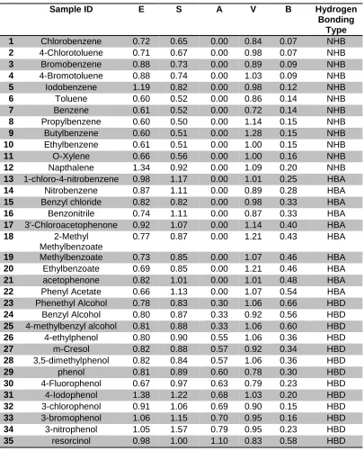
Table 2-1. Solute training set of 35 compounds based on polarity, polarizability, hydrogen
bond accepting, hydrogen bond donating, and size. ... 45
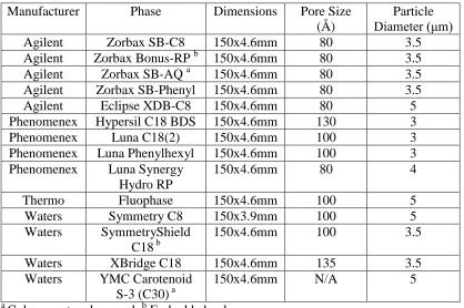
Table 2-2. RPLC stationary phase columns and their physical properties ... 46
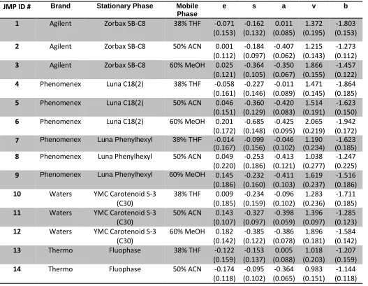
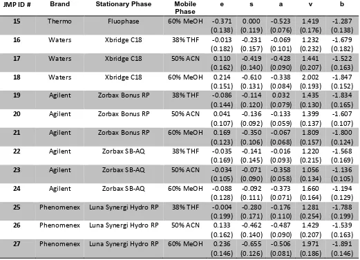
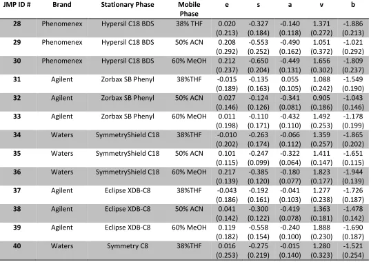
Table 2-3. RPLC system descriptors determined from LSER regression. ... 47
Table 2-4. RPLC coefficient ratios determined from LSER regression. ... 51
Table 2-5. Normalized RPLC system descriptors for the (Xb, Xa, Xs) triangle. ... 53
Table 2-6. Normalized RPLC system descriptors for the (Xb, Xa, Xe) and (Xb, Xs, Xe) triangles. ... 56
Table 2-7. Correlation Matrix of LSER System Parameters for RPLC ... 59
Table 2-8. Eigenvectors for LSER analysis of RPLC systems. ... 60
Table 2-9. Eigenvalues for the five principal components. ... 61
Table 2-10. Variable means and standard deviations after k means clustering for 3 and 4 clusters. ... 62
Table 2-11. LSER descriptors for the sample set selected for validation. ... 63
Table 2-12. k’ data for the validation sample set of 9 RPLC systems. ... 64
Table 2-13. log k’ data for the validation sample set of 9 RPLC systems. ... 65
Table 2-14. Theoretical log k’ data for the validation sample set of 9 RPLC systems. ... 66
Table 2-15. Correlation coefficients for log k’ versus Theoretical log k’ for 9 RPLC systems in the validation of the RST. ... 67
Table 3-1. Peak assignments for ATR-IR spectra for HFIP based on Reference [42]. ... 152
Table 3-2 Changes in the volume of HFIP present in aqueous and coacervate phases of SDS simple coacervate systems with changing the concentration of SDS in the total solution for A) 15% v/v HFIP and B) 25% HFIP in the total solution. ... 153
Table 3-4. Example comparison of the difference between the quantified % w/w HFIP results using the peaks at 1105 cm-1 and 1190 cm-1. The results at 1190 cm-1 artificially increased due to the interference of peaks related to Sodium Dodecyl Sulfate. ... 155 Table 3-5. The % w/w HFIP in the aqueous and HFIP-rich phases in SATPS A) 350mM Na2SO4 and B) 1000mM Na2SO4 ... 156 Table 3-6. Comparison of the water results obtained by GC and the results obtained by Karl Fischer for Na2SO4 systems at constant % v/v HFIP, but changing Na2SO4 concentration in the total solution. ... 157 Table 3-7. Comparison of the water results obtained by GC and the results obtained by Karl Fischer for Na2SO4 systems at constant Na2SO4 concentration, but increasing % v/v HFIP in the total solution. ... 158 Table 3-8. Bromide ion concentration in the aqueous and coacervate phases of DTAB simple coacervate systems. ... 159 Table 3-9. DTA+ concentration in the aqueous and coacervate phases of DTAB simple coacervate systems. ... 159 Table 3-10. Na+ concentration in the aqueous phase and coacervate phases of SDS simple coacervate systems. ... 160 Table 3-11. DS- concentration in the aqueous phase and coacervate phase of SDS simple coacervate systems. ... 160 Table 3-12. Surfactant counter ion concentration in the SDS:DTAB complex coacervate aqueous and coacervate phases. ... 161 Table 3-13. Surfactant concentration in the aqueous and coacervate phases SDS:DTAB complex coacervate system... 162 Table 3-14. DMMAPS concentration in the aqueous and coacervate phase of the zwitterionic simple coacervate system. ... 163 Table 3-15. Na+ and SO42- concentration in the top and bottom phases of the Na2SO4 SATPS. ... 164 Table 3-16. Slope of the correlation between coacervate volume % vs. HFIP% at different [DMMAPS]... 165 Table 3-17. Summary table for coacervate composition as a function of surfactant/salt
Table 4-1. Homogeneity study of the 100mM SDS:CTAB 9% HFIP coacervate phase by comparison of the partition coefficients observed from sampling from the top and bottom of the coacervate... 295 Table 4-2. Results of the equilibration time study on 3 compounds. The partition coefficients changed markedly after 24 hours equilibration, but did not change significantly at 48 hours. ... 296 Table 4-3. Results of a study of the optimal equilibration conditions: vortexing and
centrifuging speed and time. ... 297 Table 4-4. RPLC gradient program for LSER analysis of coacervates. ... 298 Table 4-5A. Compilation of K values for 34 LSER solutes in three Na2SO4 SATPS systems and SDS and DTAB simple coacervates. ... 299 Table 4-6A. Compilation of log K values for 34 LSER solutes in three Na2SO4 SATPS systems and the SDS and DTAB simple coacervate systems. ... 303 Table 4-7. LSER system parameters for the 10 coacervate systems, 3 SATPS systems, and Octanol/Water and their 95% Confidence Intervals. ... 309 Table 4-8. A) LSER coefficient ratios for the 10 coacervate systems, 3 SATPS systems, and Octanol/Water. B) High and low ranges for the coacervate coefficient ratios and MEKC coefficient ratios... 310 Table 4-9. Normalized coacervate system parameters for the ternary plots. ... 311 Table 4-10. 11 MEKC pseudo-stationary phases and their system descriptors.[20, 21, 34] 312 Table 4-11. LSER coefficient ratios for the 10 coacervate systems, 3 SATPS systems,
LIST OF FIGURES
Figure 2-1. RPLC selectivity triangle for 42 RPLC systems using hydrogen bond acidity
(Xb), hydrogen bond basicity (Xa), and dipolarity (Xs). ... 68
Figure 2-2. Plot of RPLC solvent data from Snyder’s SST.[9] 1) Methanol 2) Tetrahydrofuran ... 69
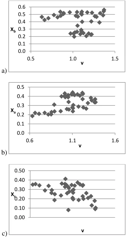
Figure 2-3. Poor correlations between a) Xb b) Xa and c) Xs and v shows that for the RST the X scale is not dependent on the v coefficient. ... 70
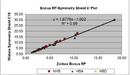
Figure 2-4. k’ plot for Zorbax Bonus RP and Waters SymmetryShield C18 columns with (60:40) methanol: water mobile phase. ... 71
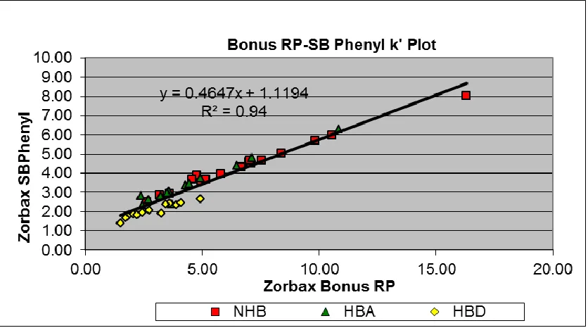
Figure 2-5. k’ plot for Zorbax Bonus RP and Zorbax SB Phenyl columns with (50:50) acetonitrile: water mobile phase. ... 72
Figure 2-6. k’ plot of systems with poor correlation, and distinctively different selectivity. . 73
Figure 2-7. RPLC selectivity triangle for 42 RPLC systems using hydrogen bond acidity (Xb), hydrogen bond basicity (Xa), and polarizability (Xe)... 74
Figure 2-8. RPLC selectivity triangle for 42 RPLC systems using hydrogen bond acidity (Xb), dipolarity (Xs), and polarizability (Xe). ... 75
Figure 2-9. Scatterplot Matrix of the LSER system parameters for RPLC ... 76
Figure 2-10. Loading Plot for principal component 1 versus principal component 2. ... 77
Figure 2-11. Scree plot for principal component analysis. ... 78
Figure 2-12. 3D Plot of the first 3 principal components. The vectors represent the five LSER descriptors. ... 79
Figure 2-13. 3D Plot of the first 3 principal components. The vectors represent the five LSER descriptors. ... 80
Figure 2-14. Score Plot for Principal Components 1 versus Principal Component 2... 81
Figure 2-15. Biplot for principal components 1 and 2. ... 82
Figure 2-16. Dendrogram output from Heirarchical Clustering using Single linkage, and Cubic Clustering Criterion plot. ... 83
Figure 2-18. Dendrogram output from Heirarchical Clustering using Ward linkage, and Cubic Clustering Criterion plot. ... 85 Figure 2-19. Dendrogram output from Heirarchical Clustering using Complete linkage, and Cubic Clustering Criterion plot. ... 86 Figure 2-20. Dendrogram output from Heirarchical Clustering using Average linkage, and Cubic Clustering Criterion plot. ... 87 Figure 2-21. Score Plot of PC 1 versus PC 2 with the 3 clusters from Average linkage
Heirarchical Clustering identified. ... 88 Figure 2-22. Ternary Plot for Xb, Xa, Xs LSER parameters with clusters from hierarchical clustering clusters highlighted (Cluster 1 = black, Cluster 2 = blue, Cluster 3 = red). ... 89 Figure 2-23. Biplot representation of the assignment of the 3 clusters from k-means
Figure 3-5. Phase Diagram for Na2SO4 and HFIP SATPS reported as % HFIP (v/v) and mM Na2SO4 concentration. ... 171 Figure 3-6. The relationship of the % water (w/w) with respect to DTAB concentration in the aqueous phase for 5% v/v HFIP (blue) and 10% v/v HFIP (red) for the DTAB simple
coacervate. ... 172 Figure 3-7. The relationship of the % water (w/w) with respect to DTAB concentration in the coacervate phase for 5% v/v HFIP (blue) and 10% v/v HFIP (red) for the DTAB simple coacervate. ... 173 Figure 3-8. The relationship of % water (w/w) and % HFIP (v/v) for the aqueous phase (red) and the coacervate phase (blue) for 10mM DTAB. ... 174 Figure 3-9. The relationship of % water (w/w) to % HFIP (v/v) for the aqueous phase (red) and the coacervate phase (blue) for 200mM DTAB. ... 175 Figure 3-10. The relationship of the % water (w/w) with respect to SDS concentration in the aqueous phase of the SDS simple coacervate for 15%v/v HFIP (blue) and 25%v/v HFIP (red). ... 176 Figure 3-11. The relationship of the % water (w/w) with respect to SDS concentration in the coacervate phase of the SDS simple coacervate for 15%v/v HFIP (blue) and 25%v/v HFIP (red). ... 177 Figure 3-12. The relationship of % water (w/w) to % HFIP (v/v) for the aqueous phase (red) and the coacervate phase (blue) for A) 10mM and B) 200mM SDS systems. ... 178 Figure 3-13. Plots representing the change in % H2O (w/w) in the aqueous phase of the SDS:DTAB (1:1) coacervate system with respect to the change in total surfactant
concentration for 10% HFIP (blue) and 20% HFIP (red). ... 179 Figure 3-14. Plots representing the change in % H2O (w/w) in the coacervate phase of the SDS:DTAB (1:1) coacervate system with respect to the change in total surfactant
Figure 3-17. Plots representing the change in % H2O (w/w) in the coacervate phase of the DMMAPS simple coacervate system with 10% (blue) and 15% (red) HFIP with respect to the change in total DMMAPS concentration. ... 183 Figure 3-18. Plots representing the change in % H2O (w/w) in the A) 50mM and B) 200mM DMMAPS simple coacervate system with respect to the change in % HFIP (v/v) for
coacervate (blue) and aqueous phase (red) ... 184 Figure 3-19. Plots representing the change in % H2O (w/w) in the aqueous phase of the Na2SO4 aqueous two phase system with respect to the change in total salt concentration for 15% (blue) and 50% (red) HFIP. ... 185 Figure 3-20. Plots representing the change in % H2O (w/w) in the HFIP-rich bottom phase phase of the Na2SO4 aqueous two phase system with respect to the change in total salt concentration for 15% (blue) and 50% (red) HFIP. ... 186 Figure 3-21. Plots representing the change in % H2O (w/w) in the A) 350mM and B)
Figure 3-29. The % w/w HFIP was quantitated by ATR-IR for the coacervate and aqueous phases of the SDS:DTAB complex coacervate systems with A) 5% v/v HFIP in the total solution and B) 10% v/v HFIP in the total solution. ... 195 Figure 3-30. The % w/w HFIP was quantitated by ATR-IR for the coacervate and aqueous phases of the SDS:DTAB complex coacervate systems with changing % v/v HFIP in total solution for A) 50mM total surfactant concentration and B) 300mM total surfactant
concentration. ... 196 Figure 3-31. The % w/w HFIP was quantitated by ATR-IR for the coacervate and aqueous phases of the DMMAPS simple coacervate systems with A) 10% v/v HFIP in the total solution and B) 15% v/v HFIP in the total solution. ... 197 Figure 3-32. The % w/w HFIP was quantitated by ATR-IR for the coacervate and aqueous phases of the SDS:DTAB complex coacervate systems with changing % v/v HFIP in total solution for A) 50mM total surfactant concentration and B) 300mM total surfactant
Figure 3-40. Dependence of coacervate % volume on DTAB concentration for 5% (blue) and 10% HFIP (red). ... 206 Figure 3-41. Change in % coacervate volume with respect to changes in %v/v HFIP for SDS simple coacervates. The trend is a linear increase of coacervate volume with increasing % v/v HFIP. ... 207 Figure 3-42. Dependence of coacervate % volume on SDS concentration for 25% and 45% v/v HFIP solutions. The trend is a linear increase of coacervate volume with increasing SDS concentration. ... 208 Figure 3-43. Changes in % coacervate volume with respect to changes in %v/v HFIP for 100mM and 400mM SDS:DTAB (1:1) complex coacervate systems. ... 209 Figure 3-44. Relationship between coacervate % volume on total surfactant concentration in SDS:DTAB (1:1) complex coacervate systems in 5% and 20% HFIP solutions. ... 210 Figure 3-45. Change in % coacervate volume with respect to changes in %v/v HFIP for DMMAPS zwitterionic simple coacervates for 25mM and 200mM DMMAPS. ... 211 Figure 3-46. Relationship between coacervate % volume on total surfactant DMMAPS for the zwitterionic coacervate systems in A) 5% and B) 10% HFIP solutions. ... 212 Figure 3-47. Changes in % HFIP-rich bottom phase volume with respect to changes in %v/v HFIP for Na2SO4 SATPS: A) 350mM & 1000mM Na2SO4 and B) 100mM Na2SO4. ... 213 Figure 3-48. Relationship between coacervate % volume on total Na2SO4 salt concentration for the Na2SO4 SATPS in A) 35% and B) 50% HFIP solutions. ... 214 Figure A-1. ATR-IR spectrum for 100mM DMMAPS solutions: A) full spectrum and B) expanded window highlighting five DMMAPS-related infrared peaks.. ... 230 Figure A-2. Full spectrum baseline corrected ATR-IR spectrum of 100% HFIP.. ... 231 Figure A-3. Baseline corrected ATR-IR spectrum of 10% HFIP (blue) with 100% HFIP (red). Peak shifting to lower wavenumbers is observed as HFIP concentration increases. Also, peak 11 becomes visible at lower concentrations.. ... 232 Figure A-4. ATR-IR spectrum for 400mM DTAB solutions: A) full spectrum and B)
Figure A-7. ATR-IR spectrum for 500mM Na2SO4 solutions. The peak at 1100 cm-1
interferes with the HFIP bands used for quantitation in the fingerprint region.... ... 236 Figure A-8. Calibration curves for HFIP peaks at A) 1105 cm-1 B) 1190 cm-1 and C) 1285 cm-1. The curve for 1285 cm-1 is not linear and cannot be used for quantitation.... ... 237 Figure A-9. Calibration curves for HFIP peaks in diluted standards for SDS simple
coacervate analysis at A) 1105 cm-1 B) 1190 cm-1 and C) 1285 cm-1... ... 238 Figure 4-1. Chromatogram of Resorcinol with the RPLC method developed for LSER
analysis. Resorcinol is the earliest eluting peak, and is not distorted by diluent/mobile phase mismatch. ... 318 Figure 4-2. The range of values observed for the v parameter in the LSER analysis of 13 coacervate/two phase systems and Octanol/Water. ... 319 Figure 4-3. The range of values observed for the b parameter in the LSER analysis of 13 coacervate/two phase systems and Octanol/Water. ... 320 Figure 4-4. The range of values observed for the a parameter in the LSER analysis of 13 coacervate/two phase systems and Octanol/Water. ... 321 Figure 4-5. Distribution of values observed for the s parameter in the LSER analysis of 13 coacervate/two phase systems and Octanol/Water. ... 322 Figure 4-6. Range of values observed for the e parameter in the LSER analysis of 13
coacervate/two phase systems and Octanol/Water. ... 323 Figure 4-7. Coacervate Selectivity Triangle for 13 coacervate/two phase systems and
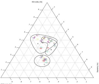
octanol/water using hydrogen bond acidity (Xb), hydrogen bond basicity (Xa), and dipolarity (Xs). This numbering of the systems corresponds to the numbers assigned in Table 4-8. ... 324 Figure 4-8. Coacervate Selectivity Triangle for 13 coacervate/two phase systems and
octanol/water using hydrogen bond acidity (Xb), hydrogen bond basicity (Xa), and
polarizability (Xe). This numbering of the systems corresponds to the numbers assigned in Table 4-8. ... 325 Figure 4-9. Coacervate Selectivity Triangle for 13 coacervate/two phase systems and
Figure 4-22. Plot of log P octanol-water (14) versus log K of 100mM SDS:CTAB 20% HFIP (9). NHB = non-hydrogen bonding, HBA = hydrogen bond acceptor, HBD = hydrogen bond donor. ... 339 Figure 4-23. Plot of log P octanol-water (14) versus log K of 200mM SDS:CTAB 10% HFIP (2). NHB = non-hydrogen bonding, HBA = hydrogen bond acceptor, HBD = hydrogen bond donor. ... 340 Figure 4-24. Plot of log P octanol-water (14) versus log K of 100mM SDS:CTAB 20% HFIP (9). NHB = non-hydrogen bonding, HBA = hydrogen bond acceptor, HBD = hydrogen bond donor. ... 341 Figure 4-25. Plot of log P octanol-water (14) versus log K of 200mM SDS:DTAB 10% HFIP (3). NHB = non-hydrogen bonding, HBA = hydrogen bond acceptor, HBD = hydrogen bond donor. ... 342 Figure 4-26. Plot of log K 100mM SDS:CTAB 10% HFIP (1) versus log K of 200mM SDS:DTAB 10% HFIP (3). NHB = non-hydrogen bonding, HBA = hydrogen bond acceptor, HBD = hydrogen bond donor. ... 343 Figure 4-27. Plot of log K 350mM Na2SO4 25% HFIP (13) versus log K of 100mM
DMMAPS 20% HFIP (11). NHB = non-hydrogen bonding, HBA = hydrogen bond acceptor, HBD = hydrogen bond donor. ... 344 Figure 4-28. Plot of log K 100mM DTAB 10% HFIP (5) versus log K of 350mM Na2SO4 15% HFIP (7). NHB = non-hydrogen bonding, HBA = hydrogen bond acceptor, HBD = hydrogen bond donor. ... 345 Figure 4-29. Plot of log K 100mM DTAB 10% HFIP (5) versus log K of 100mM SDS 25% HFIP (12). NHB = non-hydrogen bonding, HBA = hydrogen bond acceptor, HBD =
hydrogen bond donor. ... 346 Figure 4-30. Scree plot for principal component analysis of coacervate and MEKC pseudo-stationary phases. ... 347 Figure 4-31. Loading Plot for principal component 1 versus principal component 2 for coacervate and MEKC LSER analysis. ... 348 Figure 4-32. Score Plot for PC1 versus PC2 for the coacervates and MEKC pseudo-stationary phases. ... 349 Figure 4-33. Heirarchical Clustering with Single Linkages for MEKC and coacervate
Figure 4-34. Heirarchical Clustering with Centroid Linkages for MEKC and coacervate systems. Cubic Clustering Criterion recommends 19 clusters. Scree Plot recommends 3 clusters. ... 351 Figure 4-35. Heirarchical Clustering with Average Linkages for MEKC and coacervate systems. Cubic Clustering Criterion recommends 19 clusters. Scree Plot recommends 3 clusters. ... 352 Figure 4-36. Heirarchical Clustering with Complete Linkages for MEKC and coacervate systems. Cubic Clustering Criterion recommends 19 clusters. Scree Plot recommends 3 clusters. ... 353 Figure 4-37. Heirarchical Clustering with Ward Linkages for MEKC and coacervate systems. Cubic Clustering Criterion recommends 19 clusters. Scree Plot recommends 3 clusters. ... 354 Figure 4-38. Biplot of the k-means clustering for three clusters. ... 355 Figure 4-39. Score Plot for PC1 versus PC2 for the coacervates and MEKC pseudo-stationary phases, showing the assignment of 3 clusters from Average and Complete linkage
hierarchical clustering. ... 356 Figure 5-1. Unified Selectivity Triangle to compare RPLC and MEKC retention using hydrogen bond acidity (Xb), hydrogen bond basicity (Xa), and dipolarity (Xs). ... 368 Figure 5-2. Selection of RPLC and MEKC systems with similar system parameters, thus similar selectivity. ... 369 Figure 5-3. MEKC electropherogram of 8 solutes, plus methanol as the EOF marker (teo) and decanophenone as the micelle marker (tmc) using 0.04M SDS + 0.4M TFE MEKC in pH 7.0 phosphate buffer as running buffer. ... 370 Figure 5-4. RPLC chromatogram of 8 solutes showing peaks at the retention times shown in Table 5-2 with an Agilent Zorbax SB-Phenyl column and 60% Methanol as the isocratic mobile phase. (DMA= N,N-Dimethylacetamide) ... 371 Figure 5-5. Log k’ correlation between Agilent Zorbax SB-Phenyl column with 60%
CHAPTER 1 INTRODUCTION
Reversed Phase High Performance Liquid Chromatography (RPLC) is a separation technique that uses a polar aqueous mobile phase and a non-polar stationary phase to separate mixtures of compounds. The mechanism of separation in RPLC is based on the partitioning of solutes between the mobile phase and the stationary phase. Separation and elution time may be altered by adjusting the relative polarity of the mobile phase. RPLC has become the leading separation technique for complex mixtures, and is widely used in research and industrial settings. Due to the vast expanse of options related to the stationary phase chemistry, as well as ways to alter the chemistry of the mobile phase, great attention has been drawn to characterizing and classifying both the mobile and stationary phases in order to predict retention.
Micelle Electrokinetic Chromatography (MEKC) was developed by Shigeru Terabe in the 1990s that allows capillary electrophoresis to be used to separate neutral molecules. The mode of separation is similar to RPLC, in that the electroosmotic flow (EOF) behaves similarly to the mobile phase in RPLC, and the micelles are considered a pseudo-stationary phase. EOF forces solutes to migrate toward the detector in the column, while partitioning in and out of the micelles due to the same hydrophobic interactions that affect separation in RPLC. As a result, MEKC and RPLC separation mechanisms are nearly identical, with the same chemical interactions affecting retention and separation.
visualization of the LSER classification of 70 MEKC pseudo-stationary phases.[14, 15]. This work will examine the use of LSER to classify 42 RPLC systems, using 14 RPLC columns and three isoletutropic mobile phases: Acetonitrile: Water (1:1), Methanol: Water (3:2), and
Tetrahydrofuran (THF): Water (62:38). In addition, the concept of the MST will be applied to construct a Reversed Phase Selectivity Triangle (RST) for the visualization and comparison of these systems. Also, multivariate analyses will be used for classification, such as principal component analysis and cluster analysis.
Method Development in RPLC is often a labor intensive task, often requiring the analyst to have many types of stationary bonded phases and mobile phase solvents at their disposal in order to develop a robust and efficient method. The task is extremely time consuming and expensive, and many people have dedicated many years to improving the speed and efficiency of method development procedures. One goal of this research is to combine the MST with the RST into a Unified Selectivity Triangle that will allow the selection of MEKC pseudo-phases with similar retention properties and mechanisms as corresponding RPLC systems. Since the retention mechanisms are similar between these two techniques, we will show that method transfer is possible between MEKC and RPLC. This could prove to be a major breakthrough in the speed and cost of RPLC method development. The cost of MEKC buffers is very inexpensive in comparison to RPLC stationary phases and mobile phase solvents. The ability to develop a method in MEKC and transfer that method to an RPLC system would save in time and money for the method development process.
Coacervates form as two-phase aqueous solutions where amphiphiles in solution are forced to phase separate with the addition of salts[16, 17], pH changes[18], temperature
simple and complex, depending on their composition. Simple coacervates involve a single amphiphile in solution phase separating due to the addition of salt, alcohol, etc. They may also involve two similarly charge amphiphiles that separate based on the repulsion of their charges, and each amphiphile is extracted into separate phases. Complex coacervation is the result of oppositely charge, or catanionic, amphiphiles in solution undergoing a phase transition where one phase is rich in the complex, and the other phase is lean in this complex.
The mechanism for coacervation largely remains unknown; however, coacervation is known to separate and concentrate a large variety of different solutes.[22-25] Partitioning for extraction systems have been characterized by the same LSER that we have used for
classification of RPLC and MEKC systems. In this work, we employed LSER to classify and characterize these simple and complex coacervates. Additionally, we constructed Selectivity Triangles to aid in the visualization of the interactive properties of these systems. Coacervates were also classified using principal component analysis and cluster analysis.
Jenkins discovered perfluoroinated alcohol induced coacervation (PFAIC) while
attempting to modify micelles for MEKC pseudo-stationary phase analysis.[26] Since these types of systems are so closely related, a combined Selectivity Triangle wass developed to compare the selectivity differences in MEKC pseudo-stationary phases and PFAICs. Multivariate analysis was once again used for classification of these systems, using principal component analysis and cluster analysis.
We also performed a full analysis of the chemical composition of the simple and complex coacervates, including phase diagrams, coacervate volume analysis, water analysis, HFIP
References
1. Yang, S.Y. and M.G. Khaledi, CHEMICAL SELECTIVITY IN MICELLAR ELECTROKINETIC CHROMATOGRAPHY - CHARACTERIZATION OF SOLUTE MICELLE INTERACTIONS FOR CLASSIFICATION OF SURFACTANTS. Analytical Chemistry, 1995. 67(3): p. 499-510.
2. Trone, M.D. and M.G. Khaledi, Statistical evaluation of linear solvation energy
relationship models used to characterize chemical selectivity in micellar electrokinetic chromatography. Journal of Chromatography A, 2000. 886(1-2): p. 245-257.
3. Poole, C.F. and T. Karunasekara, Solvent Classification for Chromatography and Extraction. Jpc-Journal of Planar Chromatography-Modern Tlc, 2012. 25(3): p. 190-199.
4. Trone, M.D. and M.G. Khaledi, Characterization of chemical selectivity in micellar electrokinetic chromatography: V. The effect of the surfactant hydrophobic chain. Journal of Microcolumn Separations, 2000. 12(8): p. 433-441.
5. Trone, M.D. and M.G. Khaledi, Characterization of chemical selectivity in micellar electrokinetic chromatography. 4. Effect of surfactant headgroup. Analytical Chemistry, 1999. 71(7): p. 1270-1277.
6. Palmer, C.P., et al., Retention behavior and selectivity of a latex nanoparticle pseudostationary phase for electrokinetic chromatography. Electrophoresis, 2011. 32(5): p. 588-594.
7. Yang, S.Y., et al., Quantitative structure-activity relationships studies with micellar electrokinetic chromatography - Influence of surfactant type and mixed micelles on estimation of hydrophobicity and bioavailability. Journal of Chromatography A, 1996. 721(2): p. 323-335.
8. Yang, S.Y., J.G. Bumgarner, and M.G. Khaledi, Chemical selectivity in micellar electrokinetic chromatography .2. Rationalization of elution patterns in different surfactant systems. Journal of Chromatography A, 1996. 738(2): p. 265-274.
9. Poole, C.F. and S.K. Poole, Column selectivity from the perspective of the solvation parameter model. Journal of Chromatography A, 2002. 965(1-2): p. 263-299.
stationary phases in reversed-phase high-performance liquid chromatography. Journal of Chromatography A, 1997. 766(1-2): p. 35-47.
11. Tan, L.C. and P.W. Carr, Study of retention in reversed-phase liquid chromatography using linear solvation energy relationships - II. The mobile phase. Journal of
Chromatography A, 1998. 799(1-2): p. 1-19.
12. Tan, L.C., P.W. Carr, and M.H. Abraham, Study of retention in reversed-phase liquid chromatography using linear solvation energy relationships .1. The stationary phase. Journal of Chromatography A, 1996. 752(1-2): p. 1-18.
13. Fu, C., Development of Micellar Selectivity Triangle for Classifications of Pseudo-stationary Phase Selectivity in Electrokinetic Chromatography., in Chemistry2005, North Carolina State University: Raleigh, NC.
14. Fu, C. and M.G. Khaledi, Micellar selectivity triangle for classification of chemical selectivity in electrokinetic chromatography. Journal of Chromatography A, 2009. 1216(10): p. 1891-1900.
15. Fu, C. and M.G. Khaledi, Selectivity patterns in micellar electrokinetic
chromatography Characterization of fluorinated and aliphatic alcohol modifiers by micellar selectivity triangle. Journal of Chromatography A, 2009. 1216(10): p. 1901-1907.
16. Man, B.K.W., et al., Cloud-point extraction and preconcentration of cyanobacterial toxins (microcystins) from natural waters using a cationic surfactant. Environmental Science & Technology, 2002. 36(18): p. 3985-3990.
17. Ruiz, F.J., S. Rubio, and D. Perez-Bendito, Tetrabutylammonium-induced coacervation in vesicular solutions of alkyl carboxylic acids for the extraction of organic compounds. Analytical Chemistry, 2006. 78(20): p. 7229-7239.
18. Goryacheva, I.Y., et al., Preconcentration and fluorimetric determination of polycyclic aromatic hydrocarbons based on the acid-induced cloud-point extraction with
sodium dodecylsulfate. Analytical and Bioanalytical Chemistry, 2005. 382(6): p. 1413-1418.
19. Mohanty, B. and H.B. Bohidar, Microscopic structure of gelatin coacervates. International Journal of Biological Macromolecules, 2005. 36(1-2): p. 39-46.
21. Jong, B.d., Colloid Science, ed. H.R. Kruyt. Vol. II. 1949, Amsterdam: Elsevier Publishing Company, INC.
22. Hagarova, I., et al., Coacervative extraction of trace lead from natural waters prior to its determination by electrothermal atomic absorption spectrometry. Spectrochimica Acta Part B-Atomic Spectroscopy, 2013. 88: p. 75-79.
23. Kardani, F., et al., Application of Coacervative Microextraction for Extraction of Volatile Compounds in Thymus Essential Oil and Fruit Juices by Gas Chromatography with Flame Ionization Detection. Journal of Essential Oil Research, 2011. 23(6): p. 61-69.
24. Taechangam, P., et al., Effect of nonionic surfactant molecular structure on cloud point extraction of phenol from wastewater. Colloids and Surfaces a-Physicochemical and Engineering Aspects, 2009. 347(1-3): p. 200-209.
25. Fischer, I., et al., Continuous protein purification using functionalized magnetic nanoparticles in aqueous micellar two-phase systems. Journal of Chromatography A, 2013. 1305: p. 7-16.
CHAPTER 2
Using Linear Solvation Energy Relationships and Reverse Phase Selectivity Triangle for the Characterization of Chemical Selectivity in Reversed Phase High Performance
Liquid Chromatography
Abstract
A selectivity triangle (RST) is developed to characterize the chemical selectivity of 42 Reversed Phase High Performance Liquid Chromatography (RPLC) systems consisting of 14 stationary phases and three isoelutropic mobile phases consisting of Acetonitrile, Methanol, or Tetrahydrofuran and water. The chemical selectivity differences between these systems are determined based on their relative positioning in three ternary plots, where the coordinates are determined based on the relative scales of their hydrogen bond donor ability (Xb), hydrogen bond acceptor ability (Xa), dipolarity (Xs), and ability to interact with lone pair and π electrons. The
RST scheme groups these systems into 3 clusters, organized roughly based on their mobile phase organic modifier type, although a large overlap exists between the methanol based systems and the acetonitrile based systems. Principal component analysis and cluster analysis are also used in conjunction to characterize these systems. Three distinct clusters were found, which roughly agree with the assignment in the RST. Principal component analysis found that all five LSER system parameters are required to give a full characterization of all of these systems. The LSER analysis results were validated for three columns and nine systems in total by using an external solute test set. Experimental log k’ values showed strong correlation with the log k’ values
Introduction
Since its development by Horvath and Lipsky in the late 1960s, high performance liquid chromatography (HPLC) has become the preeminent separation technique in academia and industry.[1-3] Characterization of selectivity in reversed phase HPLC (RPLC) has been of particular interest for many years. To affect selectivity in RPLC, the two most important
variables are the composition of the mobile phase and the type of stationary phase selected. First, selecting the best mobile phase solvent composition has been a large area of focus in the
literature. Researchers have shown that solvents can be classified according to solvent strength and solvent selectivity. Solvent strength is the ability of the solvent to modify retention without changing the relative spacing of the solute bands. Solvent selectivity is the tendency of the solvent to change the relative retention and spacing of the solute bands. The goal in RPLC
method development is to optimize the mobile phase mixture to provide reasonable retention, and sufficient selectivity to separate the solute bands of interest.
the use of the SST to define a process for the optimization of solvent selection to enhance
retention and selectivity. Notably, they outlined the strategy of using solvents found on the apices of the SST to maximize the greatest difference in the type of solvent interactions for both RPLC and normal phase (NPLC). Based on this strategy, the recommended solvents for RPLC were acetonitrile, methanol, and tetrahydrofuran.[6, 7]
Carr and Snyder later showed that the original SST was flawed, in that the test
compounds used were susceptible to more than one of the three interactions. As a result, Snyder redeveloped the SST to use the solvatochromic approach proposed by Kamlet and Taft using dipolarity, hydrogen bond acidity, and hydrogen bond basicity terms that were inherently free effects from multiple interactions.[8] Essentially, this updated SST is very comparable to the original model. As a result, the SST has been adopted as the best qualitative classification of solvents in terms of selectivity.[9]
Linear free energy relationships (LFER) were developed by Kamlet and Taft to
quantitatively characterize physico-chemical and biological processes, where the parameters are derived specifically from Gibbs free energy (ΔG) values. The LFER model was adapted to use solvatochromic properties of solvents, and was referred to as the linear solvation energy
relationships (LSER). LSER has been successfully used as a model for the retention of solutes in various chromatographic techniques.[10-16] The LSER equation can be correlated to different intermolecular interactions and the chromatographic retention parameter k’ as shown below in Equation 2-1:
Equation 2-1.x
donating (HBD) strength or hydrogen bond acidity; S is the solute dipolarity; E is the excess molar refraction. Each solute term has a complementary system parameter. This allows for the full characterization of each molecular interaction and how it affects retention. The system parameters are defined as follows: v is the cohesiveness of the system; b is hydrogen bond acidity; a is hydrogen bond basicity; s is dipolarity/polarizability; e is the ability to interact with n
and π electrons of the solute. The system constant, c, is composed of information about the model
that is not explained the by the five system parameters. When correlated to the retention parameter k’, the phase ratio of the system is the major contribution to this term.[17, 18]
McGowan’s characteristic volume of solute, V, is the energy required to create a cavity
the size of the solute in a solvent. The values for V are calculated by the addition of the atomic volumes of all atoms in the molecule and subtracting 6.56x10⁻⁶ m3/mol, the average bond volume as calculated from water, for each bond, regardless if it is a single, double, or triple bond.
McGowan has calculated these values in m3/mol units for all atoms.[19-22] Excess molar refraction, E, is easily obtained from the refractive index of the molecule, which is an additive property of the individual functional groups.
Solute dipolarity, S, values were determined by gas-liquid chromatography (GLC) retention analysis on five standard polar stationary phases by Françoise Patte and Paul
Laffort[23]. Abraham used these data to construct a new scale for this factor, which is the scale currently used for solvatochromic data analysis. He used an “inverse matrix” method to analyze the original data, along with multiple linear regression using the known GLC column parameters to calculate the solute dipolarity-polarizability values.[24]
Hydrogen bond acidity, Aor2H, values were determined by analyzing the log K for the
related by log K, hydrogen bond acidity and basicity values are all related to Gibbs free energy. A regression was constructed of the log K of the acids versus the log K of the reference base. When the resulting regression lines for different reference bases are plotted in the same chart,
they all tend to intersect at (-1.1, -1.1). Abraham derived an equation for 2H as follows:
2 (log 1.1) / 4.636
H H
A K
Equation 2-2.
Hydrogen bond basicity, B or2H, values were determined in a similar manner where log
K values were calculated for the interaction of bases with a reference acid in the presence of tetrachloromethane. A regression was composed for the log K of the bases versus the log K of the reference acid. As for the acidity plots, the resulting regression lines for differing reference acids all intersect at the “magic point” (-1.1, -1.1). An equation for 2H
was derived as follows:
2 (log 1.1) / 4.636
H H
A K
Equation 2-3.
Commonly, hydrogen bond acidity and basicity values are referenced using the notation Σ2Hand
Σ2H
. This notation reflects the fact that hydrogen bonding interactions are not always 1:1
difference between the complementary interactive properties of the stationary phase and the mobile phase, not a direct measurement of either. The large positive v means that the stationary phase is more hydrophobic than the aqueous mobile phase. A positive e descriptor signifies that the stationary phase is more polarizable than the mobile phase. The negative s coefficient indicates that the stationary phase is less dipolar than the mobile phase. The negative a
coefficient means that the mobile phase is more capable of accepting a proton than the stationary phase. The large negative b coefficient signifies that the mobile phase has much stronger
hydrogen bond donor acidity than the stationary phase.
In RPLC, the mobile phase interacts with the stationary phase and adsorbs onto the surface. This adsorption of water and organic modifier onto the alkyl-bonded silica stationary phase, solvates the chains and unreacted silanol groups on the silica surface that alters the overall interactive properties of the phase.[26-28] Snyder has attributed the increased hydrogen bond basicity of C18 phases after end-capping to adsorbed water on the silica-bonded phase
surface.[29] Adsorption of organic modifiers will also alter the other LSER descriptor properties of the stationary phase, depending on the properties of the organic modifier.
Many researchers have attempted to characterize RPLC stationary phase selectivity using different models. In the late 1970’s, Horavath examined several octadecylsilica columns and
reported their characteristics based on what he termed solvophobic interactions. Differences in solute retention were correlated to phase ratio of the columns, surface tension, polarity of the bonded phase, and dispersion of the bonded phase. In the mid 1980’s, Snyder characterized the
retentivity of fourteen different columns using the retention of 26 compounds in water as well as plotting ln k’ versus ET(30) which is a probe that is used to predict solvent polarity. Column
retentivity is also known as column strength and is generally proportional to bonding phase density and phase ratio.[33]
Cruz et. al. used a combination of the analysis of the chemical properties of the stationary phases and statistical analysis to characterize 30 RPLC columns. These columns were evaluated chemically according to density of alkyl chains (kAB), hydrophobicity (α(CH2)), steric selectivity
(αT/O), hydrogen bonding capacity (αC/P), ion exchange capacity (αA/P) at pH>7, ion exchange
capacity (αA/P) at pH<3, 2,3- and 2,7-Dihydroxynaphthalene efficiency ratio test (DERT),
investigation of metal content, and efficiency. Statistically these columns were evaluated using Principle Component Analysis (PCA) and cluster analysis for the representation of seven-dimensional space.[34]
In 1999, Neue wrote about a procedure Waters Corporation had used to classify silica-based RPLC stationary phases. They determined the stationary phase packing hydrophobicity by obtaining the retention factor for a hydrophobic compound such as acenaphthene. They also considered the selectivity of a pair of basic and neutral compounds, amitriptylene and acenaphthene. These two values were plotted with hydrophobicity (ln k) on the X axis and selectivity of base/neutral compounds (ln α) on the Y axis. This provides a simple visual tool to
choose equivalent phases or very different phases based on their position on the X and Y axes.[35, 36]
claimed to be representative of the broad range of possible solute-solvent interactions.[14, 15, 38, 39] Park and co-workers used LSER to characterize six silica based columns with different bonded phase ligands using a sample set of 24 compounds of widely varying chemical properties.
eE, which accounts for ability of the solute to interact with n and π electrons and excess molar refraction of the phases, was not included in Park’s LSER model. They compared the data
collected on each column for 20% and 40% organic modifier, where the organic modifiers were methanol and acetonitrile.
In the late 1990’s, Tan and Carr released a short series of papers discussing the
applicability of the LSER model to RPLC. However, like Park, they failed to include eE in their LSER equation. The first paper used a sample set of 87 compounds to analyze five columns with different silanol acidity in (50:50) acetonitrile: water to examine the stationary phase
properties.[14] Their second paper used 75 test solutes to analyze one column at 20-50% acetonitrile, methanol, and tetrahydrofuran to examine the mobile phase related properties.[15] They did come to similar conclusion as Park, that the aA and sS terms were of little significance when comparing selectivity in RPLC, while vV and bB were the dominant terms.
In a series of papers beginning in 2002, Snyder and Dolan proposed a new model for the characterization of RPLC stationary phase selectivity called the hydrophobic-subtraction model, which is built on the idea that five solute-column interactions are responsible for selectivity in RPLC.[29, 42-48] These five interactions as represented in Equation 2-4 are hydrophobicity (η’H), steric resistance (σ’S*), hydrogen bonding of acidic solutes with basic column groups (β’A), hydrogen bonding of basic solutes with acidic column groups (α’B), and cation exchange with ionized silanols (κ’C).
The hydrophobic-subtraction model (S-D model) is related to the equation log α = log (k/ kref) = η’H - σ’S* + β’A + α’B + κ’C Equation 2-4.
where η’, σ’, β’, α’, and κ’ are eluent and temperature dependent properties of the solute and H,
S, A, B, and C are eluent and temperature independent properties of the stationary phase. Ethylbenzene is incorporated into the solute test set as the reference solute (log kref) , whose
retention is determined primarily by hydrophobicity. The identities of these terms were derived based on the correlation of the solute and column parameters to the structure of the solutes. The solute parameters were defined such that η’ is solute hydrophobicity, σ’ is molecular bulkiness or the resistance of the insertion of the solute into the stationary phase, β’ is the solute hydrogen bond basicity, α’ is the solute hydrogen bond acidity, and κ’ is the approximate charge on the
solute molecule. The corresponding column parameters were designated as H for hydrophobicity of the column, S* is steric resistance to the insertion of the solute into the stationary phase, A is hydrogen bond acidity of the column due to non-ionized silanols, B is hydrogen bond basicity of the column primarily due to adsorbed water on the stationary phase, and C is column cation exchange activity due to ionized silanol groups. C is a pH dependent term, and has been
except the S* coefficient, which is repulsive. S* has a negative sign in the equation because an increase in the steric resistance to insertion of the solute in the stationary phase will result in fewer interactions, and therefore a decrease in retention.
The S-D method was used to characterize the selectivity of more than 300 RPLC columns.[29, 48] In addition, a column comparison function was developed to demonstrate column equivalence for any two columns:
1
' 2 * * 2 2 2 2 2
2 1 2 1 2 1 2 1 2 1
{[12.5( )] [100( )] [30( )] [143( )] [83( )] }
S
F H H S S A A B B C C
Equation 2-5.
This equation calculates the column selectivity value FS'which is defined as the distance between
two columns, 1 and 2, plotted in five-dimensional space. The weights for each descriptor are the reciprocal of the change allowed in the individual parameter to alter α by 1%. A value of '
S F ≤ 3
can be considered equivalent by this method.
In 2009, Fu and Khaledi reported the characterization of MEKC pseudo-phase selectivity using a novel micellar selectivity triangle (MST), which is conceptually similar to Snyder’s
Fu described a system for scaling the LSER descriptors so that all parameters fall within the range of 0 to 1 using Equations 2-6 to 2-8:
I=i/v Equation 2-6.
low i high low I I U I I
Equation 2-7.
i i
a b S
U X
U U U
Equation 2-8.
where i = a, b, s, or e. This prevents any single coefficient ratio from dominating the effects of the other parameters by normalizing them to the same scale. For Equation 2-7, Ilow and Ihigh are defined as the lower and upper range of the coefficient ratios. Another important note is that the
U terms in the denominator of Equation 2-8 will change based on the apices of the selectivity triangle being used, such that the sum of all Xi for the systems in any selectivity triangle will be
unity. For example, if Xa, Xb, and Xe were the apices, Equation 2-8 would be i i
a b e
U X
U U U
.
Since LSER results for a single micellar phase can vary depending on the lab, sample test set, or different buffer conditions, Fu showed that all 14 SDS systems tested in his lab and from literature converged around the same area when plotted in the MST. This was an important step in proving the viability of using this method for widespread characterization. It is noted,
however, that the best results would come from using the same training set as Fu used to collect the data for the 74 pseudo-phases.
different pseudo-phase clusters have been identified: Group A was comprised of Sodium
dodecylsulfate (SDS) and its analogs; Group B included the strongest hydrogen bond donors and weakest acceptors, consisting of fluorinated micelles; Group C included bile salts,
microemulsions, alkyl methacrylate based polymeric micelles, liposomes, and octanol-water systems; and Group D contained the cationic surfactant TTAB and AGENT polymeric micelles. MST for the other two options showed the same type of clustering with the four distinct groups. The MST chosen for further analysis was the (Xb, Xa, Xs)due to the better separation of the 4
groups, and the compatibility with Snyder’s SST. Fu concluded that the MST model is useful for
the characterization and rational selection of pseudo-phases for the optimization of MEKC separations.[49]
Zhang and Carr used Fu’s approach to the MST to construct a stationary phase selectivity
triangle based on the S-D method. They used a shortened approach to this method, using a training set of 10 solutes for the testing of type B alkyl silica columns, and a set of 18 solutes for other types of columns. This shortened version was shown to give accurate results compared to the larger sample set used to build the model for the ACN based systems. The same
normalization approach was used as in the MST, where all of the terms were converted to
coefficient ratios by dividing by the hydrophobicity term, H, then normalized based on Equations 2-6 to 2-8. Four triangles were created using different combinations of the parameters Xa, Xb, Xs,
and Xc as the apices. The triangles were (Xs, Xb, Xc), (Xs, Xa, Xc), (Xa, Xb, Xc), and (Xs, Xa, Xb).
In this study, 366 stationary phases were characterized on all four selectivity triangles using 50:50 ACN: water mobile phase, buffered at pH 2.8 using 30mM phosphate buffer. As a result, the C coefficient in this analysis was C(2.8) only. “Extreme phases” were noted that spanned a
marked as possible orthogonal columns, and tests showed that for certain solute mixes, this was the case. The “extreme phases” consisted mostly of phases with embedded polar groups or using
stationary phase supports other than high purity silica. The analysis of all four triangles
concurrently was recommended to properly characterize the selectivity of stationary phases for RPLC.[51]
Analysis of the LSER parameters and ternary plots alone cannot help with determining the optimum number of variables needed to fully characterize the model, or to what extent each variable affects solute partitioning. Two multivariate analyses are commonly used for this type of classification: principal component analysis and cluster analysis. These two chemometric
methods are very powerful tools for processing large data sets that are inter-correlated and
multidimensional, and each has its own strengths and weaknesses. Used in conjunction, these two methods can provide clear visual and quantitative data to justify the number of variables used for characterization, and the influence of each variable on retention.
Principal component analysis (PCA) is a statistical method for reducing the
dimensionality of a data set with a large number of highly correlated variables, while retaining as much variance in the data set as possible. This is accomplished by creating a new, smaller set of uncorrelated variables, where the first few variables preserve most of the variance from all of the original variables. These new variables are the principal components (PCs). In the current data set, we have a data matrix X, with m x ndimensions, where m is the number of RPLC systems, and n is the number of LSER variables that describe the RPLC systems. The data are adjusted by subtracting the mean from each dimension, which yields a data set with a mean centered at zero in matrix Xc. As a result, the covariance matrix S of the data can be written as follows:
where T is the transpose of the matrix. Since the matrix is a square 5x5 matrix, it is possible to calculate eigenvalues and eigenvectors using Single Value Decomposition (SVD). SVD can be written here as follows:
Equation 2-10
where U is an m x m square matrix that consists of the principal components, Σ is an m x n diagonal matrix where the nonzero values are the square root of the eigenvalues, and VT is a n x n square matrix and the n columns of VT are the eigenvectors. Finally, the principal components matrix z can be written as:
Equation 2-11
The eigenvalues can be ordered from highest to lowest, which will place the components in order of significance based on their variance. The first principal component always explains the largest variance in the data.[52]
Cluster analysis is another multivariate method for characterizing RPLC systems. Cluster analysis attempts to place the data into groups where the members of the groups are similar with respect to their variables, and the clusters themselves are distinctive. Linkages and similarities are evaluated based on their inter-point distances. JMP is a visual data analysis software package created by SAS, and will be used here for multivariate analyses. Five linkage types are are available for comparison: Average, Centroid, Ward, Single, and Complete. Average linkage uses the average distance between pairs of observations, one in each cluster. The distance is calculated as:
where DKL is the distance between the observations in clusters CK and CL, CK is the Kth cluster,
d(xi, xj) is the Euclidian length of the vector x, and NK is the number of observations in CK.
Centroid linkage uses the squared Euclidian distance between the means of the clusters to calculate distance:
‖̅ ̅ ‖ Equation 2-13
where ̅ is the mean vector for cluster CK.
Ward clustering seeks to minimize the variance of the cluster being merged by using the ANOVA sum of squares using the following equation:
‖ ̅ ̅ ‖
Equation 2-14
Single clustering uses the “nearest neighbors” from the clusters to calculate the minimum
distance between the clusters, where the distance equation is:
Equation 2-15
Complete clustering uses the maximum distance between the elements of the clusters, or the “farthest neighbors,” where the distance equation can be quantified as:
Equation 2-16
Since each of these options can produce very different results, criteria must be set to determine the optimal linkage method and the appropriate number of clusters needed to accurately represent the data. Two methods exist in JMP to determine the appropriate number of clusters for each linkage method. First, a Scree Plot can be seen beneath each dendrogram which plots the number of clusters against the distance for each cluster. Using the “elbow” method described for the PCA
determine the ideal number of clusters for the data, by looking for the largest CCC value. A CCC value greater than 3 indicates that the clustering is a good fit, and higher values mean a better fit.
Two methods of clustering analysis are available that will provide orthogonal analysis of the data. Hierarchical clustering is a “bottom up” approach where each point begins as its own
cluster. The distance between each cluster is then calculated and the two closest clusters are combined to form a new cluster. This continues until all of the data points are in one large cluster. The cluster are represented in a dendrogram, which is a tree-like structure, and the clustered data points are connected by inverted U-shaped links called the fusion of the data points. The height of each U bar represents the similarity of the data points being clustered. Shorter height means more similarity exists between fused data points. Using the dendrogram, the user can then determine the optimal number of clusters for the given model.
In contrast, k-means clustering is a “top down” approach to clustering. k-means is an iterative process where the data points are fitted to a predetermined number of clusters. The data points are then clustered based on their distance from the centroid of each cluster. This process is repeated until the sum total of the distances is at a minimum and no changes are seen in the clusters.
cluster analysis to characterize gas chromatography stationary phases.[65] These chemometric methods have also been widely employed for characterization of the complex chemical
interactions that affect partitioning in high performance liquid chromatography (HPLC). Carr et. al. have used PCA and LSER to model retention for many HPLC stationary phases. In one study, they evaluated alkyl, aromatic, and fluorinated stationary phases and showed that PCA was more accurate than LSER in prediction of solute retention, but PCA failed to explain all the data in the three classes of bonded phase[66].
In this chapter, linear solvation energy relationships are used in conjunction with ternary plots to characterize 42 unique stationary phase and mobile phase combinations for
characterization in RPLC. Additionally, principal component analysis and cluster analysis are applied as multivariate analyses to reduce the dimensionality and the number of correlations in the data to model retention in these systems.
Experimental Section Materials
All data were collected on an Agilent HP1100 HPLC system with a binary pump and a multiple wavelength UV-Vis detector. The detector was used at a wavelength of 254nm, the column temperature was controlled at 25°C, and the mobile phase flow rate was 1.0mL/min. Uracil was used to provide a peak to represent the void volume of the system for calculating the capacity factor. Retention times for the peaks were recorded at the peak maximum using Waters Empower version 2.0 or Thermo-Electron Atlas version 8.1.
Jersey). The solutes were diluted in a 25mL volumetric flask with methanol to a level where the peaks were visible and able to be integrated by the software. A standard solution was prepared that included uracil, to mark the void volume, and benzyl chloride. The standard was injected at the beginning, middle, and end of the chromatographic sequence to determine the suitability of the HPLC system based on %RSD ≤ 1.5% of the peak retention times (RT). Data calculations
and linear regression analysis were performed using Microsoft Excel 2010. Ternary plots of the data and multivariate analyses were performed using JMP 10.0 made by SAS Institute.
Methods
A training set of 35 solutes varying in polarity, polarizability, hydrogen bonding ability, and size were carefully selected as listed in Table 2-1. The test solutes were run on 14 columns varying by manufacturer and type of bonded phase, which are listed in Table 2-2. To maintain the same solvent strength, each column was run with isoelutropic mixtures of the three common hydro-organic mobile phases: 50:50 ACN: water, 60:40 MeOH: water, and 38:62 THF: water. These mobile phase and stationary phase combinations have resulted in 42 different RPLC systems to classify using the LSER model. This experimental design will prove to characterize the complete interaction between the solute, the mobile phase, and the stationary phase.
Results and Discussion
Linear Solvation Energy Relationships for RPLC Systems
MEKC). LSER is used here to characterize 42 different RPLC systems. The LSER regression was run on these systems, given the LSER solute descriptors in Table 2-1. The samples in Table 2-1 are divided into three distinct groups based on their hydrogen bonding characteristics: hydrogen bond donor (HBD), hydrogen bond acceptor (HBA), and non-hydrogen bonding (NHB) for comparison of RPLC systems based on selectivity of solutes with different hydrogen bonding properties.
The calculated solute retention factor (k’) values from the chromatographic sequences according to Equation 2-17:
' R 0
R t t k
t
Equation 2-17.
where tR is the retention time of the solute of interest, and t0 is the void volume of the system as
measured by the retention time of uracil. The coefficients of the regression are the five system descriptors: v, b, a, s, and e, and are calculated based on the LSER regression for the 42 RPLC systems. The calculated parameters are compiled for each system in Table 2-3. LSER
Selectivity triangles have successfully been used over the years to classify the selective properties of LC solvents, mobile phases, and stationary phases.[9] Fu used selectivity triangles to classify 74 MEKC pseudo-phases.[49] Zhang and Carr followed up by using Fu’s scheme for normalization and selectivity triangle characterization for RPLC columns using the S-D
model.[51] As a result of the recent success, a selectivity triangle scheme was selected to characterize the 42 RPLC systems reported here using LSER. Because of the difference in the directionality of the axes used by Snyder, the RPLC mobile phase solvents were plotted using the directionality of the axes used in this research, as shown in Figure 2-2 for ease of comparison.
First, the RPLC system descriptors from the LSER analysis were converted to coefficient ratios via Equation 2-6, by dividing each system coefficient by the hydrophobicity term (vV), as shown in Table 2-4. The X terms should not be dependent on the v coefficient. The poor
correlations shown in the plots in Figure 2-3 confirms that the X scale is independent of the magnitude of the v coefficient.
The normalized RPLC system descriptors, as calculated from Equations 2-7 and 2-8 can be found in Table 2-5. Using this data, an RST was developed based on Snyder’s solvent
selectivity triangle and Fu’s MST using hydrogen bond donor acidity (Xb), hydrogen bond donor
basicity (Xa), and dipolarity (Xs) for all 42 RPLC systems (Figure 2-1). In general, the systems
![Figure 2-2. Plot of RPLC solvent data from Snyder’s SST.[9] 1) Methanol 2) Tetrahydrofuran 3) Acetonitrile 4) Water](https://thumb-us.123doks.com/thumbv2/123dok_us/1265936.1159175/94.612.94.532.83.454/figure-plot-solvent-snyder-methanol-tetrahydrofuran-acetonitrile-water.webp)