HEINTZE, OLAF. A Computationally Efficient Free Energy Model for Shape Memory
Alloys - Experiments and Theory. (Under the direction of Dr. Stefan Seelecke.)
Shape memory alloys (SMA) belong to the class of active materials and have recently
been considered as novel actuation and damping mechanisms in micro- and macro-scale
applications. Combined with their advantageous lightweight and high work output
char-acteristics is a complex, highly non-linear and hysteretic material behavior, which is also
thermo-mechanically coupled. Due to this complexity, model development for SMA material
behavior is a challenging task, and experimental data in particular about the inner
hystere-sis loops is necessary to gain further understanding and successfully design applications. In
this thesis, a single crystal material model is presented and subsequently extended to the
more realistic polycrystalline case considering material inhomogeneities, grain impurities
and lattice imperfections. A first implementation, based on a stochastic homogenization procedure, provides a very accurate description of the observed phenomena, but also
re-quires very high computation times. A reformulation of the underlying concept leads to a
parameterization method, which preserves the advantages of the original method, but
dra-matically reduces the computation times. It is shown that the material behavior prediction
of both models are identical, and the parameterization method is compared extensively to
data from tensile experiments with a pseudoelastic SMA wire. Remarkably, the model is
able to capture all facets of the material behavior including rate-dependence and minor
loops. The versatility of the model also allows for the simulation of SMA actuator behavior
including the electrical resistance. Finally, a MEMS device using polycrystalline SMA thin
film actuators is experimentally investigated. As a first step, the material behavior of the SMA thinfilms is presented using strain-temperature and resistance-temperature measure-ments. Secondly, the performance of the MEMS device was determined for different driving
FOR
SHAPE MEMORY ALLOYS - EXPERIMENTS AND THEORY
by Olaf Heintze
a dissertation submitted to the graduate faculty of north carolina state university
in partial fulfillment of the requirements for the degree of
doctor of philosophy
department of mechanical and aerospace engineering
raleigh December 2004
approved by:
Peter
Ursula and Erich
In memoria
Olaf Heintze saw the light of day after a breathtaking car chase on January 24, 1975 on the eastern side of the German Wall in the city of Dessau. As a son of two high school
teachers for the most beloved school subjects, namely mathematics, physics, chemistry
and astronomy, a future career in engineering seemed to be already unavoidable at this
point. He spent his childhood in Oranienbaum, Germany, whether behind the counter of
his grandparents hardware store or in the physics lab of his parents school. He learned
summating prices in the hardware store and setting up electrical circuitries in the physics
lab, which became handy later on during his time in school.
Guided by the roots of his childhood, he earned the degree Diplom-Ingenieur from
the Technical University in Berlin in Physical Engineering Science in 2001 and had been
generously offered to enroll in a Ph.D. program abroad. Following this offer, he became
a Ph.D. student at the Mechanical and Aerospace Engineering Department of NC State
University in the very same year.
I would like to extend my deepest gratitude to my advisor and founder of my research
career Prof. Dr.-Ing. Stefan Seelecke. Since we started working together in Berlin in 1999,
I realized how much I still have to learn about profound, real-world engineering and that
he would be the one to learn it from. I sincerely thank you for the support and guidance
during all those years as well as for the generous offer to become your Ph.D. student and,
thus, allowing me to widen my experience enormously. Danke.
For being always helpful, encouraging and supportive, I would like to thank my
com-mittee members Dr. Mohammad Noori, Dr. Ralph C. Smith and Dr. Richard F. Keltie.
Although the air was often on fire and time always precious, you managed to be available for me. Thank you, Dr. Keltie, for your advise and engagement, when I needed it the
most.
I also would like to thank Dr. Gould for his fast and uncomplicated help during all my
time in the Ph.D. program.
Dr. Shaw. Thank you so much for providing me with access to your wonderful lab.
You even have colored screw drivers! I especially enjoyed your profound way of conducting
research combined with your great sense of humor. I also still miss the Fragles.
Many thanks to the staff of the MAE department, especially to Betty, who always
answered calmly my questions and to Mike and Skip, who always did their best to make
my experiments happen.
Although, they have left this university already, I need to thank my former fellow
stu-dents Jason and Jinghua for the scientific discussions we had and for introducing me to
their own cultures.
The NC State Water Polo Club. What had I done without you guys? You allowed me
Yuriy for being my friends and for giving me the final boost, when I started to loose it. Another great ’thank you’ goes to the three T’s. Thanks Tim and Tim for the endless
discussions we had. Big thanks also to my room mate Tom. Chief, I’ll never forget your
help and encouragement.
The last and greatest Danke goes home to my family in Germany. You always
sup-ported me and made all this happen by your strong commitment to this little family and
to education. Although I can’t thank many of you in person anymore, I’m confident that
it reaches you.
List of Figures viii
1 Introduction 1
1.1 Motivation and Background . . . 1
1.1.1 Applications . . . 1
1.1.2 Modeling . . . 2
1.2 Thesis Objective . . . 7
1.3 Thesis Outline . . . 8
2 Perfectly Homogeneous Single Crystal Model 10 2.1 Assumptions . . . 10
2.2 Free Energy as Central Quantity . . . 12
2.3 Stress-Strain Relation . . . 15
2.4 Kinetics of Phase Transformation . . . 16
2.5 Balance of Internal Energy . . . 20
2.6 Summary of Model Equations and Simulation of Hysteresis Loops . . . 21
3 Inhomogeneous Polycrystal Model - Direct Implementation 24 3.1 Concept of Stochastic Homogenization . . . 24
3.1.1 Stress vs. Strain Control . . . 27
3.1.2 Convergence Analysis . . . 30
3.1.3 Effects of Distribution Parameters . . . 34
4 Parameterization Method - Representative Single Crystal 37 4.1 Concept of Parameterization . . . 37
4.1.1 Parametrization Method for a Single Distribution . . . 38
4.1.2 Parametrization Method for Two Combined Distributions . . . 42
4.2 Implementation Details . . . 49
4.3 Evaluation of Parameterization Method . . . 52
4.3.1 Comparison with Direct Implementation . . . 53
4.3.2 Comparison with Experimental Data . . . 55
4.3.3 Simulation of Sensor and Actuator Behavior . . . 62
5 SMA MEMS Actuator Experiments 67
5.1 Introduction . . . 67
5.2 Material Properties . . . 68
5.2.1 Setup and Procedure . . . 68
5.2.2 Mechanical and Sensor Properties . . . 70
5.2.3 Conclusions . . . 80
5.3 Actuator Performance . . . 80
5.3.1 Procedure and Setup . . . 80
5.3.2 Open Loop Results . . . 81
5.3.3 Conclusions . . . 83
6 Conclusions 85
List of References 87
2.1 Lattice particle of a shape memory alloy in its possibel phases autenits A
and martensite M±. . . 10
2.2 Typical layer structure. . . 11
2.3 Layer model of a macroscopic material . . . 12
2.4 Free energy of a lattice layer for a fixed temperature without (left) and with external load (right). . . 13
2.5 Free energy of a lattice layer for different temperatures. . . 14
2.6 Free energy for a lattice layer forT = 328K and different loads. . . 15
2.7 Isothermal, mechanical response of a single crystal SMA for different temper-atures. Quasi-plastic (left, T = 280K), transition to pseudo-elastic (middle, T = 308K), and pseudo-elastic material behavior (right, T = 338K). . . 22
2.8 Strain vs. temperature behavior for two different loads. . . 23
3.1 Effect of distribution in barrier (left) and internal stress (right). . . 25
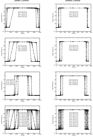
3.2 Comparison of strain and stress control for 9 integration points. . . 29
3.3 Comparison of strain and stress control for 9 integration points. Phase frac-tion evolufrac-tion. . . 31
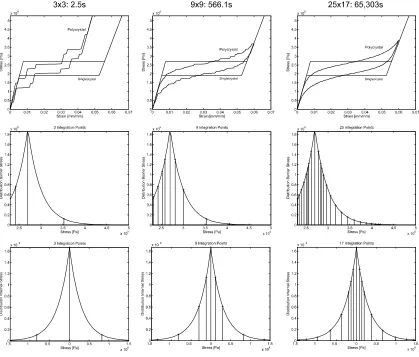
3.4 Convergence behavior for isothermal tensile experiment. . . 32
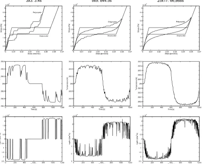
3.5 Convergence behavior for non-isothermal experiment. . . 33
3.6 Pseudoelastic material behavior due to different distribution combinations, 1st order reversal . . . 35
3.7 Pseudoelastic material behavior due to different distribution combinations, 2nd order loops . . . 36
4.1 Gibbs free energy landscape during loading/unloading for elements with dif-ferent energy barriers. . . 40
4.2 Normal Distribution of barrier stresses and associated phase fraction change. 41 4.3 Gibbs free energy landscape during loading/unloading for elements with dif-ferent interaction stresses. . . 43
4.4 Gibbs free energy landscape during loading/unloading for elements with dif-ferent energy barriers and interaction stresses. . . 44
4.5 Contour and surface plots of double-distribution landscape during intial load-ing process. . . 47
4.7 Numerical evaluation of double integral to calculate the phase fraction . . . 50
4.8 Phase transformation probabilities for single crystal SMA. . . 52
4.9 Phase transformation probabilites for parameterized SMA model. . . 53
4.10 Comparison of parameterized model and direct implementation, isothermal case. . . 54
4.11 Comparison of parameterized model and direct implementation, non-isothermal cases (strain rates 1e-4, 1e-3, 1e-2 1/s). . . 56
4.12 Isothermal case with barrier from data . . . 57
4.13 Strain rate effect - data and parameterized model . . . 58
4.14 Major loops - comparison with data for different strain rates. . . 59
4.15 Partial loading - comparison with experimental data for different strain rates. 60 4.16 Partial unloading - comparison with experimental data for different strain rates. . . 60
4.17 Minor loops - comparison with experimental data for different strain rates. 61 4.18 Relaxation - comparison with experimental data for different strain rates. . 62
4.19 Actuator properties for different loads - major loops . . . 64
4.20 Actuator properties for different load - partial heating. . . 65
4.21 Actuator properties for different loads - partial cooling . . . 65
4.22 Actuator properties for different loads - minor loops. . . 66
5.1 MEMS device; Schematic sketch (left), DMA7efixture (middle), 1-steel base, 2-stamp, 3-PC board, 4-lead wires, device after testing (right) . . . 69
5.2 Geometrical constraints due to MEMS principle of operation. . . 70
5.3 Major loops. Strain vs temperature (top), resistance vs temperature (bot-tom) for increasing load (left to right). . . 72
5.4 Partial heating, 1. type. Strain vs temperature (top), resistance vs temper-ature (bottom) for increasing load (left to right). . . 74
5.5 Partial heating, 2. type. Strain vs temperature (top), resistance vs temper-ature (bottom) for increasing load (left to right). . . 75
5.6 Partial heating. Temperature vs. time (left), strain vs. temperature (middle) and resistance vs. temperature (right). . . 76
5.7 Close up picture of MEMS device after testing with textured SMA actuators. In and out of plane deformations along SMA strips. . . 77
5.8 Partial cooling. Strain vs temperature (top), resistance vs temperature (bot-tom) for increasing load (left to right). . . 78
5.9 Minor Loops. Strain vs temperature (top), resistance vs temperature (bot-tom) for increasing load (left to right). . . 79
5.10 MEMS performance testing device . . . 81
5.11 MEMS actuator performance for 0.5Hz, 5Hz and 10Hz electric current input (rectangular pulse). . . 82
Introduction
1.1
Motivation and Background
The shape memory phenomenon has been known for about seventy years now, but did not
receive much attention since its discovery by Ölander (see [64], [65]). It was rediscovered
by Bühler (see [22]) in the 1960’s, and technical applications are pursued since then.
After plastic deformation at low temperature, a shape memory alloy (SMA) restores its
initial configuration upon the supply of heat. This ’memory’ of the original shape provided
the name for the effect. At a higher temperature, the material exhibits another behavior.
Here the material can be reversibly deformed up to10%of its original length under a nearly constant load. This effect is called superelasticity. Both effects are a consequence of the
quasiplastic and pseudoelastic load-deformation behavior at low and high temperatures,
respectively. The underlying mechanism is a phase transformation between different
crys-tallographic structures, i.e. different variants of martensite and the austenite phase. Details
about the material behavior can be found in the textbooks of Funakubo [26] and Otsuka
and Wayman [67].
1.1.1
Applications
Some of the early applications were pipe couplings and electric circuit breakers acting
au-tonomously to changes in the environmental temperature. Due to their biocompatibilty,
they also found their way into medical applications. They cover the range from self-adjusting
braces to tubular, self-expanding stents. Although they have also been used for energy
con-version purposes (see Glasauer and Müller [28]), two main application areas are damping
mechanism and actuation. Thefirst one is made possible by the non-linear hysteretic ma-terial behavior causing energy to dissipate. In particular, this is useful for the damping of
civil structures that need an efficient seismic isolation or a protection against wind
vibra-tion. For most recent applications see Wildeet al [82], Aizawaet al [5] and DesRoches and
Delemont [24]; for modeling of hysteresis-induced damping behavior see Seelecke [71] and
[72].
Since shape memory alloys provide the highest work output of all known actuation
mechanisms combined and are lightweight (see Hollerbachet al [38]), they are an attractive
choice for actuator applications. This ranges from macro-scale applications like adaptive
wing shape control (Bauer et al [6],Breitbach et al [19],Hanselka et al [35],Kudva et al
[53] and Campanile et al [23]). Campanile et al [23] use SMA actuators below the flexible surface of a trailing edge to control the position of transonic shocks. In addition to aerospace
related applications, SMAs are also used in robotics. Vaidyanathan creates a worm-like
robot (see [80]), and a controlled six-legged robot is presented by Heintze [36]. Other
robotic applications are, e.g., multifingered hands (Schleich [69])
The most promising area for SMA actuators is the field of micro-electro-mechanical systems (MEMS). Since the SMA actuation mechanism relies on passive cooling, their
effectiveness increases with decreasing dimensions. Micro-scale actuators have large surface
to volume ratio and, thus, effective cooling even when surrounded by still air. Hoet al [37]
report a thinfilm micropump operating at a frequency of300Hz. Such micropumps are used in microfluidics in, e.g., medical drug dosage systems and ink jet printers. A related area is
microvalves as presented by Kohl et al ([52], [50]). A US-based company, TiNi-Alloy, even
has a commercial product available, see Johnson [46], [48]. In [47] Johnson also explains in
the advantages of SMA MEMS actuators simultaneously claiming the lack of available data
and systematically conducted experiments, which provided one motivation for this work.
1.1.2
Modeling
If one wants to make an efficient use of these novel applications and successfully
thermomechanically-coupled material behavior of shape memory alloys.
Early efforts go back to Tanaka and Nagaki [79], [77] and [78]. The model uses the
fraction of martensite as an internal variable and gives a phenomenological equation of
state for its dependence on stress and temperature in the form of an exponential function.
It provided the basis for a related model suggested by Liang and Rogers [55], who found
a cosine law for the martensite fraction to be more convenient. However, both versions
were only applicable to the high temperature case of pseudoelasticity, and it was only
after Brinson [20] introduced a decomposition of the martensite fraction into twinned and
detwinned martensite, that the quasiplastic behavior could be described as well. Due to
the phase diagram necessary to distinguish between the different branches of the martensite
fraction equation, these models are also called state-space models, see Bekker and Brinson
[7] for a generalization of the concept. All these models are purely mechanical in the sense
that temperature is considered as a parameter.
Boyd and Lagoudas [18] have developed a model that is derived from irreversible
thermo-dynamics. Based on the second law, an ansatz for the entropy production is made resulting
in an evolution law for the phase fractions which is thermodynamically admissible. The
model follows the guidelines of the classical theory of rate-independent plasticity with yield
conditions triggering the phase transformations and is formulated in a three-dimensional
setting. Closed form solutions for damping capacity and actuator efficiency are obtainable
from the model. A drawback, however, is the large number of material parameters to be
determined. Furthermore, due to its provenance from the classical theory of plasticity, the
dissipation potential is not chosen from physical reasoning but rather from mathematical
arguments like convexity properties.
Recently, a number of articles have been published, which attempt to combine the
framework of irreversible thermodynamics with a more detailed study of the underlying
microstructure. The main objective is to find a suitable expression for the free energy as composed of chemical and mechanical parts. The chemical part is temperature dependent
and is mainly determined by the entropies of austenite and martensite, whereas the
me-chanical contribution is due to the stress and strain fields from external loading and the interaction between the different phases. This interaction is due to the strains associated
driving force for the transformation is calculated and set equal to dissipative terms from
interfacial energy contributions and so-called internal friction. Thus, an equation is derived
for the evolution of appropriate martensite phase fractions. Models of this type have been
proposed by several authors, among them Lu and Weng [56], who give a single crystal
for-mulation for oblate inclusions, which they extend to a self-consistent model for polycrystals
in a subsequent paper, [57]. A similar approach has been taken by Huang and Brinson [39],
who first illustrate the procedure for a fictitious two-variant material and later extend it to a typical 24 variant case. While in this paper the authors treat spheroidal inclusions,
they turn to the more realistic case of penny-shaped inclusions in Gao et al [27]. Here,
they also introduce a distinction between habit plane variants and correspondence variants,
accounting for the fact that habit plane variants may consist of smaller subunits leading
to an internal structure in the form of a certain stacking sequence. This model is further
generalized to polycrystalline behavior, see Gao Etal [40]. Bo and Lagoudas [13, 14, 15,
16] also present a paper on a polycrystalline model of such type, consisting of four parts.
Their main focus is on the introduction of plastic strains, which is an important mechanism
present in some SMAs under cyclic loading applications. It is shown to lead to a degradation
of performance when a non-stabilized material is used in an actuatoric application. The
authors use back and drag stress as internal variables and are able to simulate the two-way
shape memory effect, which is also related to the evolution of plastic strains. After a
the-oretical derivation of the three-dimensional formulation in part I, a material undergoing a
stable transformation cycle is treated in part II in a one-dimensional setting. This version
is also used for the full plastic model which is compared to experimental results in part
III. Part IV discusses the relationship to so-called Preisach models often used by hysteresis
researchers with a mathematical background. The model’s capabilities with respect to the
simulation of internal hysteresis loops are demonstrated.
Lagoudas and Entchev continued this work in [54] and further applied this model to
porous SMAs in [25]. Khanet al [49] present a Preisach model pseudoelastic response that
can model minor hysteresis loops, but does not consider the strain rate effect. Both models
are able to simulate polycrystalline material behavior.
Another recent model based on micromechanical considerations has been proposed by
Lexcellent [81], who study the differences between tension and compression in
pseudoelas-ticity. Bouvetet al [17] present a model considering the same differences and incorporating
multiaxial proportional and nonproportional loading. It considers rate-independent
plastic-ity and minor loops due to yield surfaces for the phase transformation as a function of the
phase fraction.
Novak and Sittner present a micromechanical modeling approach for polycrystalline
SMA in [62],[63].
The authors in [21] propose a phenomenological model for polycrystalline SMA, based
on statically constrained micro-plane theory. Hereby, the macroscopic material behavior is
obtained by the evaluation of stresses and strains on differently oriented microplanes. The
paper presents simulations of polycrystalline material behavior based on 28 microplanes.
This approach can model minor hysteresis loops, and the ones shown for uniaxial loading
close after intensive cycling. It is expected from experiments and theory that minor loops
close only for the isothermal case. Since the model incorporates changes in temperature, a
discussion of the strain or stress rate effect would be desirable to explain the phenomenon
of non-closing minor loops.
The state-space models discussed above may be regarded as the beginning of SMA
modeling, and they are still nowadays widely used among engineers due to their conceptual
simplicity. Their suitability for the simulation of actuator applications, however, is very
limited. The same holds for the recent micromechanical models discussed above, which,
although possessing a high level of sophistication, are far too complex to be used for the
simulation of mostly one-dimensional SMA actuators. Here, in the present paper, the
major concern is a good one-dimensional description accounting for both, thermodynamic
and mechanical aspects, at the same time offering the possibility of implementation into
advanced control algorithms.
A noticeable model in this respect has been developed by Ivshin and Pence [44, 45].
The authors perform a detailed thermodynamic analysis to motivate their basic equations.
The potential of thermodynamic analysis, however, has not been fully exploited as it only
deals with the case of equilibrium thermodynamics based on integrability conditions derived
description of the hysteretic shape memory behavior. They enter the model through
so-called envelope functions resulting in an ordinary differential equation of Duhem-Madelung
type for the austenite phase fraction. Despite a certain lack of physical reasoning, the
model appears to be quite powerful with respect to the simulation of actuatoric behavior.
It includes an energy balance with contributions from convective heat exchange, latent heats
and external heat sources, and a number of interesting simulations are displayed in [45].
Ikeda et al [43] introduce a macroscopic model for uniaxial loading derived from a
grain-based microscopic model. They have incorporated an energy balance and are able
to model inner hysteresis loops. The phase transformation occurs by exceeding a required
transformation energy, which is derived with arguments from the micromechanical model
in [61]. This transformation energy is a function of the phase fraction itself and its time
derivative to allow for a polycrystalline shape of the outer hysteresis. Additionally, it uses a
different energy for loading and unloading. The minor loop modeling is achieved by shifting
this energy to the appropriate reversal point in the energy and phase fraction space. As
a result closing minor hysteresis loops can be modeled and show good agreement with the
presented data, which is not the case for a partial loading or partial unloading scenario. The
strain rate effect is incorporated to a certain extent; the slope of only the outer hysteresis
loop changes with strain rate. A shortcoming in the presented implementation is that minor
loops still close for the non-isothermal case, which is not observed in the experiment.
Another model that has recently been applied to SMA actuator applications has
origi-nally been developed by Müller and Wilmanski [60], Achenbach and Müller [3, 4], Achenbach
et al [2], Achenbach [1] and Seelecke and Müller [73]. It uses ideas from statistical
ther-modynamics and describes the evolution of two martensite fractions based on the theory
of thermally activated processes. It has been shown that the model is able to
qualita-tively simulate the behavior of SMAs over the whole range of temperatures from
quasi-plasticity to pseudoelasticity. Through the introduction of the Helmholtz free energy as
the effective potential energy, Seelecke [74] has recently been able to make quantitative
predictions. The coupling with the balance of energy makes it possible to reproduce the
dependent length change of an electrically heated SMA wire under an arbitrary
time-dependent load. The attractiveness of the model is based on the fact that the complete
function alone without any additional loading/unloading criteria. A very limited and clearly
interpretable number of parameters, which may be identified from only two tensile
experi-ments at different temperature levels, are necessary for the determination of the free energy.
Together with a convenient mathematical structure in the form of an ODE system, allowing
for robust numerical integration, these features make the model an attractive candidate for
the simulation of SMA actuators and their control behavior.
Before we proceed to discuss this model in more detail in the next chapter, we conclude
the present overview with another model that is based on thermal activation. Hall and
Govindjee [32] use locally defined phase fractions within the concept of mixture theory,
which they calculate from evolution laws very similar to the Müller-Achenbach model. They
particularly focus on numerical integration issues, and develop an improved method in [31].
In a further paper, [34], they extend the model to multiaxial loading conditions and also
discuss some aspects of polycrystals. The scope of all papers, however, is still isothermal.
1.2
Thesis Objective
The objective of this thesis consists of three major components:
1. Extension of the Müller-Achenbach-Seelecke model for perfect single crystal SMA to
polycrystalline material behavior
2. Presentation of a novel, but equivalent, modeling approach featuring high
computa-tional efficiency
3. Discussion of systematically conducted investigation of the material behavior and
performance of an SMA MEMS device.
First, we present the perfect single crystal material model for SMA and extend it to
a more realistic polycrystalline material behavior by incorporating the concept of
inhomo-geneities and effective stresses. This model results in a very accurate description of the
rate-dependent inner loop behavior, but requires high computation times.
The second and major part will present an alternative modeling approach, which is
This allows for an implementation into other numerical codes, such as finite element or optimal control programs or a Matlab/Simulink environment. The method can reproduce
the experimentally observed behavior very accurately over a large range of strain rates
including the minor loop behavior.
Finally, we study the material behavior and performance of a SMA MEMS device
through a sequence of systematic experiments. From these experiments, it becomes
ob-vious that the presented models need to be extended to include an R-phase in addition to
the already considered martensite and austenite phases.
1.3
Thesis Outline
The thesis is divided into six chapters as follows:
Chapter 1 provides a motivation for the research along with a literature review of the
previous work on modeling of SMA behavior. This chapter also outlines the objectives and
structure of the thesis.
Chapter 2 details the perfect single crystal material model, which provides the basis for
all further extensions to polycrystalline material behavior. Its basis, the free energy, will
be discussed along with the derivation of the rate laws governing the phase transformation
and the energy balance.
Chapter 3 extends this single crystal material model to the more realistic polycrystalline
case considering material inhomogeneities, grain impurities and lattice imperfections. After
the introduction of the concept we focus on the two commonly encountered loading types,
stress control and strain control. A first implementation results in a very accurate but computationally highly inefficient model.
Chapter 4 proposes another modeling approach based on a representative single crystal
model, which requires only very small computation times. It is shown that this model can
reproduce experimental data accurately. To this purpose, model and experimental data
are compared for different loading scenarios incorporating minor loops and different strain
rates. We also show the versatility of the model and simulate typical actuator behavior
under a constant load along with the electrical resistance of the SMA, which is potentially
In Chapter 5 a MEMS device using polycrystalline SMA thinfilm actuators is experimen-tally investigated. As a first step, the material behavior of the SMA thinfilms is presented using strain-temperature and resistance-temperature measurements. Secondly, the actuator
performance of the MEMS device was determined for different driving frequencies.
Finally, Chapter 6 will provide concluding remarks on the results and comments on
Perfectly Homogeneous Single Crystal Model
The following chapter provides an overview of the modeling of the material behavior for
single crystal SMAs. We will describe the assumptions necessary for the model and discuss
the free energy as its central quantity. Following the discussion of the basic concepts, we
will present the main equations together with simulations of the typical material behavior.
2.1
Assumptions
The model considers a single crystal material under uniaxial loading, which allows for two
variants of martensite in addition to the austenite phase.
Figure 2.1 illustrates the schematic presentation of typical lattice particles in these three
configurations, where the austenite is highly symmetrical. The two martensite phases can
be understood as derived from it through a shear deformation. Their denotation M+ and
Figure 2.1: Lattice particle of a shape memory alloy in its possibel phases autenitsA and martensiteM±.
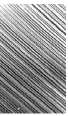
Figure 2.2: Typical layer structure.
M− is based on the direction of its shearing. This configuration results in a typical surface
texture (see Figure 2.2), often observed with specimen under tensile testing. Here, the
layers are formed of austenite and the martensite variant favorably oriented to the loading
direction. Motivated by this observation, the model considers a mesoscopic layer as the
basic element and assumes the macroscopic material as a stack of such layers.
Figure 2.3 illustrates this understanding of the mesoscopic material structure. The
single crystal is represented by the fact that all layers are aligned with the same angle to
the loading direction. In addition to the layer alignment, Figure 2.3 presents the mechanism
of the shape memory effect. At the very left, the material is in a load-free state at a low
temperature and consists of both martensite phasesM±. The orientation of one martensite
phase is favorable for tension and the other one for compression. In the second illustration
from the left, a tensile force is applied to the specimen, and the layers with the compression
orientation start to erect caused by the shear stress in the plane. Once a critical tensile force
is achieved, these layers flip in the other martensite phase (middle) and, thus, contribute to an extension in the specimen’s length. Most of this extension remains, when the load
is released from the specimen due to the fact that no reverse transformation occurs (2nd
from right). This residual deformation can be restored by heating. The specimen contracts
back to its original shape (right) due to a transformation from martensite to austenite. A
subsequent load-free cooling transforms this austenite into the twinned martensite structure
Figure 2.3: Layer model of a macroscopic material
2.2
Free Energy as Central Quantity
Depending on its shear deformation ε and temperature T, the lattice layers have a
deter-mined free energy. We consider every layer as an ensemble of lattice particles being in
the same phase. The governing potential for the thermo-mechanical behavior of such an
ensemble is the Helmholtz free energyΨ=U−T S consisting of the internal energyU and the entropyS. Figure 2.4 (left) shows a schematic sketch of a typical free energy at afixed temperature and without the action of an external load, where all three phases are stable.
It consists of a chain of parabolae; three of them are convex and two concave. The convex
parabolae belong to the three phase, whereas the two concave ones are energy barriers
sep-arating them. Figure 2.4 (right) illustrates the action of an external load σ. Its work−σε needs to be added to the free energy.
We derive the Helmholtz free energy Ψwith arguments from statistical mechanics and refer the interested reader to [70] for details. Since the free energy is a function of the
temperature, we would like to discuss its influence using Figure 2.5 for a specimen made
Figure 2.4: Free energy of a lattice layer for a fixed temperature without (left) and with external load (right).
An increase in temperature to T = 300K yields to the creation of a third minimum, which belongs to the austenite phase. Upon further heating to T = 305K the center minimum represents already a lower energy than the ones belonging to the martensite
phases, but the remaining energy barrier between the phases prevents a transformation
from happening. This occurred already atT = 328K since the austenite is the only stable phase at this temperature, and the energy barriers were eliminated. One identifies this
process as entropic stabilization of the austenite; the reversal is the formation of the
so-called temperature induced martensite.
Under the action of an external load σ the Gibbs free energy becomes the governing
thermodynamic potential for a lattice layer. We discuss the effect of an increasing load
using Figure 2.6 for a fixed temperatureT = 328K. The illustration at the top left shows the load-free state, where the Helmholtz and Gibbs free energy are identical, and, thus, is
the same plot as the last one in Figure 2.5.
An increasing load to σ = 50M P a lowers the minimum for M+ and raises the one for
M−. We observe that the austenite is still stable with the lowest energy minimum. This
changes for σ = 150M P a, where the austenite remains stable, although the martensite M+ the same energy. Since both minima are still separated by an energy well, no phase
Figure 2.6: Free energy for a lattice layer forT = 328K and different loads.
martensitic phase.
Along with this phase transformation goes a significant increase in the specimen’s strain.
Subsequent unloading of the specimen to σ= 150M P adoes not result in a phase mation, since Figure 2.6 shows a present energy barrier for this load. The reverse
transfor-mation to the martensite phase will occur at lower load, restoring the transfortransfor-mation strain
and, thus, creating a typical stress vs. strain hysteresis. We identify this as the pseudoelastic
material behavior of the shape memory typically occurring at high temperatures.
2.3
Stress-Strain Relation
The quantity of greatest interest is the resultant change in the specimen length caused by
∆ denotes its actual deformation and l its original length in loading direction. Therefore the strain of the entire specimen
ε=xAεA+x+ε++x−ε− (2.1)
is determined as the sum of the strain of each phase weighted by its fraction, where
xA, x+, x− denote the phase fractions and εA, ε+, ε− the strain of each phase. Since there are three phases in the material considered, we know that the sum of all phase fractions
needs to equal one.
1 =xA+x++x− (2.2)
Caused by thermal activation, the layers fluctuate about its energy minimum. We assume that all layers of one phase are in a thermodynamic equilibrium among each other,
and the expected value for its strain can be calculated with argument from statistical
mechanics, e.g.
εA=
Z +wA(T)
−wA(T)
εexp−G(ε, T, σ) kBT
dσ
R+wA(T)
−wA(T) exp−
G(ε,T,σ)
kBT dσ
(2.3)
In (2.3) T denotes the temperature, kB the Boltzmann constant and G(ε, T, σ) the
Gibbs free energy. The integration limits±wA(T)are the transition points with the concave
parabolae.
Since εA in (2.3) is a function of the stressσ, we call (2.1) the stress-strain relation for
the single crystal SMA, where the deformation also depends on the temperature and the
internal state of the specimen is determined by the phase fractions.
2.4
Kinetics of Phase Transformation
We determine the phase fractions by the integration of the ODE system
·
x+ = −x+p+A+xApA+ (2.4)
·
The equations in (2.4) and (2.5) are kinetic rate laws for the phase fractions and describe
their evolution in time. They are derived with arguments from the theory of thermally
activated processes. The fraction of, e.g., martensiteM+can only be altered by an exchange
of particles with its neighboring phase. Hereby, this exchange consists of a loss proportional
to the number of layers in the M+ phase and a gain, which is proportional to the number
of layers in the austenite phase. The factors of proportionality are pαβ and the phase
transformation probabilities for the transformation from phaseαto the phase β.
They are derived with arguments from statistical mechanics andp+A, e.g., can be written as
p+A=
v u u
t kBT
2πmV 2 3
L
exp³−G(σ,wm(T),T)
kBT ´
R+∞
wm(T)exp ³
−G(kσ,ε,TBT ) ´
dε
(2.6)
Equation (2.6) describes the probability of a layer of martensite M+ to surpass the
energy barrier evaluated at the location wm(T) of the energy barrier. We introduced
VL as the activation volume of a lattice element, kB the Boltzman constant, and T the
temperature of the SMA.
In order to evaluate (2.6), we need to determine G(σ, ε, T) considering its definition
G(σ, ε, T) :=Ψ(ε, T)−σε (2.7)
and a chain offive parabolae forΨ(ε, T)as shown in Figure 2.4. The following conditions and assumptions were used to determineΨ(ε, T) :
1. Smoothness for the transition points. The values and derivatives of the convex and
concave parabolae, evaluated at the transition points, must be equal. We denote the
transition points between the concave parabola and the austenite A and martensite
M± aswA,M(T) respectively.
2. We know for the stressσ=∂Ψ/∂εand, therefore, can evaluate the condition∂2Ψ/∂ε2 = ∂σ/∂εatwA,M(T) using µ
∂σ ∂ε
A,M
=EA,M (2.8)
3. The minima of the convex parabolae in the load-free case are located at zero strainε
4. For a reference temperatureTR we assume Ψ(±εT, TR) = 0 and Ψ(0, TR) =∆β(TR),
where∆β(T) is unknown at this point.
The result is a system of equations, where we can solve the equations for the convex
parabolae immediately considering EA,M as to be known. Subsequently, the equations for
the concave parabolae were solved; they remain a function of wA,M and ∆β(T), and we
have
Ψ(ε, T) = 1
2EM(ε+εT)
2 ε <
−wM
Aε2+Bε+C −wM ≤ε <−wA
1 2EAε
2+∆β(T)
−wA≤ε < wA
Aε2−Bε+C wA≤ε < wM
1
2EM(ε−εT)
2 w
M ≤ε
(2.9)
with
A = EM(εT −wM) +EAwA 2 (wA−wM)
(2.10)
B = wA[EM(εT −wM) +EAwM] wA−wM
(2.11)
C = 2∆β(T) (wA−wM) +w
2
A[EM(εT −wM) +EAwM]
2 (wA−wM)
(2.12)
Furthermore, we determine ∆β(T) as a function of wA,M from the set of equations
resulting from the conditions for Ψ(ε, T) as
∆β(T) = 1
2[EM(εT −wA) (εT −wM)−EAwAwM] (2.13) Finally, we introduce the stressesσAgoverning the austenite-martensite transformation
andσM governing its reversal. They both can be determined from two tensile experiments,
since they both depend on the temperature. It is a good assumption to assume their
temperature dependence as to be linear in the relevant temperature regime. This allows for
the determination of wA,M since we evalute σ =∂Ψ/∂ε at the transition points as shown
σA = µ ∂Ψ ∂ε ¶ wA (2.14)
σM =
µ ∂Ψ ∂ε ¶ wM (2.15)
We finally solve (2.14) and (2.15) forwA and wM:
wA =
σA
EA
(2.16)
wM =
σM
EM
+εT (2.17)
We summarize that the Gibbs free energy can be uniquely identified knowing the
mate-rial parameters σA, σM, EA, EM.
Substituting (2.9)-(2.17) in (2.7) allows for the evalution of the phase probability
trans-formations, and we get for the martensite-austenite transformation
p±A= 2 τx
r
EM
EA
1 erfcx(αMzM)
(2.18)
where
αM : =
r
VS
2EMkBT
(2.19)
zM : =σM ∓σ (2.20)
Similarily, we derive the probabilities for the reverse transformation as
pA±= 2 τx
[erfcx(−αAzA)−erfcx(2αAσA−αAzA) exp (4αAσA(αAzA−αAσA))]−1
(2.21)
where
αA : =
r
VS
2EAkBT
(2.22)
2.5
Balance of Internal Energy
Since the stress-strain relation as well as the phase fractions are also temperature-dependent,
we need to include an equation for the temperature T and assume this temperature as to
be homogeneous. This equation is derived from the balance of the internal energyU
dU dt =
·
Q+σεV,· (2.24)
and we rewrite it using the enthalphy H:=U −σεV as
dH dt =
·
Q−σεV· (2.25)
Hereby Q· is the heat input rate and σεV· the term representing the power of external
forces. We furthermore assume that the total enthalphy is the sum of the enthalpies of all
particles in one phase and have
H=X
α
(xαhα(σ, T))V (2.26)
whereV is the SMAs volume,xα denotes the volume phase fraction andhα the specific
enthalphy. We introduce (2.26) in (2.25) and consider the total differential for hα
dhα
dt = ∂hα
∂σ ·
σ+∂hα ∂T
·
T (2.27)
as well as
∂hα
∂σ = ∂g ∂σ −T
∂s ∂σ =
∂g
∂σ =−ε (2.28)
knowing that the specific entropy is independent of the stress and that g denotes the
specific Gibbs free energy.
The resulting equation for the temperature evolution in time
cT· = · Q V −
·
x+(h+−hA)−x·−(h−−hA) (2.29)
considers c = ∂hα
∂T , the specific heat of the SMA and hα the specific enthalphy of the
phases M+, M− and A respectively. The relevant heat supply terms for the SMA are
electric current. Considering this and rearranging (2.29) leads the final form of the energy balance
ρcVT· =−hAs(T −T0) +j(t)−x·+H+V −x·−H−V (2.30) This is a third ordinary differential equation (ODE) that needs to be solved
simultane-ously with the rate laws (2.4) and (2.5) for the phase fractions. Since the ODE system is
characterized by an extreme numerical stiffness, which is also varying with its non-linearity,
we use the Radau5 method for its integration. The method is described in [33] and considers
a 5th order Runge-Kutta scheme with step size control.
In (2.30) ρ denotes the density of the SMA, c its specific heat, V its Volume, h the
film coefficient, As the surface area and T0 the ambient temperature. The temperature of
a SMA can be changed by heat exchange with the environment, by Joule heatingj(t), and through the latent heats H± of the phase transformation, where we define
H± :=h±−hA (2.31)
Since hα is a specific enthalpy, we can determineH±as the difference of the Helmholtz free energy for T = 0evaluated at the associated minima.
2.6
Summary of Model Equations and Simulation of
Hys-teresis Loops
In order to simulate the material behavior of the perfect single crystal SMA, we need to
integrate the rate laws for the phase fractions (2.4) and (2.5) as well as the balance of the
internal energy (2.30) simultaneously. The solution of this ODE sytem
·
x+ = −x+p+A+xApA+ (2.32)
·
x− = −x−p−A+xApA− (2.33)
ρcVT· = −hAs(T−T0) +j(t)−x·+H+V −x·−H−V (2.34)
allows to evaluate the stress-strain relation (2.1)
Figure 2.7: Isothermal, mechanical response of a single crystal SMA for different temper-atures. Quasi-plastic (left, T = 280K), transition to pseudo-elastic (middle, T = 308K), and pseudo-elastic material behavior (right,T = 338K).
to determine the macroscopic mechanical material behavior.
Figure 2.7 exemplarily illustrates the stress-strain behavior for an isothermal, strain
con-trolled tensile experiment at different temperatures. The left picture in Figure 2.7 shows
the low temperature, the quasiplastic, material behavior. The hysteresis is located around
the origin, because there is no austenite stable atT = 280K and the phase transformations only occur between the two martensite phasesM+ and M−. With increasing temperature
the pseudoelastic material behavior develops and is fully pronounced at the highest
tem-perature T = 338K in the right picture of Figure 2.7. Phase transformations occur here between austeniteA and martensiteM±, where the stress level of the hysteresis shifts with
the temperature.
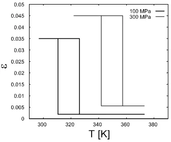
The strain vs. temperature relation shown in Figure 2.8 is typical for an experiment,
where the temperature of the SMA is cycled up and down under the action of afixed load. It is a direct consequence of the material behavior presented in Figure 2.7. Furthermore,
we observe that an increasing load shift this strain-temperature hysteresis to higher strains
and temperature levels. The diagram in 2.8 symbolizes the input-output relation for an
SMA actuator, where the output, its strain, is controlled by the temperature input.
We can summarize that the model is able to describe the temperature dependent
mate-rial behavior in the regime of quasiplasticity and pseudo elasticity. The hysteresis in both
regimes are characterized by sharp transitions and pronounced plateaus. The right picture
Figure 2.8: Strain vs. temperature behavior for two different loads.
Upon unloading we observe a reversible unloading path through the hysteresis, which is not
typically observed in experiments. The data usually shows the formation of minor hysteresis
loops embedded in the major, outer hystersis.
Since, the model is based on the assumption of a perfectly homogeneous material, its
behavior is not typical and realistic. Therefore, in the next chapter we will focus on an
Inhomogeneous Polycrystal Model - Direct
Implementation
The previous chapter described the basic structure of a model for single crystalline behavior
under the assumption of a perfectly homogeneous material. In regard to commercially
available SMA material, neither of the two is correct; and if we want to model the behavior
of "real life" engineering components like, e.g., stents, actuator wires or thinfilm devices in MEMS applications, we need to extend the above model. This section will develop a version,
which accounts for inhomogeneities and interaction between different phases and grains as
encountered in a typical polycrystalline material. After the introduction of the concept with
a focus on the two commonly encountered loading types, stress control and strain control,
we perform a convergence analysis for the isothermal and non-isothermal case. Finally, we
discuss the effects of different model parameters on the resulting hysteresis loops.
3.1
Concept of Stochastic Homogenization
The homogeneity assumptions made for the derivation of the perfect single crystal model in
the previous chapter certainly hold at best for small length scales only (micro- or meso-level).
For the description of the macroscopic behavior of SMA materials, we have to account for
effects like grain boundaries, or even within a single grain, lattice faults and impurities.
These effects have an impact in particular on the energy barrier separating two phases from
one another. In contrast to the perfect single crystal, where each mesoscopic lattice particle
saw the same energy barrier, it will now be assumed that each lattice particle can
poten-tially have a barrier of its own, see Figure 3.1 (top left). Note that barriers are restricted to
unstable concave regions, which are also known as spinodal regions. The minimum barrier
is the one represented by the well known tangent construction from equilibrium
thermody-namics. Any barrier with a convex shape would actually not represent a barrier and destroy
the multi-phase character of the energy.
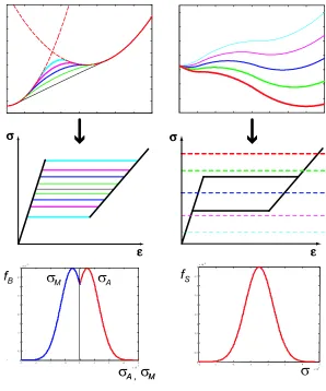
Figure 3.1: Effect of distribution in barrier (left) and internal stress (right). In addition to the aforementioned effects, inhomogeneity leads to another mechanism
that needs to be accounted for in order to describe the macroscopic behavior realistically.
transforming particles, a particular lattice particle does not necessarily see the externally
applied stress σ only, but an additional interaction stress σi superimposed to it. This
leads to the concept of an effective stress σef f = σ+σi, which drives the actual material
response. This is similar to well known concepts in magnetics, see, e.g., [10]. In addition to
different barriers, lattice particles may thus also see differently distorted energy landscapes,
which biases the resulting barriers in one direction. This effect is illustrated in Figure 3.1
(top right). The center row of Figure 3.1 shows the stress-strain diagrams resulting from
the various energies in the top row. It can be seen that different energy barriers lead to
hysteresis loops with different thicknesses. The higher the energy barrier the thicker the
hysteresis, and the minimum barrier corresponds to a zero thickness hysteresis, indicating
a reversible transformation at the so-called Maxwell stress.
As we are interested in the resulting macroscopic behavior, we do not resolve the spatial
location of each lattice particle with its corresponding combination of energy barrier and
effective stress. We rather assume a certain distribution, characterized by a probability
density function, giving the fraction of particles with a particular combination, which
actu-ally exist in the control volume. We then apply a stochastic homogenization procedure to
compute the average strain in the control volume based on
εave=
Z +∞
σM axw
Z +∞
−∞
ε(σi, σA)fi(σi)fA(σA)dσidσA (3.1)
In Eq. (3.1),
ε(σi, σA) =
σ+σi
EM
·
x+(σi, σA) +x−(σi, σA) +
EM
EA
xA(σi, σA)
¸
(3.2)
+ [xA(σi, σA)−x−(σi, σA)]εT
denotes the strain contribution of a lattice particle with energy barrier and interaction stress
σA, σi,respectively, andfi(σi)andfA(σA)are the probabilities to encounter a particle with
these values. The distribution in energy barriers is best formulated in terms of the barrier
stresses σA and σM, representing the upper and lower plateau stresses of the hysteresis
loops in the center row of Figure 3.1. Because of the definition σ :=∂ψ/∂ε, these stresses are identified as the slopes of the Helmholtz free energy functionψat the connection points
the Maxwell stressσMaxw,respectively, and their distributions are shown as clipped normal
distributions together with the normal distribution inσi in the bottom row of Figure 3.1.
3.1.1
Stress vs. Strain Control
A similar version of this model has already been presented in [58] and [59] for the case
of stress control using Equation (3.1). Typically however, experiments with SMAs are
conducted in strain control mode, in particular when the rate-dependent behavior is studied.
For this purpose we have to invert (3.1) such that the stress can be computed in response
to prescribed strain. Substitution ofε(σi, σA) in (3.1) using (3.2) results in
εave =σI1+I2+I3 (3.3)
where
I1 =
Z +∞
σM axw
Z +∞
−∞ 1 EM
·
x+(σi, σA) +x−(σi, σA) +
EM
EA
xA(σi, σA)
¸
(3.4)
×fi(σi)fA(σA)dσidσA
I2 =
Z +∞
σM axw
Z +∞
−∞ σi
EM
·
x+(σi, σA) +x−(σi, σA) +
EM
EA
xA(σi, σA)
¸
(3.5)
×fi(σi)fA(σA)dσidσA
I3 =
Z +∞
σM axw
Z +∞
−∞
εT[xA(σi, σA)−x−(σi, σA)] (3.6)
×fi(σi)fA(σA)dσidσA .
Inverting Eq. (3.3) and using (3.4) - (3.6), we can now easily determine the external
stress in the SMAσ as
σ = ε−I2−I3 I1
. (3.7)
All of the integrals can be solved numerically using a Gaussian quadrature method, e.g.,
εave= NA X m=1 Ni X n=1
wnmε(σi,n, σA,m)fi(σi,n)fA(σA,m) (3.8)
for Eq. (3.1).
When the strain is prescribed as a function of time, we proceed to solve for the stress
1. Choose a suitable number of integration points. The Gauss method automatically
determines the abscissae pointsσi,n,andσA,m and the corresponding weightswnm.
2. For given initial valuesx±(0),wefirst compute the integralsI1−I3 from (3.4) - (3.6).
then
3. Determine the stress σ from (3.7).
4. Solve the system (2.4), (2.5), (2.30) for each single crystal with σef f =σ+σi,n, and
σA,m to compute new phase fractions at time t1.
5. Compute the new stress again from (3.7).
6. Repeat steps 2 - 5 until thefinal time is reached.
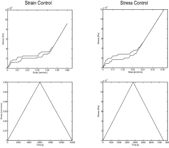
In Figure 3.4 we show results for both loading types for a very small number of
inte-gration points (3×3). It is clear that this number is not sufficient to represent smooth hysteresis curves, but it allows us to illustrate the underlying mechanisms and to highlight
the differences between the two loading types. Instead of the normal distribution shown in
Figure 3.1, we use the Laplace distribution, which for a number of observed hysteresis loops
gives a better description of the hysteresis shape. The Laplace distribution is defined as
fi(σi) =
1 2bi
exp
µ
−|σi−µi|
bi
, (3.9)
where µi denotes its mean value and bi its variance. In the above case of interaction
stress, we typically assume µi = 0, since positive and negative interaction stresses should be equally probable. For the barrier stresses, we assume
fA(σA) =
1 2bA
exp
µ
−|σAb−µA|
A
, (3.10)
with non-zero mean value µA.Note that this distribution is again clipped to begin at the Maxwell stress. The top row of Figure 3.4 shows the isothermal pseudoelastic behavior
resulting from a piecewise linear loading input ε(t) and σ(t), respectively (bottom row). The jagged behavior is the result of single crystals with corresponding effective barrier
transforming from austenite to martensite as the load increases. The width of the steps is
results in only a small increase in strain when they transform, and a larger number causes a
larger increase in strain. In both cases, the probability distribution has a rather pronounced
maximum at about the stress value, where the plateau is largest.
Figure 3.2: Comparison of strain and stress control for 9 integration points. In comparison, both cases show a similar but not identical hysteresis loop, in fact, the
strain-controlled case predicts a somewhat thinner loop and a larger transformation strain.
Inspection of Figure 3.2, which shows the time evolution of the phase fractions of each of
the 9 lattice particles involved, reveals that the kinetics of the two processes differ as well.
The stress-controlled case is characterized by instantaneous complete transformations, once
it is triggered by the external stress reaching a suitable value, while the strain-controlled
case shows a linearly increasing phase fractions, of which the slope depends on the number
a perfect single crystal with a box-shaped hysteresis loop as shown in Chapter 2, Figure 2.8
becomes unstable as soon as the stress level corresponding to the transformation plateau is
exceeded, while under strain-control it can be stabilized at each point along the plateau.
3.1.2
Convergence Analysis
Of course, the above plots do not give a reliable presentation of the stress-strain loop due to
the small number of integration points. It cannot be expected that the Gauss quadrature
has already converged for only (3×3) points, and in Figure 3.4, we study the evolution of the hysteresis loop as we increase the number of these integration points. The center
and the bottom row show the two distribution functions from Eqns. (4.14) and (4.13)
and the location of the Gauss points for a (3×3),(9×9),and (25×17)case. Comparing the first two cases, we find that the result of the "underintegration" had not only led to a non-smooth hysteresis shape, but also to a considerable underestimation of the total
transformation strain. The increase to(25×17)improves the smoothness of the hysteresis curve only, and we can consider this case to have sufficiently converged. If we inspect the
computation times shown in the header of the top row above each subfigure, however, we
see that this comes at a tremendous price. The increase in computation time from case 1
to case 2 is 226-fold, and from case 2 to case 3 is another 115 times. While the(3×3)case can be solved in 2.5 s,the total computation time for the most accurate case is thus more
than 18 hours on a typical 1 GHz PC.
The above case was solved for isothermal behavior. Subsequently, we study the
non-isothermal behavior caused by the rate-dependent release and absorption of latent heats.
For this purpose, we have to take the balance of internal energy into account as already
done for the single crystal case, see Eq. (2.30). We again assume heat conduction to
be very efficient within the material such that we can assume the temperature still to be
homogeneous, even though the latent heats are now being released and absorbed in an
in-homogeneous manner. If we average the energy balance (2.30) in the same way as we did
the strain in (3.1), we obtain:
ρcVT· =−hAs(T−T0) +j(t)− D·
x+(σi, σA)H+(σi)
E
V−
D·
x−(σi, σA)H−(σi)
E
Figure 3.4: Convergence behavior for isothermal tensile experiment. where
D·
x±(σi, σA)H±(σi)
E
=
Z +∞
σM axw
Z +∞
−∞
h·
x±(σi, σA)H±(σi)
i
(3.12)
×fi(σi)fA(σA)dσidσA
≈
NA X
m=1
Ni X
n=1
wnm
h·
x±(σi,n, σA,m)H±(σi,n)
i
(3.13)
×fi(σi,n)fA(σA,m)
It appeared from Figure 3.4 that the large number of Gauss points had provided a
at constant temperature, Figure 3.5 shows that this is not the case when we look at the
non-isothermal case. Even for (25×17) Gauss points, the temperature still exhibits a jagged behavior, see Figure 3.5 (center row). The reason can be identified from the bottom row of
the figure, which shows the production term due to the latent heats (3.13). Even though the mechanical aspects of the step-wise transformation have been smoothed out, the release
of latent heats is still discontinuous and leads to oscillations in the temperature. We did
not increase the number of Gauss points further to remove this behavior, however, as the
computation time was already unacceptably high.
3.1.3
E
ff
ects of Distribution Parameters
Instead, in the final part of this chapter, we concentrate on the effect of the distribution parameters on the hysteresis shape. Figure 3.6, shows the variation of the hysteresis, when
we change the variance parametersbiandbA.The former increases along the axis denoted by
fs,while the latter increases along thefb-axis, essentially broadening the distributions. The
upper lefthand plot closely represents the single crystal case with very narrow distributions
about the means, and we see that the effect of broadening the range of the barrier stress
σA is to tilt the plateau and distort the outer hysteresis loop. However, we can also see
that it has an impact on paths in the interior of the hysteresis. It seems as if the inner
unloading paths are lifted against the outer one, and if we look carefully we realize that,
upon unloading, the material initially moves into the hysteresis on a reversible path as in
the single crystal case. No transformation takes place on this part until the Maxwell stress
is reached. This is to be expected as the particles corresponding to the Maxwell stress are
the ones with the lowest (no) energy barrier, and should be the ones to jump backfirst. Looking down the first row of the matrix, we can see that as the distribution in inter-action stress also tilts the outer loop, it does not have an impact on the inner hysteresis
behavior. As a wider range in these stresses helps to trigger the onset of the transformation
at a lower external stress level, there is no restriction to the Maxwell stress for this
distri-bution. In fact we see that by a suitable superposition of these parameters, we can realize
a considerable spectrum of inner hysteresis paths.
Figure 3.7 focuses on inner loops resulting from partial unloading and reloading, and we
Figure 3.7: Pseudoelastic material behavior due to different distribution combinations, 2nd order loops
choices of the parameters is actually very close to what is observed experimentally.
However, as was already pointed out in the foregoing, the associated computation times
are extremely high. In particular if one were to think about potential implementations
into finite element or optimal control codes, they become prohibitive despite the good description of the material behavior. It will be the subject of the subsequent chapter to
develop a method, which preserves the positive aspects of the model, while considerably
Parameterization Method - Representative Single
Crystal
The motivation for this chapter is to present a SMA model that combines the capabilities of
the version introduced in the preceding chapter with high computational efficiency. This is
necessary for a potential implementation into other numerical codes, such asfinite element or optimal control programs or a Matlab/Simulink environment. For this purpose we will
introduce a parameterization method leading to the concept of a representative single crystal
and illustrate it for the simple case of only one distribution in eitherσAorσi.Subsequently,
we will derive the method for the more complex case of the two combined distributions from
the previous chapter and show its equivalence with the model presented therein. Finally, we
show that the method does not even need the determination of distributions, rather, based
on direct experimental determination of the barriers, it can reproduce the experimentally
observed behavior very accurately over a large range of strain rates including the minor
loop behavior.
4.1
Concept of Parameterization
The major factor hampering the performance of the Gauss Quadrature method from the
previous chapter is the necessity to solveN ×M single crystal ODE systems, withN and
M representing the number of integration points for the two distributions in barrier stress
σAand interaction stressσi, respectively. This is based on the idea of an ensemble of single
crystals with independent combinations of these two quantities, and in order to make the
evaluation of the problem more efficient, we are going to re-interpret the phase
transfor-mation process. Instead of considering the N ×M physical single crystals, we will now focus our attention on the one that is always the next in sequence to undergo the
transi-tion to the other phase. We will thus follow arepresentativesingle crystal, which means we actually switch focus from one physical crystal to the one with the next higher barrier
once it has transformed. As a consequence, this representative element sees a barrier which
changes during the process as the physical elements undergo transformations. The barrier
will increase during the loading part of the process and decrease during unloading. With
this process we have effectively parameterized the transformation by the phase fraction; and
the major advantage is that we only need to solve one ODE system as in the single crystal
case rather thanN ×M as in the previous chapter. The only formal difference is that the
barrier stress entering the transition probabilities, see Eq. (2.18,2.21) has now become a
function of the phase fraction σA(x),and this chapter will be devoted to the discussion of
the consequences of this difference.
4.1.1
Parametrization Method for a Single Distribution
We will start with the case of a single distribution in order to better illustrate the method.
Figure 4.1 shows three exemplary lattice elements with different energy barriers and thus
different barrier stresses σA for the pseudoelastic case. Here, austenite is the stable phase
and has the lowest minimum. The element at the bottom of each set represents the Maxwell
case with zero additional energy barrier, while the center and top elements have increasingly
higher barriers. During a loading process, the elements are initially all in the austenitic
phase. An applied positive stress lowers the energy barrier to the neighboring martensite
phase and favors the corresponding minimum. At a load level represented by external stress
σ2(coinciding with the Maxwell stressσM axw), the element with the lowest barrier performs
the transition to martensiteM+.Atσ3, the second one follows, and atσ4, all three elements
have transformed to M+. Unloading back to σ3, all of them remain martensitic, because
the barrier for the reverse jump back to austenite is still present (indicating a hysteresis).
Upon further unloading they consecutively transform back in the same order with the lowest