ABSTRACT
STRICKLAND, LAWRENCE ANDERSON. Computer Simulation of the Formation of Mechanically-Assembled Monolayers and Heteropolymers with Adjustable Monomer Sequences. (Under the direction of Carol K. Hall and Jan Genzer).
This thesis describes a computational investigation, using discontinuous molecular dynamics simulation, of the formation and properties of two types of self assembled polymer structures: mechanically-assembled monolayers (MAMs) and heteropolymers with adjustable monomer sequences (HAMs). MAMs are described in part 1 and HAMS are described in part 2.
MAMs in good solvent were created by grafting polymers composed of 5 to 100 hard-sphere monomers to surfaces at low density and then compressing the surface laterally at varying rates. Data for brush thickness and end-monomer density were collected as a function of surface density; this data corresponded well with theoretical predictions and simulation results performed by others. Brush thickness for all chain lengths could be controlled by judicious choice of the compression rate. Defects in the brush layer depended on chain length; we showed that quick compression for short chains allowed the layer no time to relax into coil form. Quick compression for long chains increased entanglement and allowed the chains no time to form a fully-relaxed brush. After compressing the systems to high surface densities, the brushes were relaxed to a lower surface density. It was shown that higher compression/relaxation rates led to an increase in disparity between the brush
thicknesses found during the compression and relaxation stages; this disparity was largely due to inadequate equilibration time. Last, compressing non-uniformly in the x- and y-directions showed negligible effects on monolayer height and structure.
relaxation/compression rate, we could modify the effects of brush thickness hysteresis. Finally, we suggested a general blueprint for efficient formation of defect-free monolayers.
We investigated the formation of heteropolymers with adjustable monomer sequences (HAMs) by simulating a “coloring” reaction performed on A-type homopolymers of length ranging from 100 to 300 units. The transformation of selected A-type monomers to B-type monomers along the macromolecule led to A1-x-co-Bx random copolymers, where x is the mole fraction of B. We showed that for a fixed A-B interaction, the distribution of A and B units in A1-x-co-Bx could be tuned by adjusting both the degree of “coloring” and the
solubility of the A and B segments with respect to the implicit solvent. In general, increasing the solubility of the A-type homopolymer or the degree of coloring led to a decrease in blockiness in the co-monomer distribution. Decreasing the solubility of the B species increased the blockiness of the final A1-xBx copolymer.
Computer Simulation of the Formation of Mechanically-Assembled Monolayers and Heteropolymers with Adjustable Monomer Sequences
by
Lawrence Anderson Strickland
A dissertation submitted to the Graduate Faculty of North Carolina State University
in partial fulfillment of the requirements for the degree of
Doctor of Philosophy
Chemical Engineering
Raleigh, North Carolina August 12th, 2009
APPROVED BY:
_______________________________ ______________________________
Carol K. Hall Jan Genzer
Committee Chair
________________________________ ______________________________
Keith Gubbins Orlin Velev
ii
DEDICATION
To my grandmother, Nadine S. Banks (1934-2009) . . .
who surrounded me with books and never let me go for want.
To my grandfather, Robert R. Banks . . .
iii
BIOGRAPHY
iv
ACKNOWLEDGEMENTS
I would like to take the opportunity to thank all the people whose help and support made this thesis possible.
First and foremost, I would like to thank my co-advisors, Carol K. Hall and Jan Genzer. In some ways they have been like book ends for my research, each bringing their unique strengths and expertise to bear on my research, keeping my work upright. I thank them both for taking a chance on me, allowing me to mature into a more knowledgeable researcher and scientist under their watch. I know with certainty that my time at North Carolina State University ends with me a better person professionally than the student that entered this university six years ago; for that, I am indebted. I would also like to thank Lisa Bullard for her tireless discussions and instruction about teaching and educational philosophy. She has acted both as a friend and mentor and has been a shoulder to lean on during my time at N.C. State.
I am grateful to my fellow researchers in the Hall Group who have certainly assisted in this research. Amit Goyal provided much help and discussion of my work, providing me with a sounding board to discuss the difficulties I encountered in my research. Ravish Malik also assisted with the fundamental concepts of the second part of my research. I have enjoyed my hours with the rest of the group which has always treated me more as family than coworker and provided an open door for my wife and children: Victoria Wagoner, Erin Phelps, Johnny Maury-Evertsz, Emily Boehler, Jeff Woodhead, Arthi Jayaraman and the others that have preceded us. I thank all of you for making my stay here pleasant as well as informative.
v
and Robert R. Banks, words cannot express how much I owe you. In some sense, you have created the researcher that I am today, instilling early on (nearly thirty years ago!) a love of computers and programming and fueling my constant desire to read and learn. My academic success is dedicated to the both of you; these achievements are as much yours as they are mine.
vi
TABLE OF CONTENTS
LIST OF TABLES ... viii
LIST OF FIGURES ... ix
CHAPTER 1 INTRODUCTION ... 1
1.1. ON THE COMPUTER SIMULATION OF POLYMERS ... 1
1.2. OVERVIEW ... 4
1.3. REFERENCES ... 8
CHAPTER 2 SIMULATION OF MECHANICALLY-ASSISTED MONOLAYERS IN GOOD SOLVENT ... 11
2.1. INTRODUCTION ... 11
2.2. MODEL AND METHOD ... 15
2.3. RESULTS ... 21
2.4. COMPARISON WITH SCF THEORY AND PREVIOUS RESULTS ... 27
2.5. CONCLUSIONS ... 30
2.6. REFERENCES ... 32
2.7. FIGURES ... 35
CHAPTER 3 EFFECT OF POOR SOLVENT ON MECHANICALLY- ASSISTED MONOLAYERS ... 48
3.1. INTRODUCTION ... 48
3.2. MODEL AND METHOD ... 51
3.3. RESULTS ... 55
3.4. CONCLUSIONS ... 66
3.5. REFERENCES ... 68
3.6. FIGURES ... 71
CHAPTER 4 SIMULATION OF HETEROPOLYMERS WITH ADJUSTABLE MONOMER SEQUENCES ... 86
4.1. INTRODUCTION ... 86
4.2. MOLECULAR MODEL AND SIMULATION METHOD ... 90
4.3. RESULTS AND DISCUSSION ... 94
4.4. CONCLUSION ... 105
4.5. REFERENCES ... 107
vii
CHAPTER 5 EFFECT OF TETHERING ON MONOMER SEQUENCE IN HAMS ... 120
5.1. INTRODUCTION ... 120
5.2. MOLECULAR MODEL AND SIMULATION METHOD ... 125
5.3. RESULTS AND DISCUSSION ... 128
5.4. CONCLUSION ... 137
5.5. REFERENCES ... 140
5.6. FIGURES ... 143
CHAPTER 6 FUTURE WORK ... 158
6.1. SIMULATION OF MORE ADVANCED MAMS ... 158
6.2. SIMULATE WETTING PROCESS ... 159
6.3. INVESTIGATE EFFECT OF A-B INTERACTION (HAMS) ... 160
6.4. INVESTIGATE DIFFERENT TETHERING SURFACES ... 160
6.5. FIGURES ... 162
APPENDICES ... 166
viii
LIST OF TABLES
Table 2.1 Mean-Squared z-directional Radius of Gyration, <Rg,z>2, and Radius of Gyration, <Rg>2, for M chains of N length at surface density, a. ... 20
Table 2.2 Maximum brush height, hmax, fit variables, C1 and C2, and average brush height, <z>, for chains of length, N, and surface density, a. Also shown for comparison is Murat and Grest (M&G) data. ... 28
ix
LIST OF FIGURES
Figure 2.1: (a) A system consisting of 50 polymers of 50 monomers each at an initial surface density of 0.01monomers per area is compressed every 500th collision to (b) surface density 0.200, and, (c) finally to 0.500. ... 35
Figure 2.2: Monomer density profile, (z), as a function of distance from the surface, z, for a system of fifty 50mers compressed from initial surface density a = 0.01 to final surface density a = 0.03. ... 36
Figure 2.3: Monomer density profile, (z), as a function of distance from the surface, z. The system from Figure 2 has been further compressed to (a) a = 0.10, (b) a = 0.20 and finally to (c) a = 0.50. Inset magnifies region near surface. ... 37
Figure 2.4: Orientation order parameter <cos n> as a function of monomer number along the chain, n, for surface densities a = 0.01, a = 0.03, a = 0.10, a = 0.20, and a = 0.50. ... 38
Figure 2.5: End-monomer density profile, E(z), as a function of distance from the surface, z, at surface densities a = 0.01, 0.03, 0.10, 0.20, and 0.50. Each graph has been shifted vertically 0.08 relative to the preceding graph for clarity. ... 39
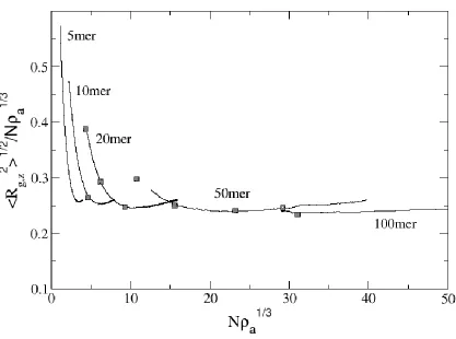
Figure 2.6: Normalized radius of gyration in the z-direction as a function of Na1/3 for 5mers, 10mers, 20mers, 50mers, and 100mers. Also shown is the equilibrium data (■) from Murat and Grest data [37]. ... 40
Figure 2.7: Ratio of the radius of gyration in the z-direction to the overall radius of gyration for 5mers, 10mers, 20mers, 50mers and 100mers as a function of surface density. ... 41
x
Figure 2.9: Mean-square radius of gyration in the z-direction as a function of surface density for a system of 50mers compressed at rates of 500, 7500 and 10,000 collisions per compression attempt. Also shown is equilibrium data from Murat and Grest [37].... 43 Figure 2.10: Plot of hysteresis in <Rg,z2> versus surface density for compression rates 100, 500 and 5000 collisions per compression attempt. Compression values are shown as symbols and relaxation values are plotted as lines. ... 44
Figure 2.11: Density profile (z) versus z showing C1/C2 fit of Equation 2.19 for 20mers at various values of a. ... 45
Figure 2.12: Density profile (z) versus z showing C1/C2 fit of Equation 2.19 for 50mers at various values of a. ... 46
Figure 2.13: Density profile (z) versus z showing C1/C2 fit of Equation 2.19 for 100mers at various values of a. ... 47
Figure 3.1: Comparison of monolayer snapshots for systems containing: (a) hard chain 50mers and (b) square-well chain 50mers at T* = 1.2 which corresponds to poor-solvent conditions. ... 71
Figure 3.2: Mean-squared radius of gyration in the z-direction, <Rg,z2>, as a function of surface density, a, for (a) twenty 20mers, (b) fifty 50mers and (c) twenty-five 100mers at various reduced temperatures, T*. Compressions were attempted once per 2000 monomer collisions. ... 72
Figure 3.3: Mean-squared radius of gyration in the z-direction, <Rg,z2>, as a function of surface density, a, for (a) twenty 20mers, (b) fifty 50mers and (c) twenty-five 100mers at various compression rates and T* = 1.2. By comparison, results from fifty 50mers (---) at 1 compression attempt per 10,000 collisions are included in (c). ... 73
Figure 3.4: Top-down view of twenty-five 100mers at T* = 1.2 at a surface density less than the critical surface density (left, a = 0.06) and greater than critical surface density (right, a = 0.065). Compressions were attempted once per 10,000 monomer collisions. 74
xi
Figure 3.6: Mean-squared radius of gyration hysteresis data for fifty 50mers at T* = 1.2 compressed/decompressed at two different rates. ... 76
Figure 3.7: Mean-squared radius of gyration hysteresis data for twenty 20mers compressed/decompressed at various reduced temperatures, T*. Compressions were attempted once per 2000 monomer collisions. ... 77
Figure 3.8: Mean-squared radius of gyration hysteresis data for twenty-five 100mers compressed/decompressed at various reduced temperatures, T*. Compressions were attempted once per 2000 monomer collisions. ... 78
Figure 3.9: End-monomer density profile for fifty 50mers compressed to surface density a = 1.0 at T* = 1.2 and various compression rates averaged over three runs. Picture on the left depicts a side view of monolayer formed during slow compression. ... 79
Figure 3.10: End-monomer density profile for twenty-five 100mers compressed to surface density a ≈ 0.85 at T* = 1.2 and various compression rates averaged over three runs. ... 80
Figure 3.11: Number of attempts per successful compression at T* = 1.2 for (a) twenty 20mers and (b) fifty 50mers as a function of surface density at various compression rates. ... 81
Figure 3.12: Number of attempts per successful compression at T* = 1.2 for twenty-five 100mers as a function of surface density at various compression rates. Picture on the left depicts trapped chains near the tethering surface for fastest compression case. ... 82
Figure 3.13: Change in surface density per change in reduced time (da/dt*) for twenty 20mers as a function of reduced time at T* = 1.2 and various compression rates. ... 83
Figure 3.14: Change in surface density per change in reduced time (da/dt*) for fifty 50mers as a function of reduced time at T* = 1.2 and various compression rates. ... 84
xii
Figure 4.1: Mean-square radius of gyration of a 300-mer containing monomers of type A as a function of kT/|AA|. The line is meant to guide the eye. The insets denote the conformations of the low-temperature globule (kT/|AA| = 0.2) and high-temperature coil (kT/|AA| = 8.0). ... 110
Figure 4.2: Mean-square radius of gyration as a function of the degree of coloring (i.e., the mole fraction of B units, x, in A1-xBx) for polymers of chain length ranging from 100 to 300 at RBA (=|BB|/|AA|) = 10.0 and kT/|AA| = 0.2 (poor solvent). ... 111
Figure 4.3: Mean-square radius of gyration, <Rg2>, as a function of the degree of coloring, x (i.e., the mole fraction of B units, x, in A1-xBx) for 300-mers at RBA (=|BB|/|AA|) = 0.5 (closed symbols) and 10 (open symbols) and various reduced temperatures (kT/|AA|) equal to a) 0.2, b) 1.6, c) 3.0 and d) 8.0. The error bars were obtained by averaging over 3 simulation runs. ... 112
Figure 4.4: Conformation of a 300-mer A1-xBx prepared by “coloring” a parent A 300-mer (grey balls) with the coloring species (red balls) to various degrees of coloring, x, ranging from 0 to 0.5 at kT/|AA| = 0.2 and RBA=|BB|/|AA| = 0.5, 1.0, 5.0 and 10.0. ... 113
Figure 4.5: (Top) Snapshot of the conformation of a A0.5B0.5 300-mer at kT/|AA| = 8.0 and RBA (=|BB|/|AA|) = 0.50. The A and B units in the copolymer are depicted by grey and red balls, respectively. (Bottom) Corresponding barcode plot for the same 300-mer. ... 114
Figure 4.6: Barcode plots for A0.5B0.5 300-mers at RBA (=|BB|/|AA|) = 5.0 and kT/|AA| equal to: a) 0.2, b) 0.6, c) 0.8, and d) 1.2. ... 115
Figure 4.7: Dispersion plot for a 300-mer A0.5B0.5 at kT/|AA| = 0.2 and RBA (=|BB|/|AA|) = 5.0. The inset depicts a log(D)-log() plot for the first 100 monomers of the chain. ... 116
xiii
Figure 4.9: Conformations of A1-xBx 300-mers at kT/|AA| = 4.0 and RBA (=|BB|/|AA|) = 5.0 at various degrees of coloring, x, ranging from 0 to 0.5. The A and B units in the copolymer are depicted by grey and red balls, respectively. ... 118
Figure 4.10: Dispersion as a function of the window size, , and degree of coloring, x, for A1-xBx 300-mers at a) kT/|AA| = 0.2 and b) kT/|AA| = 1.2. Shown as 3-D plot and contour plot. ... 119 Figure 5.1: (left) Average blockiness, defined as the slope of log(D) vs. log() [see text for explanation] as a function of the percent of coloring in diblock copolymers () and random copolymers with kT/|AA| = 0.2 [RBA = 0.5 () and RBA = 10.0 ()] and kT/|AA| = 8.0 [RBA = 0.5 () and RBA = 10.0 ()]. (right) Examples of “bar code” plots for random copolymer systems (A)-(D) marked in the left figure. For each system, the top and bottom bar codes correspond to 15 and 60% of coloring, respectively. ... 143
Figure 5.2: Snapshots of conformation of homopolymers on flat solid substrates (from top to bottom: 50-, 100- and 300-mers) at kT/|AA| = 8.0 with surface grafting densities = 0.001 (left panel) and 0.010 (right panel) polymers/area. ... 144
Figure 5.3: Snapshots of conformation of homopolymers on flat solid substrates (from top to bottom: 50-, 100- and 300-mers) at kT/|AA| = 0.2 with surface grafting densities of = 0.001 (left panel) and 0.010 (right panel) polymers/area. ... 145
Figure 5.4: Reduced grafting density of 50-mers (), 100-mers (), and 300-mers () as a function of the reduced temperature (kT/|AA|) at surface grafting densities of = 0.001 (a) and 0.010 (b) polymers/area... 146
Figure 5.5: Blockiness versus reduced temperature (kT/|AA|) for A0.5B0.5 50-mers at surface grrafting densities = 0.001 and 0.010 polymers/area and varying RBA. ... 147
Figure 5.6: Blockiness versus reduced temperature (kT/|AA|) for A0.5B0.5 100-mers at surface densities = 0.001 and 0.010 polymers/area and varying RBA. ... 148
xiv
Figure 5.8: Conformations of sixteen A0.5B0.5 300-mers (A = grey, B = red) tethered at surface densities = 0.001 and 0.010 polymers/area for kT/|AA| = 1.0 and RBA = 5.0. A snapshot of a typical bulk conformation of a corresponding bulk chain is also shown.. 150
Figure 5.9: Probability distribution for A0.5B0.5 300-mers tethered at surface densities = 0.001 and 0.010 polymers/area for kT/|AA| = 1.0 and RBA = 5.0. The inset data denote the end-monomer probability distribution... 151
Figure 5.10: Sixteen A0.5B0.5 300-mers (A = grey, B = red) tethered at = 0.010 polymers/area for kT/|AA| = 6.0 and RBA = 5.0. ... 152 Figure 5.11: Probability distribution for A0.5B0.5 300-mers tethered at surface densities = 0.001 and 0.010 polymers/area for kT/|AA| = 6.0 and RBA = 5.0. The inset data denote the end-monomer probability distribution... 153
Figure 5.12: Position along A0.5B0.5 300-mers as a function of monomer type (B = -1, A = +1) tethered at surface densities = 0.001 (left panel) and 0.010 (right panel) polymers/area for kT/|AA| = 6.0 and RBA = 5.0. Typical chain conformations are shown for each case in the upper part (A = grey, B = red). ... 154
Figure 5.13: Average blockiness at = 0.010 polymers/area plotted against the average blockiness at = 0.001 polymers/area for A0.5B0.5 of various chain lengths and kT/|AA| (ranging from 0.2 to 8, represented by the increasing size of the symbols) for RBA equal to 0.5 (a), 1.0 (b), 5.0 (c) and 10.0 (d). The dashed lines denote situations where the average blockiness is equal for both surface tethering densities. ... 155
Figure 5.14: Position along A1-xBx 300-mers at five different degrees of coloring ranging from 10 to 50% as a function of monomer type (B = -1, A = +1) tethered at surface densities = 0.001 (left panel) and 0.010 (right panel) polymers/area for kT/|AA| = 8.0 and RBA = 0.5 (top panel) and 10.0 (bottom panel). ... 156 Figure 5.15: Position along A1-xBx 300-mers at five different degrees of coloring ranging from 10 to 50% as a function of monomer type (B = -1, A = +1) tethered at surface densities = 0.001 (left panel) and 0.010 (right panel) polymers/area for kT/|AA| = 1.0 and RBA = 0.5 (top panel) and 10.0 (bottom panel). ... 157
xv
Figure 6.2: System of twenty 50mers at low grafting density (left picture) and after compression to high grafting density (right). Note the chain ordering in the right picture. ... 163
Figure 6.3: Experimental measurement of the contact angle formed by a droplet of water on the surface of a mechanically-assembled monolayer. ... 164
1
CHAPTER 1
INTRODUCTION
If we knew what we were doing, it wouldn’t be called Research. -Albert Einstein
1.1.
ON THE COMPUTER SIMULATION OF POLYMERS
Polymers are everywhere, employed in a nearly endless range of applications (as will be discussed herein): from durable plastics to silly putty, from hydrophobic monolayers to random-blocky copolymers. We are essentially surrounded by polymers in their various forms but this ubiquity does not preclude us from learning even more about them. With our hands, we are able to touch polymers, to stretch and mold them, however we are unable to understand what is happening inside at the molecular level. Meanwhile, innovation in the field of polymers depends on us digging ever deeper.
2
the short-range features found in monomeric or atomistic systems and the long-range features which arise, by definition, from the molecular weight of the polymer in question [1-4]. Other features such as side chains, backbone angles, time scales, charges and solvent qualities – all of the complexities found in nature – must be considered if one is to investigate highly complex (and ultimately, more interesting) systems [5-8]. Fortunately, the processing capability of modern computers grows increasingly more powerful each day, allowing us to advance the collective knowledge about polymers.
The focus of this study is two systems which, at first glance, seem very different: highly-dense hydrophobic monolayers and random-blocky copolymers created through a coloring process. They are, however, connected in the author’s mind by the possibility that they might in the future be combined into a single hybrid system that allows us to control the creation of copolymers with a selected blockiness. This will be discussed at the end of this chapter.
3
monomer sequences (HAMs). These heteropolymers are copolymers containing, in our case, two distinct monomer units (A and B) distributed in a disordered or random-blocky sequence throughout the chain. The interest in random-blocky copolymers (RCPs) is due to the fact that tuning the copolymer chemical composition and co-monomer sequence distribution of the A and B units profoundly affects the characteristics of the random copolymers [15-20]. We believe that by judiciously choosing the A and B chemical species, RCPs have the potential to act as polymer blend compatibilizers [21-23], adhesion promoters [24,25], and recognition agents for patterned surfaces [26-28]. Of interest then is the ability to dictate the distribution of the A and B units or, in other words, selectively choose the degree of blockiness in the resulting copolymer. This can be accomplished by simulating the method of HAMs formation first proposed by Khokhlov and others whereby one places a parent homopolymer in a simulation box, fills the box with reactant particles and allows a “coloring” reaction to proceed [29]. With few adjustments, we can simulate this process and investigate the effects of solubility, chain length and reaction time on copolymer blockiness. Additionally, we can attach these parent copolymers to a neutral, impenetrable surface and examine the effect of grafting density on the blockiness of HAMs. What we note is that through judicious choice of the system solubility and chain length and degree of coloring, one can “fine tune” the blockiness of the formed HAMs; further still, by attaching these chains to a surface at a density which allows for chain-chain interaction, one can “coarse tune” the blockiness of the formed HAMs. We see that, through computer simulation, not only can we explain the underlying physical concept at work in the formation of HAMs, we can extend that knowledge beyond the current knowledge base of experimenters.
4
the copolymers cleaved from the surface and recovered. In other words, copolymers on demand! We are reminded that research does not exist in a vacuum: what began as separate work on two distinct systems need not remain that way. This thesis lays the groundwork for such a blueprint.
1.2.
OVERVIEW
The following chapters are essentially reproductions of technical publications. Chapter 2 and 4 have been previously published, Chapter 3 is under review and Chapter 5 will be submitted for publication shortly.
5
Compressing to high surface density also results in end-monomer units located far from the tethering surface which is desired in “good” MAM formation. We note that, in general, a slow compression rate reduces discrepancies between our brush heights and values from previous simulation results collected at equilibrium. Similarly, slow compression rate reduces hysteresis effects in the monolayer.
In Chapter 3 we investigate the effect of poor solubility on the formation of mechanically-assembled monolayers. We attached chains on a surface at low grafting density as before and introduced an attractive force between non-bound monomers to replicate poor solubility conditions. Compression/relaxation rates were varied; a wide range of solvent quality was investigated. We note that poor solvent quality presents two major drawbacks for monolayers: 1) loss of surface coverage and 2) loss of monolayer order/thickness. To counter loss of surface coverage, monolayers must be compressed beyond critical coverage density; additionally, to counteract the loss of monolayer thickness, compression must occur at a rate that reduces chain entanglement. We also note the effects of poor solubility and compression rate on hysteresis, brush order and the location of end monomers (a sign of layer defects): all of which would result in a monolayer with poor barrier properties. Finally, we compared the actual compression rates in the poor solvent systems to the actual compression rates in the good solvent systems and suggested a course of action for experimenters to follow when fabricating MAMs on a large scale.
6
poor parent homopolymer solubility initially causes the copolymer to swell as B monomers move into the globule away from the solvent; on the other hand, poor B-solubility coupled with good parent homopolymer solubility led to the formation of blocky sub-globules.
In Chapter 5 we discuss the creation of HAMs when the parent homopolymer has been anchored to a neutral, impenetrable surface. In this case, we can examine the effect of the same variables as in Chapter 4 (chain length, system temperature, solubility and degree of “coloring”) but, because the polymers are tethered, we also examine the effects of grafting density coupled with varying chain length on copolymer blockiness. In general, we note that system temperature, solubility and degree of “coloring” can be used to fine tune the blockiness of the copolymer. However, variation of the surface density (as it relates to chain length) would allow researchers to adjust blockiness on a much larger scale. We note the following trends from our data. First, at surface densities below the critical coverage density, HAMs formation tethered to a surface is equivalent to HAMs formation in the bulk (Chapter 4) due to the lack of chain-chain interactions. Above the critical coverage density, an increase in surface density or an increase in chain length generally leads to an increase in blockiness in the formed copolymer. Also, we found that for an equivalent increase in surface density, longer chain lengths become relatively more blocky than shorter chain lengths. We conclude that the blockiness of random-block copolymers can be tuned for their specific end-use by optimizing the system variables discussed here: system temperature, chain length, solubility, grafting density and degree of “coloring”.
Chapter 2 was adapted from the following publication:
Chapter 2 Strickland, L. A.; Hall, C. K.; Genzer, J. “Simulation of Mechanically Assembled Monolayers and Polymers in Good Solvent Using Discontinuous Molecular Dynamics”, Macromolecules, 41, 6573 (2008).
Chapter 3 has recently been submitted to Macromolecules. Chapter 4 was adapted from the following publication:
7
8
1.3.
REFERENCES
1. M.P. Allen and D. J. Tildesley, Computer Simulation of Liquids (Clarendon Press, Oxford, 1987.)
2. K. Binder, Makromol. Chem., Macromol. Symp. 50, 1 (1991).
3. D. Y. Yoon, G. D. Smith and T. Matsuda, J. Chem Phys. 98, 10037 (1993). 4. G. D. Smith, R. L. Jaffe and D. Y. Yoon, Macromolecules, 26, 293 (1993). 5. D. Steele, J Chem. Soc. Faraday Trans. II 81, 1077 (1985)
6. J.P. Ryckaert, Physica A: Statistical and Theoretical Physics, 213, 1, 50 (1995) 7. R. Hentschke, R. G. Winkler, J. Chem. Phys, 99 5528 (1993)
8. J.J. De Pablo, M. Laso, U.W. Suter, Macromolecules, vol 26 23, 6180 (1993)
9. Adamson, A. W. In Physical Chemistry of Surfaces, 4th ed..; Wiley-Interscience: NY, 1984.
10.Kuhn, H.; Mobius, D. In Techniques of Chemistry; Wiley: NY, 1972; p 577.
11.Richard, M.A.; Deutch, J.; Whitesides, G.M. Hydrogenation Of Oriented Monolayers Of Omega-Unsaturated Fatty-Acids Supported On Platinum. J. Am. Chem. Soc. 1978, 100 (21), pp 6613-6625.
12.Waldbillig, R.C.; Robertson, J.D.; McIntosh, T.J. Images Of Divalent-Cations In Unstained Symmetric And Asymmetric Lipid Bilayers. Biochim. Phiophys. Acta 1976, 448 (1), pp 1-14.
9
14.J. Genzer, K. Efimenko Science, 290, 2130-2133 (2000). 15.Balazs, A.C.; Gempe, M. Macromolecules 1991, 24, 167-176.
16.Chai, Z.K..; Sun, R.N..; Karasz, F.E. Macromolecules 1992, 25, 6113-6118.
17.Angerman, H.; Hadziioannou, G.; ten Brinke, G. Physical Review E 1994, 50 (5), 3808-3813.
18.Smith, G.D.; Russell, T.P., Kulaserke, R.; et al. Macromolecules 1996, 29 (11), 4120-4124.
19.Simmons, E.R.; Chakraborty, A.K. Journal of Chemical Physics 1998, 109 (19), 5493-5496.
20.Bernard, B.; Brown, H.R.; Hawker, C.J.; et al. Macromolecules 1999, 32(19), 6254-6260.
21.Faldi, A.; Genzer, J.; Composto, R. J.; Dozier, W. D. Phys. Rev. Lett. 1995, 74, 3388. 22.Genzer, J.; Composto, R. J. Macromolecules 1998, 31, 870.
23.Pellegrini, N. N.; Sikka, M.; Satija, S. K.; Winey, K. I. Polymer 2000, 41 (7), 2701-2704.
24.Eastwood, E.A.; Dadmun, M.D. Macromolecules 2002, 35, 5069-5077.
25.Montanari, A.; Mueller, M.; Mezard, M. Physical Review Letters 2004, 92 (18), 185509.
10
27.Bratko, D.; Chakraborty, A.K.; Shakhnovich, E.I. Chemical Physics Letters 1997, 280, 46-52.
11
CHAPTER 2
SIMULATION OF MECHANICALLY-ASSISTED MONOLAYERS
IN GOOD SOLVENT
2.1.
INTRODUCTION
Mechanically-assembled monolayers (MAMs) are polymer brushes formed by end-grafting polymers onto a pre-stretched surface and then releasing the stretch, thereby increasing the surface density to levels higher than those typically found in systems composed solely of self-assembled monolayers (SAMs). Self-assembled monolayers are used in a variety of fields, including lubrication [1], electrochemistry [2,3], electronic and vibrational spectroscopy [4,5], photochemistry [4,6], electrical conduction [4,7], catalysis [8] and organic membranes [9,10]. Due to this wide array of uses, the ability to “tune” the surface characteristics of these monolayers is of vital importance. Although self-assembled monolayers allow for some adjustment of surface characteristics, their utility is limited due to the relatively low surface density of the grafting sites and the accompanying defects that allow penetration of liquids into the monolayer, especially polar liquids.
12
which reach higher surface coverage than those achievable solely through self-assembly, thereby impeding or retarding surface degradation from liquid penetration. To this point, all of the research in the area of mechanically-assembled monolayers has been experimental [11-13]. In pioneering work, Genzer and coworkers showed that mechanical stretching of a flexible substrate surface prior to tethering the oligomers or polymers through self-assembly would lead to the formation of dense, defect-free monolayers.
The mechanism by which chains form highly-packed MAMs is unclear. During the fabrication of MAMs, the surface strain is released, thereby increasing the surface density of the grafted molecules. As the layer shrinks, it densifies and becomes more ordered. The mechanism underlying this rearrangement process is unknown. It could be that a select polymer acts as a seed for nucleation around which other chains aggregate, generating an organized structure which then propagates throughout the entire surface. Alternatively, small localized groupings of a few molecules could form, which are then brought together mechanically as the stretch is released; organization of the entire layer would then occur on a global level. Also, the solvent quality and the rate at which the surface is released affect the thickness and ordering of the monolayer structure. Theory and previous experimental work can predict monolayer properties when the surface density is held constant. This work focuses on the densification which occurs in the MAMs formation process.
Surface-grafted polymers stretching in good solvent conditions were first studied by Alexander and de Gennes [14,15]. Based on the “blob” model [16], Alexander postulated that the monomer segment density profile for a monolayer, (h), could be expressed as
(h) = a(3-1)/2 h(1-3)(2-d)/2 (2.1)
13
height hmax, defined as the thickness of the layer over which the brush density is constant, scales as:
hmax ~ Na1/3 (2.2)
where N is the chain length of the polymer, provided that a is above the critical overlap density, *a ~ N-6/5. Below *a, hmax is nearly independent of surface density. Equation 2.2 reveals that the height of a two-dimensional monolayer (d=2) depends linearly on the length of the chain.
The work of Alexander and de Gennes was expanded upon by Skvortsov et al. [17], Milner et al. [18,19] and Zhulina et al [20]. Zhulina et al. used numerical self-consistent field (SCF) theory to show that the density profile for a monolayer of long chains in good solvent is independent of distance from the tethering surface, but that for short chains at distances near the surface, the density profile is instead parabolic. Zhulina et al. found that the density profile, (h), could be expressed as:
(h) = C1 a2/3 – C2 (h/N)2 (2.3)
where C1 and C2 are spatial-constraint constants and h is the height above the surface. Numerous simulations and experimental studies have validated the parabolic density profile model for tethered polymers[21-24]. Similarly, it was shown that the density profile for tethered polymer tail groups [E(h)] for moderate density brushes (eq. 2.4) and for more dense brushes (eq. 2.5) is given by:
14
where hmax is the maximum brush height and thickness at which the density vanishes [16, 25]. Due to the –1/2 exponential power for the more dense brush, eq 2.5 diverges at h ~ hmax, meaning most of the polymer ends are far from the wall. It should also be noted that according to equations 2.4 and 2.5, E(h) is implicitly non-zero for all h greater then zero. Thus, tail groups are not restricted to inhabiting only the outer reaches of the tethered film but are also allowed to explore space near the tethering surface.
In this paper, we present the results of discontinuous molecular dynamics simulations of the compression of systems of polymers modeled as hard chains in an attempt to mimic the MAMs formation process. Polymers of chain lengths ranging from 5 to 100 were initially grafted to a surface at low density (typically, below 0.200 monomers/area) and allowed to equilibrate. These layers were then compressed at varying rates to high surface density to study the effects of chain length and compression rate on monolayer formation. Select systems were decompressed to the initial surface density to study hysteresis effects. Finally, monolayers were compressed disproportionally in one direction to investigate the effects of non-uniform compression on ordering.
Highlights of this work are as follows. Data presented show that regardless of compression rate, monomer density profiles for the monolayer fit theoretical predictions and previous experimental work to a close approximation. We show that throughout the MAMs formation, the monolayer thickness consistently scales as Na1/3, in accordance with the theory of Alexander and DeGennes. We see that compression allows for high surface densities which would be difficult to attain solely through self assembly and that this high surface coverage and compression engenders quasi-crystalline formation near the surface and “encourages” end-monomers to move away from the surface. Last, when monolayers are allowed to relax to the original surface density or non-uniform compression is applied, the effect on layer formation is negligible.
15
compression rates and modes. In section 2.4, we compare these results with theoretical predictions and previous simulations. Section 2.5 concludes with a short summary of the results and a discussion.
2.2.
MODEL AND METHOD
We simulate the formation of a mechanically-assembled monolayer by using the discontinuous molecular dynamics (DMD) method. Traditional molecular dynamics employs a monomer-monomer interaction potential that is a continuous function of their separation (i.e. the Lennard-Jones potential), which incorporates short-range repulsions as well as long-range attractions. The trajectories of a system of monomers are repeatedly advanced at a small increment in time, after which the forces between all pairs of monomers are reevaluated. DMD, on the other hand, replaces the continuous potential function with a discontinuous function, such as a hard-sphere repulsion or square-well attraction. At long-range, monomers feel no attraction [26]. In this work, we are concerned only with short-ranged excluded volume effects. As the monomers feel only volume exclusion and no long-range attraction to one another, this implies good solvent conditions. The potential energy for non-bonded monomer-monomer interactions at distance r is given by the hardsphere potential
U(r) = ∞, r ≤ (2.6)
= 0, r >
where is the monomer diameter.
16
and the monomer’s new post-collision velocity [27,28]. The collision time between monomer i and all monomers j ≠ i is given by
(2.7)
where rij ≡ ri – rj is their relative position, vij ≡ vi – vj is their relative velocity, and bij ≡ rij ·
vij [29]. Next, the minimum collision time for the system, tc, is chosen and all monomers are
moved according to:
ri (t + tc) = ri (t) + vi (tc) (2.8)
where ri and vi represent the ith monomer’s position and velocity, respectively. At this point, exactly two monomers collide while the remainder of the monomers are separated from one another. New velocities for the colliding monomers are calculated using conservation of momentum and conservation of kinetic energy.
17
fluctuate over a range (1 ± ) [32]. In this case, the average bond lengthisand thus closer in architecture to chains constructed of tangentially-connected monomers.
The temperature of the system and, concordantly, the total kinetic energy are held constant throughout the simulation. To regulate temperature, we employ a heat bath in the form of an Andersen thermostat [33], which allows the temperature to fluctuate about an average system temperature, T*≡kBT/ . This is accomplished by having monomers collide stochastically with “ghost” particles which then change the monomers’ velocity. After particle i collides with a “ghost particle”, new collision times must be calculated for this particle and for all other particles j which, prior to the ghost collision, would have collided with i. The time between ghost collisions, tg, is random and is calculated by
tg= A · | cos(2·R) · √(-2·log(R)) | (2.9)
where R is a random number between 0 and 1 and A is a coefficient which controls the frequency with which the ghost collisions occur; A must be manipulated for each system so that the fluctuations in T are neither too big nor too small.
18
Grafting the polymers to a surface introduces an additional consideration; one must also calculate the collision time between any monomer i and the surface. For all monomers except those directly connected to the surface, this is calculated by
ti = riz / |viz| (2.10)
where riz and viz are monomer i’s position and velocity in the z-direction, respectively. (Here, the absolute value of velocity in the z-direction is required since our system is set up with the z-axis pointing away from the surface.) Also, we allow the monomer connected to the grafting surface to fluctuate over distance (1 ± ) from the hard surface. The collision time between a grafted monomer and the surface is calculated similarly to that between bonded monomers.
Periodic boundary conditions for the simulation box, which is of length Lx and width Ly, are used in the x- and y-directions. Periodic boundary conditions are not used in the z-direction since monomers are bound as chains grafted to the surface and thus, cannot escape in the z-direction. (There is no hard ceiling in the z-direction as box pressure is of no interest in this work.)
The release of previously-stretched monolayers is modeled by attempts to compress the surface at uniformally-spaced intervals. At prescribed collision numbers (say, every 500th collision), new box dimensions are calculated:
Lx (new) = Lx (old) · (1 – Lx) (2.11) Ly (new) = Ly (old) · (1 – Ly) (2.12)
19
rix (new) = rix (old) · (1 – Lx) (2.13) riy (new) = riy (old) · (1 – Ly) (2.14)
where ri is the position of monomer i. If the new positions of all particles do not violate any
excluded volume constraints or any bonded-monomer chain length constraints, the new positions are accepted. The new surface density and new surface area, a = M / (Lx,new · Ly,new) and S = Lx,new · Ly,new, respectively, are calculated. If there is a violation of constraints, the old positions and box dimensions are retained. For the purpose of this paper, the relaxation rate of the surface will be defined to be the frequency at which these compression attempts are performed; this will differ from the actual success rate of the compression.
After each compression move, data was collected for the polymer layer’s mean-square radius of gyration, <Rg2>, and the mean-square radius of gyration in the z-direction, <Rg,z2>, which are defined respectively as:
<Rg2> = 1/N · <∑(ri – rCM)2> (2.15) <Rg,z2> = 1/N · <∑(rzi – rz,CM)2> (2.16)
20
Table 2.1
Mean-Squared z-directional Radius of Gyration, <Rg,z>2, and Radius of Gyration, <Rg>2, for M chains of N length at surface density, a.
M N a <Rg,z>2 <Rg>2
50 5 0.01 0.45 1.0
50 5 0.03 0.41 1.0
50 5 0.1 0.47 1.1
50 10 0.1 1.55 3.4
50 20 0.01 2.67 7.8
50 20 0.03 3.01 7.6
50 20 0.1 5.26 8.7
50 50 0.01 10.36 24.8
50 50 0.03 13.60 25.1
50 50 0.1 29.69 38.5
50 50 0.2 49.76 55.0
25 100 0.03 55.81 81.2
21
2.3.
RESULTS
Snapshots of a system of 50 polymers composed of 50 monomers are shown in Figure 2.1 as it is compressed from (a) a = 0.01 to (b) 0.20 to (c) 0.500. We see in Figure 2.1 (b) that compression to surface density a = 0.20 overcomes one of the drawbacks of self-assembled systems: monolayer openings. Further compression to a = 0.50 thickens the monolayer and encourages movement of the polymer ends outward from the surface. These trends were followed for all systems, especially for chain lengths over N = 20.
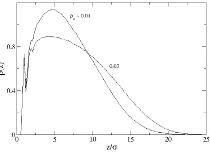
The monomer density profiles for a system of fifty 50mers at surface densities 0.01 and 0.03 are shown in Figure 2.2. We note first that the density profile at surface density a = 0.01 shows two peaks: a very sharp peak (local maximum) near 1 corresponding to the monomers from each chain directly grafted to the surface and a broader peak near 5 corresponding to the average z-coordinate values for the monomers. We note that low surface coverage encourages the chains to remain near the surface at distances 1/5th to 1/10th of their chain length, rather than to extend their conformation; we conclude that at this low surface coverage there is relatively little chain-chain interaction. Figure 2.2 also depicts the density profile for the same system compressed to surface area 0.03. While the density profile retains the sharp peak near 1 (the grafted monomers have little freedom to fluctuate), we detect an overall flattening of the profile and a general shift to the right toward higher z-values as the polymer chains straighten due to volume exclusion effects.
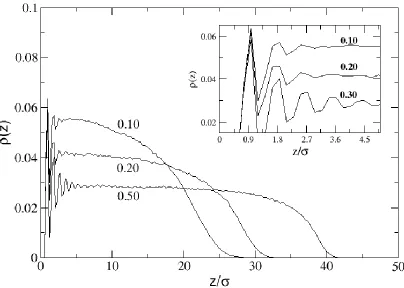
22
essentially stretching straight out from the surface. Additional evidence for this is the snapshot shown in Figure 2.1 (c). Second, the density profile oscillates near the surface. As the chains are forced to stretch out from the surface due to the high grafting density, the monomers near the surface occupy positions in the z-direction that are discrete multiples of . As can be seen in the inset of Figure 2.3, the high surface density seems to engender
order (in the z-direction) near the surface. The ordering of the layer begins at the surface and then progresses outward as the monolayer is compressed to higher surface density. However, the ordering is not truly crystalline; when viewing a top-down projection of the monomers directly attached to the surface, there is no ordering in the x- or y- direction. Thus, while there is some ordering in the z-direction due to the stretching of the chains, this is purely the result of a loss of conformational options. No ordering has propagated laterally.
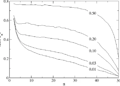
As the surface density increases due to compression, the chains align with one another. Polymer stretching and ordering is depicted in Figure 2.4 which shows the orientational order parameter, <cos n> as a function of monomer number along the chain, n, for various surface densities. Here, cos n is defined as
cos n = (zn – zn-1) / |rn – rn-1| (2.17)
23
monolayer. A chain’s ability to effectively influence the conformation of its neighbors is a direct function of its ability to stretch.
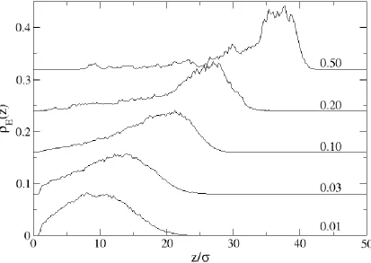
While a thick, well-organized monolayer is certainly critical in forming an impermeable brush, of equal importance is the location of the end monomers. Since end-monomer units would likely be tailored to interact with a contacting fluid, it is important that the end monomers be near the layer surface (furthest from the grafting surface). We studied how surface compression affects the location of the end-monomers. Figure 2.5 depicts the end monomer profile, E(z), for a system of 50mers. Initially, the system of chains is grafted at a surface density of a = 0.01 monomers/area. Since there is little chain-chain interaction, the end monomers are free to explore any location above z = (due to wall repulsion). Compression of the surface results in two trends: first, the end monomers naturally move away from the wall (although, E(z) is still non-zero for values z near the wall) and second, the general shape of E(z) shifts from parabolic at low densities (say, below a = 0.1) to a more sharply-defined peak at high densities (say, a = 0.50). As the surface density increases, the end monomers move from the interior of the monolayer to the outer edge.
24
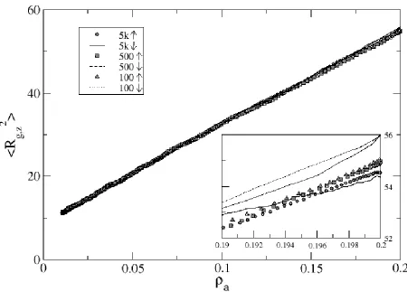
surface was compressed using a compression rate of 1 attempt per 2000 collisions. In the regime where scaling theory is applicable, <Rg,z>2 normalized by Na1/3 should be constant as a function of Na1/3 (horizontal line). On the other hand, we note that for short chain lengths (5mer and 10mer), scaling theory works only for brushes which have been compressed beyond a moderate surface density of 0.2 monomers/area (or Na1/3 ~ 3 and 6, respectively). By comparison, longer chains (50mer and 100mer) fit scaling theory for nearly all surface densities throughout compression, primarily due to their large value of N. We can infer that individual chains of the longer-chained brushes begin to interact at a lower surface density than the short-chained systems.
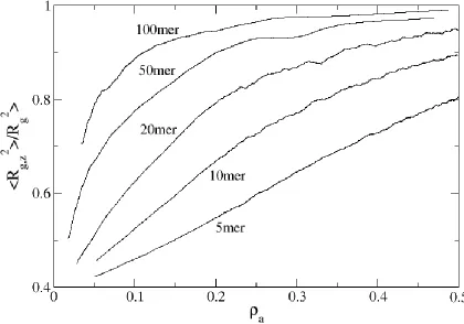
Since one advantage of using a long polymer in a brush is that it reduces the need for high surface densities, this also reduces the required amount of initial mechanical stretching of the substrate. In Figure 2.7, we plot <Rg,z>2/<Rg>2, a measure of the extension of the chains in the brush, versus surface density. Note that to develop a highly extended brush where <Rg,z>2/<Rg>2 is say 95%, one needs only a surface density of 0.2 to 0.3 monomers/area for chain lengths N ≥ 50. To reach that same proportionality though with shorter chains (e.g. N = 20), a surface area greater than 0.500 monomers/area is required; for example, 5mers would require a = 1 (idealistic and in practice wasteful). Obviously, relatively long chain lengths are in one’s best interest when producing MAMs.
25
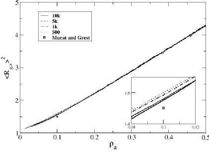
faster the surface compression, the higher the value of <Rg,z>2 (and correspondingly, the larger the difference in value from Murat and Grest’s equilibrium data). The faster compression rates do not afford the layer time to equilibrate. We can measure the relative amount of equilibration time for each system by determining the number of collisions each monomer undergoes on average between compression attempts, calculated as [shrink rate / number of chains / (chain length + 1)]. Thus, in cases of very small systems such as fifty 10mers, compression attempts every 10,000th collision allow each monomer to undergo 10,000 / 50 / 11 or approximately 18 collisions between attempt; this is significant, allowing for steady chain and brush equilibration during compression. Faster compression rates though test the layer’s ability to reorganize. The same system of fifty 10mers compressed every 500th collision averages about 0.91 collisions per monomer between collision attempts; the chains do not have a chance to relax. Therefore, experimenters must give attention to MAM formation rates, as increasing surface density too quickly leads to monolayer buckling and/or chain detachment from the surface.
While brush thickness during compression of short-chained systems tended to be higher than that of previously-published simulation results, brush thickness during compression of longer-chained systems exhibited opposite tendencies. In Figure 2.9, we show <Rg,z>2 versus surface density for 50mers. We see a similar trend as before, wherein <Rg,z>2 data for the slower rates (10k and 7.5k) are more comparable to equilibrium data than fast compression. Unlike the 10mers though, the <Rg,z>2 data for 50mers lies under the equilibrium data of Murat and Grest; most likely, the long chains are having trouble stretching through the highly-dense, thick layer to achieve the equilibrated brush height.
26
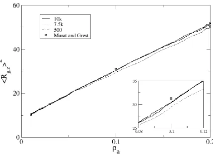
system back to the initial density by stretching the surface at the same rate as in the previous compression. This created hysteresis loops that depend on the different compression/stretch rates. Figure 2.10 shows <Rg,z>2 versus surface density for three compression/stretch rates: a compression or stretch attempt every 100th, 500th or 5,000th collision. It is noted that during the compression phase (symbols ♦,■, and ▲), <Rg,z>2-values for all three cases are roughly equal. As found earlier, varying compression rate resulted in negligible difference in monolayer thickness. The inset of Figure 2.10 depicts <Rg,z>2-values near a = 0.200 for compression (symbols) and stretch (lines) modes. The <Rg,z>2-values for the slowest stretch rate (every 5000th collisions) correspond well with the values during compression. In contrast, the <Rg,z>2-values for the fastest stretch (every 100th collision) do not match their corresponding compression data; at any value of a, brush height during stretching is 1%-2% higher than during compression.
A final area of investigation is the effect of non-uniform compression on brush formation. Experimentally, Genzer and coworkers formed MAMs by mechanically manipulating the substrate in one direction only (call it x). Thus, upon release of the stretch, grafted monomers would feel a force of compression in only the x-direction. In contrast, simulation data shown up to this point was for systems compressed equally in the x- and y-directions. To test non-uniform compression, we define a non-uniformity parameter K as:
K = (Lx,old – Lx,new) / (Ly,old – Ly,new) (2.18)
27
disparity stems from our use of periodic boundary conditions (PBCs) which mimic an infinite surface in both directions, regardless of the dimensions of the simulation box in that direction. PBCs introduce an artificial periodicity in the x- and y-directions which might cause compression effects to propagate faster than in experimental systems. Certainly we could turn off PBC to study non-uniform compression but by doing so, we lose one computational advantage at our disposal and this was not the main focus of this work.
2.4.
COMPARISON WITH SCF THEORY AND PREVIOUS RESULTS
As stated earlier, SCF theory was used to show that the density profile for polymer brushes of short chains could be described with a parabolic equation; we offer here an alternative form of equation 2.3:
(z) = 0 – z2 (2.19)
with 0 = C1a 2/3 and = C2N-2 (C1 and C2 are two adjustable parameters). Accordingly, density profile data was collected during slow compression. We plotted the normalized density profiles for 20mers, 50mers and 100mers at several densities (approximately, 0.03, 0.10, 0.20 and 0.50 monomers/area). Portions of the curves of the form A - Bz2 (equation 2.19) were fit to these profiles (Figures 2.11 through 2.13) and C1 and C2 were extracted. The goodness of the fit is primarily a function of surface density, a, and is independent of chain length: at low surface density, a, parabolic form was applicable to a majority of the chain monomers; conversely, at high surface density, parabolic form was applicable only for the chain end farthest from the tethering surface. Deviations from parabolic form are apparent in the plots. Figure 2.11 shows the density profile for 20mers. The density profile (z) fluctuates significantly near the surface for the highest density (0.499 monomers/area);
28
2.12 shows the density profile for 50mers; we see that for surface densities a > 0.200, there exists a significant range where (z) is nearly independent of z, corroborating scaling theory by Alexander [14,15]. This trend is further magnified when one looks at even longer chains. Figure 2.13 shows the density profile for 100mers and we see that at surface densities near 0.500, (z) is linear with respect to z and there exists only a small portion of the chain (about 1/3rd) which fits the parabolic function. In other words, the parabolic form for the density profile fits the data well only for low surface density. Also, as chain length increases, the deviation from parabolic form is further magnified; this is in good agreement with SCF theory from Section 2.1.
Table 2.2
Maximum brush height, hmax, fit variables, C1 and C2, and average brush height, <z>, for chains of length, N, and surface density, a.
Also shown for comparison is Murat and Grest (M&G) data.
hmax C1 C2
N a Data M&G 0/a2/3 N2 SQRT(C1/C2) hmax/<z>
20 0.032 8.3 7.9 2.183 1.280 1.31 2.04
20 0.102 11.2 10.7 0.733 0.508 1.20 2.31
20 0.195 13.2 -- 0.476 0.368 1.14 2.28
20 0.499 16.9 -- 0.326 0.288 1.06 2.16
50 0.031 18.2 18.0 0.058 0.043 1.16 2.28
50 0.100 25.3 25.1 0.016 0.014 1.09 2.37
50 0.200 30.6 30.7 0.009 0.008 1.05 2.29
50 0.475 40.9 -- 0.004 0.003 1.05 2.21
100 0.031 35.3 33.9 0.466 0.370 1.12 2.39
100 0.127 54.8 -- 0.142 0.120 1.09 2.40
100 0.230 65.9 -- 0.088 0.076 1.08 2.35
29
Our values for C1 and C2 are reported in Table 2.2. From this, one can extract the maximum height of the brush, hmax = (0/)1/2. Our values of hmax show good agreement with the values from Murat and Grest [35]. Expanding hmax = (0/)1/2, we get hmax = (C1a2/3N2/C2)1/2 = Na1/3 (C1/C2)1/2. From Table 2.2, we see that as chain length (N) or surface density (a) increases, (C1/C2)1/2 trends toward unity. This fits well with Alexander’s scaling theory (good solvent or hard-sphere) and SCF theory (long chains), which says: h ~ Na1/3 (equation 2.2). Also, we have calculated hmax/<z>, where <z> is the average brush height defined by
<z> = ∫(z) z dz / ∫(z) dz (2.20).
We see that hmax ~ 2.0-2.3 times <z> for all cases. This corresponds as well with data in Ref. 35.
Using the value of hmax from above, we also fit the SCF model for the end-monomer density profile (eqs.2. 4 and 2.5) to our normalized E(z) plots. For the case of 100mer systems, the values for C3 and C4 fell in the range 0.7~1.0, with equation 2.4 valid at surface densities a < 0.1 and equation 2.5 valid for a > 0.1. For 50mers, C3 and C4 were 0.3~0.5, again with equation 2.4 applicable to a < 0.1 and equation 2.5 valid for a > 0.1.
30
This finding acts as a basis for future investigation into systems of poorer solvent quality and more realistic polymers such as alkanes.
2.5.
CONCLUSIONS
31
32
2.6.
REFERENCES
1. Adamson, A. W. Physical Chemistry of Surfaces; Wiley, NY. 1976, Chap. 10. 2. Murray, R. W. Acc. Chem. Res. 1980, 13 (5), 135-141.
3. Soriaga, M.P.; Hubbard, A.T. J. Am. Chem. Soc. 1982, 104 (14), 3937-3945.
4. Kuhn, H.; Mobius, D. Techniques of Organic Chemistry; Wiley, NY. 1972, Chap. 7. 5. Knoll, W.; Philpott, M.R; Golden, W.G. J. Chem. Phys. 1982, 77 (1), 219-225. 6. Whitten, D.G. Angewandte Chemie, Int. Ed. Engl. 1979, 18 (6), 440-450. 7. Polymeropoulos, E.E.; Sagiv, J. J. Chem. Phys. 1978, 69 (5), 1836-1847.
8. Richard, M.A.; Deutsch, J.; Whitesides, G.M. J. Am. Chem. Soc. 1978, 100, 6613-6625.
9. Waldbillig, R.C.; Robertson, J.D.; McIntosh, T.J. Biochim. Phiophys. Acta 1976, 448 (1), 1-14.
10.Nuzzo, R.G.; Allara, D.L. J. Am. Chem. Soc. 1983, 105 (13), 4481-4483.
11.Efimenko, K.; Genzer, J. Mat. Res. Soc. Symp. Proc. 2002, 705, DD10.3.1-DD10.3.6. 12.Tomlinson, M.R.; Wu, T.; Efimenko, K.; Genzer, J. Polymer Preprints 2003, 44 (1),
468.
13.Genzer, J; Efimenko, K. Science 2000, 290 (5499), 2130-2133. 14.Alexander, S. J. de Phys. 1977, 38 (8), 983-987.
15.de Gennes, P.-G., Macromolecules 1980, 13 (5), 1069-1075.
33
17.Skvortsov, A.M.; Pavlushkov, I.V.; Gorbunov, A.A. et al. Polym. Sci. USSR 1988, 30. 18.Milner, S.T.; Witten, T.A.; Cates, M.E. Macromolecules 1988, 21 (8), 2610-2619. 19.Milner, S.T.; Wang, Z.-G.; Witten, T.A. Macromolecules 1989, 22 (1), 489-490. 20.Zhulina, E.B.; Borisov, O.V.; Pryamitsyn, V.A. J. Colloid Interface Sci. 1990, 137
(2), 495-511.
21.Auroy, P.; Auvray, L.; Leger, L. J. Phys. Cond. Matter 1990, 2, SA317-SA321. 22.Cosgrove, T. J. Chem. Soc. Faraday Trans. 1990, 86 (9), 1323-1332.
23.Auroy, P.; Auvray, L. Macromolecules 1992, 25 (16), 4134-4141. 24.Auroy, P.; Auvray, L. J. de Phys. II 1993, 3 (2), 227-243.
25.de Gennes, P.-G., Scaling Concepts in Polymer Physics; Cornell University Press; Ithaca, NY, 1979.
26.Stevenson, C.S.; McCoy, J.D.; Plimpton, S.J. et al. J. Chem. Phys. 1995, 103 (3), 1200-1207.
27.Allen, M. P.; Tildesley, D. J. Computer Simulation of Liquids, Clarendon Press, Oxford, 1987
28.Haile, J. M. Molecular Dynamics Simulation, Wiley, New York, 1992.
29.Smith, S. W.; Hall, C. K.; Freeman, B. D. J. Comp. Phys. 1997, 134 (1), 16-30. 30.Rapaport, D. C. J. Phys. A: Math. Gen. 1978, 11 (8), L213-L217.
31.Rapaport, D. C. J. Chem. Phys. 1979, 71 (8), 3299-3303.
34
34.Kenkare, N. R.; Smith, S. W.; Hall, C. K. Macromolecules 1998, 31 (17), 5861-5879. 35.Murat, M.; Grest, G. S. Macromolecules 1989, 22 (10), 4054-4059.
35
2.7.
FIGURES
36
37
38
39
40
41
42
43
44
45
46
47
48
CHAPTER 3
EFFECT OF POOR SOLVENT ON MECHANICALLY-
ASSISTED MONOLAYERS
3.1.
INTRODUCTION
49
modifiers to long macromolecules chemically grafted to flexible substrates [5]. While the latter method was originally coined as MAPA (or Mechanically Assisted Polymer Assembly), for simplicity in this work we combine both techniques under the same name, MAM.
In a previous chapter we described results of a molecular simulation of the formation of long chain MAMs under good solvent conditions. The surface density of a model system of homopolymers attached to an impenetrable surface was systematically increased at a variety of surface release rates until a highly-dense brush was achieved. Good solvent conditions were modeled by treating the monomer-monomer interactions as athermal [6]. The effect of varying chain length, reduced temperature and surface release rate on the structure of the monolayer was examined; no consideration was given to solvent quality. The thickness of MAMs brushes formed at slow release rates was consistent with the theory proposed by Alexander and de Gennes [7-9]; minor deviations from Murat and Grest simulations were observed at high formation rates due to polymer entanglement and at low chain length due to insufficient relaxation time [10].
50
thereby indirectly affecting the monolayer’s ability to achieve a denser, impenetrable brush via the densification process.
In this chapter, we present the results of discontinuous molecular dynamics simulations of the compression of systems of polymers modeled as chains of square-well monomers in an attempt to mimic the formation of MAMs in lower quality solvent. Polymers of chain lengths 20, 50 and 100 are initially grafted to a hard surface at low density and allowed to equilibrate. These chains are then compressed laterally at varying rates to high surface density (to 1 monomer/area) in order to study the effects of chain length and compression rate on brush properties, i.e. density and polymer extension. By compressing at frequencies larger than the brush’s equilibrium time-scale, we can assess how brush thickness and structure are affected during the MAMs formation process. By varying the system temperature (which controls solvent quality), we can assess the effect of solvent quality on brush thickness and structure. Finally, selected brushes are expanded back to low surface density, which enables us to study hysteresis effects on brush thickness and structure.
Highlights of this work are as follows. We present results for the monolayer thickness versus surface density as a function of compression rate and reduced temperature. We find that brush thickness can be directly controlled by adjusting the system reduced temperature and the surface compression rate. Brushes formed at temperatures below the theta temperature (T) and/or at low surface density exhibit significant brush degradation (gaps in polymer layer coverage and low brush thickness). Brushes formed at temperatures above T
51
(thereby reducing solvent quality) leads to an increase in hysteresis effects in brush thickness. Finally, we show that for each compression rate, there exists a certain surface density value beyond which further compression attempts are likely to fail due to chain overlap or volume exclusion; from this behavior, we can infer that the optimal design for MAM fabrication is to intermittently decrease the compression rate as the surface density of the grafted macromolecules increases.
The remainder of the chapter is organized as follows. In section 3.2, we describe the discontinuous molecular dynamics method and outline the process for increasing surface density, a. Section 3.3 presents the simulation results at various chain lengths, compression rates and reduced temperature; the latter acts as a surrogate for solvent quality. We also analyze our results and suggest a generic set of guidelines for experimental fabrication of MAMs. Section 3.4 provides a short summary of the results and a discussion.
3.2.
MODEL AND METHOD
Discontinuous molecular dynamics (DMD) is a fast alternative to traditional molecular dynamics [18]. Unlike traditional molecular dynamics which employs a monomer-monomer interaction potential that is a continuous function of their separation (i.e. the Lennard-Jones potential), discontinuous molecular dynamics replaces monomer-monomer interactions with a square-well potential which incorporates short-range repulsions as well as long-range attractions [19]. The potential energy between non-bonded monomers is taken to be the square-well potential,