Complete Least Squares: A New Variable Screening and Selection Method.

(1)

Abstract

REYES, ERIC M. Complete Least Squares: A New Variable Screening and Selection Method. (Under the direction of Dennis D Boos and Leonard A Stefanski.)

Variable selection methods have been the focus of much research, and many new methods have been established. These methods, however, can fail to correctly distinguish the informative (nonzero coefficient) and uninformative (zero coefficient) predictors when the number of predictors exceeds the sample size. In order to improve the performance of variable selection methods in these high-dimensional settings, a screening step can be used prior to selection. The screening step reduces the pool of potential predictors by eliminating those predictors with the least evidence of being informative.

We introduce a new method for estimating the parameters in a linear model, called Complete Least Squares (CLS), and investigate its potential as a screening technique. The CLS estimator minimizes a weighted sum of the least squares objective functions for all possible linear models. We show that the CLS estimator is related to, and competitive with, the ridge regression estimator. We develop an ordering of the variables based on the CLS estimator and propose a screening technique based on this ordering. Using simulation studies, we show that screening via CLS is generally competitive with other methods found in the literature, and results in a more accurate ordering in some settings.

(2)

Complete Least Squares: A New Variable Screening and Selection Method

by Eric M. Reyes

A dissertation submitted to the Graduate Faculty of North Carolina State University

in partial fulfillment of the requirements for the Degree of

Doctor of Philosophy

Statistics

Raleigh, North Carolina 2012

APPROVED BY:

Dennis D Boos

Co-chair of Advisory Committee

Leonard A Stefanski Co-chair of Advisory Committee

Marie Davidian Brian J Reich

(3)

Dedication

Para mi Pap´o, que me am´o “como aqu´ı a la luna.”

(4)

Biography

Born in Anderson, Indiana, Eric M. Reyes is the son of Sue (and Mike) McNabb and Arturo (and Courtney) Reyes. As a Lilly Endowment Community Scholar, Eric attended Rose-Hulman Institute of Technology (RHIT), where he graduated Summa Cum Laude earning a Bachelor of Science degree with a double major in Mathematics and Economics. His undergraduate career at RHIT was very rewarding and gave him the privilege of working on two projects his senior year: one under the direction of Dr. Dale S. Bremmer, and the second under the direction of Dr. Mark Inlow. Each of these professors was instrumental in developing Eric’s interest in statistics. Outside of class, Eric was involved in Intervarsity Christian Fellowship. Through his involvement, he had the opportunity to spend a summer in Michigan attending the Intervarsity Leadership Institute at Cedar Campus (a destination that will always hold a special place in his heart).

In the summer of 2005, Eric attended the Summer Institute for Training in Biostatistics (SIBS) held at North Carolina State University (NCSU). The SIBS program was a true blessing. It introduced Eric to the field of biostatistics and convinced him to pursue a graduate career in statistics. More importantly, it was in the SIBS program that Eric met his future wife, Jamie. The two decided to join the Department of Statistics at NCSU as graduate students in the fall of 2006, but not before getting engaged on the shores of Cedar Campus. They were married in December of the same year.

Entering his graduate career at NCSU, Eric was honored to participate in the Integrated Biostatistical Training Program for CVD (cardiovascular disease) Research. As a trainee in the program, he served as an intern at the Duke Clinical Research Institute (DCRI) under the direction of Karen Pieper. The internship complemented his coursework by providing opportunities to collaborate with clinicians on applied problems.

(5)

Acknowledgements

I would like to express my thanks to the members of my advisory committee. To my advisors, Dr. Dennis Boos and Dr. Len Stefanski, I am grateful for your willingness to use every opportunity as a teaching moment and for your continued guidance throughout this long endeavor. Without your wisdom and support, this would never have been a reality. To Dr. Brian Reich, thank you for serving on my committee and for offering your insightful comments and suggestions. To Dr. Hosni Hassan, I appreciate your willingness to represent the graduate school on my behalf. To Dr. Marie Davidian, I cannot thank you enough for the opportunities you have given me throughout my graduate career. In particular, thank you for offering me a position on your training grant and for your continued support following the traineeship.

I would also like to acknowledge NIH grants T32HL079896 and P01CA142538. These grants provided the funding for my research. In addition, the Integrated Biostatistical Training Program for CVD Research provided me an opportunity to apply the knowledge I obtained throughout my graduate career.

I would like to thank all those who made my internship at the Duke Clinical Research Institute so valuable. To Dr. Liz DeLong, thank you for making the internship possible. To Dr. Laine Thomas, I have enjoyed collaborating with you on so many projects. Your creative solutions and enthusiasm for applied research have been an inspiration. To Karen Pieper, I consider myself blessed to have had the opportunity to work with you over the past several years. You have a gift for collaborating, an amazing intuition for problem solving, and the ability to make the workplace enjoyable. I hope I am able to retain even a fraction of what I have learned from you.

I am grateful to all those who have counted me among their friends. In particular, to Stephen and L*Joy Yodersmith, Ben and Emily Walters, and Ben Redelings, thank you for making Raleigh home. To Lachlan and Cathy Payne, thank you for teaching us to center our lives on the gospel. Without friends like each of you, this dissertation would have been overwhelming.

(6)

with each breath. To Jamie, you have been beside me through the hardest points of this journey, and have celebrated each milestone with me. Thank you for never giving up on me, continuing to gently push me in the right direction, and always reminding me what is truly important. I could not have asked for a better partner on this journey. And to our little one on the way, thank you for giving me a deadline!

(7)

List of Tables

Table 1.1 Example of forward selection. For each model, the variable added to create the current model and the corresponding p-value-to-enter are given. . . 6 Table 2.1 Objective functions corresponding to all possible linear models

com-prised of three variables. No intercept is needed in the model specifica-tion if we assume the response and covariates have been appropriately centered and scaled. . . 16 Table 3.1 Examples of common distributions that fall under the GLM framework. 46 Table 3.2 Toy dataset illustrating complete separation for a logistic regression

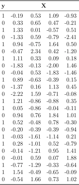
model. A logistic model regressingy on all four predictors does not converge due to separation. . . 57 Table 3.3 Comparison of estimators for the toy dataset in Table 3.2. The

tuning parameter for both ridge regression and LASSO was chosen by five-fold cross validation. For GCLS τ = 0.5 . . . 58 Table 4.1 The standardized CLS coefficients and corresponding pseudo test

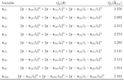
statistics for the diabetes example. The coefficients and pseudo test statistics are computed using the full CLS fit with τ = 0.5. . . 63 Table 4.2 The first step in constructing the CLS forward addition sequence

for the diabetes example. The variable under consideration, the corresponding objective function, and the value of the objective function evaluated at the CLS estimate are presented. . . 67 Table 4.3 The second step in constructing the CLS forward addition sequence

for the diabetes example. The variable under consideration, the corresponding objective function, and the value of the objective function evaluated at the CLS estimate are presented. . . 68 Table 4.4 The four variable orderings based on CLS for the diabetes

exam-ple. The CLS, CLS-T, CLS forward addition, and CLS backward elimination sequences are computed withτ = 0.5. . . 69 Table 4.5 Variable rankings for the diabetes example based on the four CLS

(11)

List of Figures

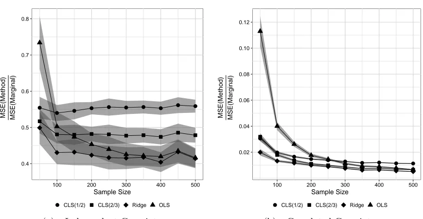
Figure 2.1 Comparison of MSE when n > p. The ratio of the MSE for each method to that of the univariate marginal estimator, and associated 95% confidence band, are plotted as a function of the sample size when the Theoretical R2 _{= 0}_._{6 and} _p _{= 20 with six important}

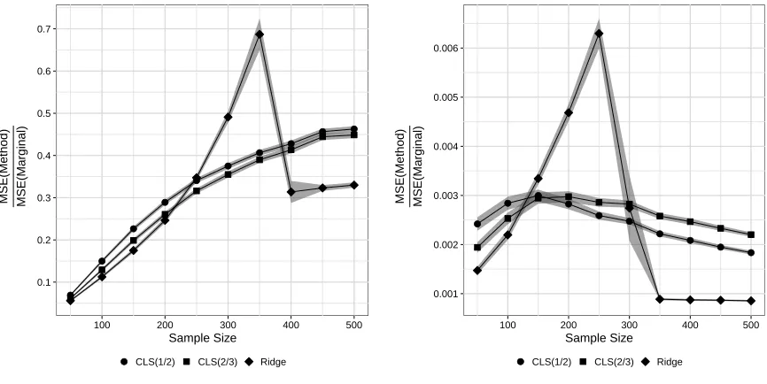
predictors. The MSE was based on 100 replicates. . . 35 Figure 2.2 Comparison of MSE when p > n. The ratio of the MSE for each

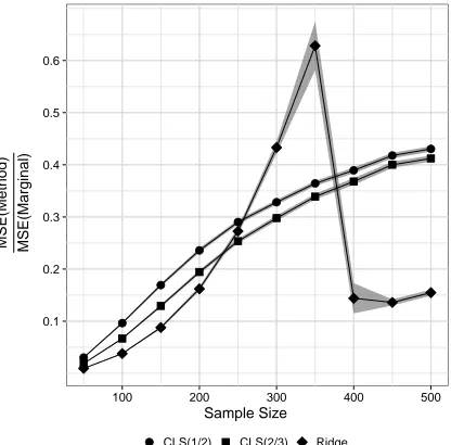
method to that of the univariate marginal estimator, and associated 95% confidence band, are plotted as a function of the sample size when the Theoretical R2 = 0.6 and p = 500 with six important predictors. The MSE was based on 100 replicates. . . 37 Figure 2.3 Comparison of MSE when p > n for important and unimportant

predictors separately. The ratio of the MSE for each method to that of the univariate marginal estimator, and associated 95% confidence band, are plotted as a function of the sample size when the TheoreticalR2 = 0.6 andp= 500 with six important predictors. The MSE was based on 100 replicates. . . 38 Figure 2.4 Ridge and CLS trace for the diabetes dataset. The value of the

standardized coefficient for each predictor is plotted over the range of possible tuning parameters, ν ∈[0,∞) for ridge regression and

τ ∈[0,1] for CLS. . . 40 Figure 3.1 Comparison of MSE in logistic regression when data is subject to

separation. The ratio of the MSE for each method to that of the LASSO estimator, and associated 95% confidence band, are plotted when n= 24 and p= 4. The MSE was based on 100 replicates. . . 58 Figure 3.2 Comparison of MSE in logistic regression when p > n. The ratio

of the MSE for each method to that of the LASSO estimator, and associated 95% confidence band, are plotted when n = 200 and

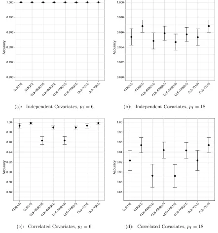
p= 500 with six important predictors. The MSE was based on 100 replicates. . . 59 Figure 4.1 Accuracy of CLS ordering procedures. The accuracy and associated

95% confidence interval are shown for each CLS ordering method when n = 500,p= 50, and the Theoretical R2 _{= 0}_._{6. Two different}

correlation structures for the predictors and two choices for the number of important predictors pI are shown. The accuracy was

(12)

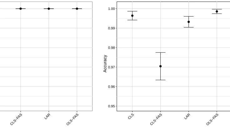
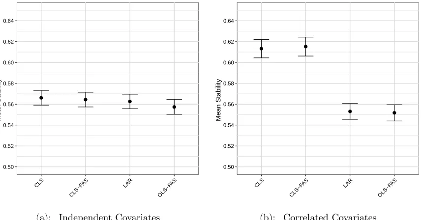
Figure 4.2 Accuracy of ordering procedures when n > p. The accuracy and associated 95% confidence interval are shown for each procedure when n = 500, p= 50, and the Theoretical R2 = 0.6. The accuracy was based on 100 replicates. . . 79 Figure 4.3 Mean stability of ordering procedures when n > p. The mean

stability and associated 95% confidence interval are shown for each procedure when n = 500, p = 50, and the Theoretical R2 _{= 0}_._6.

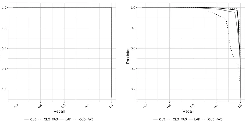
The mean stability was based on 50 bootstrap datasets across 100 replicates. . . 80 Figure 4.4 Precision-Recall curves for each ordering procedure when n > p.

The average Precision-Recall curve is shown for each procedure when n = 500, p= 50, and the Theoretical R2 = 0.6. The mean precision and recall for each point was based on 100 replicates. The Monte Carlo standard error ranged from 0 to 0.013 and from 0 to 0.014 for precision and recall, respectively. . . 81 Figure 4.5 Accuracy of ordering procedures when p > n. The accuracy and

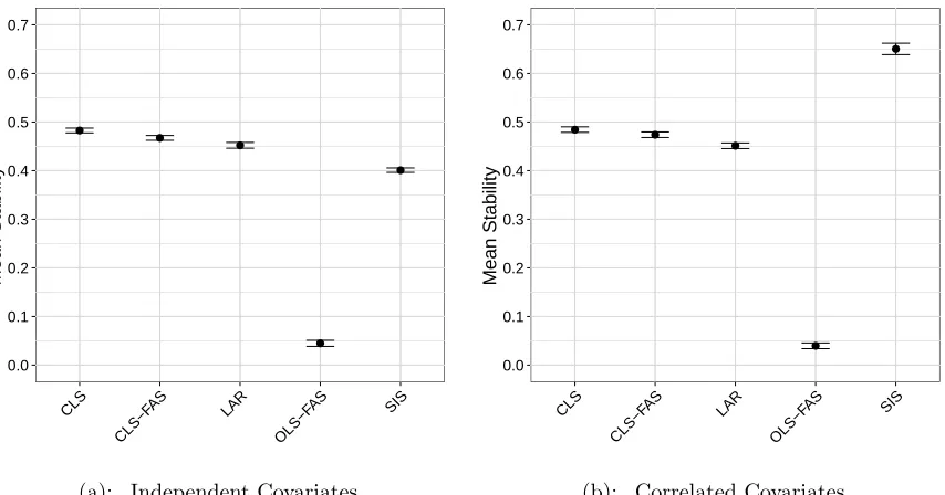
associated 95% confidence interval are shown for each procedure when n = 50, p= 500, and the TheoreticalR2 = 0.6. The accuracy was based on 100 replicates. . . 82 Figure 4.6 Mean stability of ordering procedures when p > n. The mean

stability and associated 95% confidence interval are shown for each procedure when n = 50, p = 500, and the Theoretical R2 = 0.6. The mean stability was based on 50 bootstrap datasets across 100 replicates. . . 83 Figure 4.7 Mean c-index for each ordering procedure whenp > n. The average

c-index and associated 95% confidence interval are shown for each procedure when n = 50, p = 500, and the Theoretical R2 _{= 0}_._6.

The mean c-index was based on 100 replicates. . . 84 Figure 4.8 Precision-Recall curves for each ordering procedure when p > n.

The average Precision-Recall curve is shown for each procedure when n = 50, p= 500, and the Theoretical R2 = 0.6. The mean precision and recall for each point was based on 100 replicates. The Monte Carlo standard error ranged from 0 to 0.050 and from 0 to 0.023 for precision and recall, respectively. . . 85 Figure 4.9 Predictive ability of selected models. The ratio of the mean model

error for the true model to that of the selected model for each procedure, along with its 95% confidence interval, is shown. The data correspond to n = 500, p= 50, and a Theoretical R2 _{= 0}_._6.

(13)

Figure 4.10 Selection capability of variable selection procedures. The average value of G2_{, along with its 95% confidence interval, is shown for}

each procedure. The data correspond to n = 500, p = 50, and a Theoretical R2 _{= 0}_._{6. The mean}_G2 _{was based on 100 replicates. .} ₉₂

Figure 4.11 Mean false selection rate. The average false selection rate, along with its 95% confidence interval, is shown for each procedure. The data correspond to n = 500, p= 50, and a Theoretical R2 _{= 0}_._6.

The mean false selection rate was based on 100 replicates. . . 93 Figure 4.12 Average size of selected models. The average model size, along with

its 95% confidence interval, is shown for each procedure. The data correspond to n = 500, p= 50, and a Theoretical R2 _{= 0}_._{6. The}

average model size was based on 100 replicates. . . 94 Figure 4.13 Performance of CLS based variable selection procedures

imple-mented with traditional FSR methodology. Four summaries are shown for each procedure: the ratio of the mean model error for the true model to that of the selected model, the meanG2, the mean false selection rate, and the mean model size. For each summary the 95% confidence interval is also shown. The data correspond to

n = 500, p = 50, and a Theoretical R2 = 0.6. The mean values were based on 100 replicates. . . 95 Figure 4.14 Mean c-index for each choice of τ when p > n. The average

c-index and associated 95% confidence interval are shown for the CLS sequence under various choices of τ whenn = 50,p= 500, and the Theoretical R2 _{= 0}_._{6. The mean c-index was based on 100 replicates. 97}

Figure 4.15 Predictive ability of selected models. The ratio of the mean model error for the true model to that of selected model from each proce-dure, along with its 95% confidence interval, is shown. The data correspond to n = 50, p= 500, and a Theoretical R2 = 0.6. The model error was based on 100 replicates. . . 102 Figure 4.16 Selection capability of variable selection procedures. The average

value of G2, along with its 95% confidence interval, is shown for each procedure. The data correspond to n = 50, p = 500, and a Theoretical R2 _{= 0}_._{6. The mean}_G2 _{was based on 100 replicates. .} ₁₀₃

Figure 4.17 Selection capability of variable selection procedures. The average value of G2_{, along with its 95% confidence interval, is shown for}

(14)

Figure 4.18 Accuracy of CLS and SIS ordering procedures. The accuracy and associated 95% confidence band are shown as a function of the sample size for the CLS and SIS orderings when the Theoretical

R2 _{= 0}_._{6. The total number of important predictors is held fixed at}

six. The accuracy was based on 100 replicates. . . 105 Figure 4.19 Mean index of CLS and SIS ordering procedures. The average

c-index and associated 95% confidence band are shown as a function of the sample size for the CLS and SIS orderings when the Theoretical

R2 = 0.6. The total number of important predictors is held fixed at six. The mean c-index was based on 100 replicates. . . 106 Figure 5.1 Accuracy of ordering procedures in two-stage studies. The accuracy

and associated 95% confidence interval are shown for each procedure whenn = 500,p= 50, the Theoretical R2

y = 0.4 and the Theoretical R2

r = 0.3. The accuracy was based on 100 replicates. . . 128

Figure 5.2 Accuracy of ordering procedures in two-stage studies. The accuracy and associated 95% confidence interval are shown for each procedure whenn = 500,p= 50, the Theoretical R2

y = 0.4 and the Theoretical R2_r = 0.6. The accuracy was based on 100 replicates. . . 129 Figure 5.3 Mean c-index for the ordering procedures in two-stage studies. The

mean c-index and associated 95% confidence interval are shown for each procedure when n = 500, p = 50, the Theoretical R2_y = 0.4 and the TheoreticalR2

r = 0.3. The mean c-index was based on 100

replicates. . . 130 Figure 5.4 Mean c-index for the ordering procedures in two-stage studies. The

mean c-index and associated 95% confidence interval are shown for each procedure when n = 500, p = 50, the Theoretical R2

y = 0.4

and the TheoreticalR2_r = 0.6. The mean c-index was based on 100 replicates. . . 131 Figure 5.5 Precision-Recall curves for the ordering procedures in two-stage

studies. The mean precision-recall curve and associated 95% confi-dence band are shown for each procedure when n = 500, p = 50, the TheoreticalR2

y = 0.4 and the TheoreticalR2r = 0.3. The mean

(15)

Figure 5.6 Precision-Recall curves for the ordering procedures in two-stage studies. The mean precision-recall curve and associated 95% confi-dence band are shown for each procedure when n = 500, p = 50, the TheoreticalR2

y = 0.4 and the TheoreticalR2r = 0.6. The mean

precision and recall were based on 100 replicates. The Monte Carlo standard error ranged from 0 to 0.051 and from 0 to 0.021 for precision and recall, respectively. . . 133 Figure D.1 Accuracy for the ordering procedures for two-stage studies as a

function of the parameters in the missingness mechanism. The accuracy is shown for each procedure when n = 500, p= 50, the Theoretical R2

y = 0.4 and the Theoretical R2r = 0.6. The accuracy

(16)

CHAPTER

1

Introduction

Variable selection in regression is at the root of several questions driving current medical research. What are the risk factors associated with heart failure? Which genetic biomarkers offer early identification of individuals more likely to develop cancer? When triaging a stroke victim in the emergency room, which characteristics on their medical chart are predictive of a recurrent stroke, impacting the course of treatment? Addressing each of these questions requires the researcher to distinguish the informative variables (those associated with the response of interest) from the uninformative variables.

Methods for automating the variable selection process have been the focus of much research, and many new methods have been established. However, these methods can perform poorly and be computationally difficult to implement when the number of potential predictors exceeds the sample size. Suchhigh-dimensional settings are becoming more common. For example, genetic datasets can consist of tens of subjects with thousands of variables recorded for each subject.

(17)

In this thesis, we present a new method of estimating the parameters for a generalized linear model, called Complete Least Squares. After developing this estimator extensively for the linear model, we examine its merit as a variable screening technique and as a variable selection method. The performance of the proposed screening technique is compared to others found in the literature using a simulation study.

The second part of the thesis considers variable selection in the presence of missing predictors. Specifically, we consider variable selection for two-stage studies. These retrospective studies use outcome dependent sampling schemes when collecting covariate information in an effort to reduce costs. Two-stage studies result in some covariates being unobserved for a portion of the subjects in the study. We present results from a simulation study comparing two new approaches to variable selection for two-stage studies.

In Chapter 2 we introduce the Complete Least Squares estimator for the linear model. We discuss the properties of this new estimator in detail and establish its connection to the well known ridge regression estimator. Chapter 3 extends the method of Complete Least Squares to the generalized linear model framework. In particular, we discuss the potential for handling complete separation in logistic regression via the Complete Least Squares estimator. In Chapter 4, we develop a variable selection method and screening technique for the linear model based on Complete Least Squares. In Chapter 5, we introduce two new methods for variable selection in two-stage studies. We extend these methods to the more general problem of variable selection in the presence of missing data. The remainder of Chapter 1 provides an introduction to variable selection and screening and motivates our work in subsequent chapters.

1.1 Application to Substudies in Cardiovascular Clinical

Trials

(18)

for further investigation.

It is important to note that patients included in a substudy are often not a represen-tative sample. For example, patients are not randomized to undergo revascularization; instead, revascularizations occur at the discretion of the physician. Therefore, inference restricted to the subset of patients enrolled in the substudy requires special attention if the results are to generalize to the population under study in the trial.

Following the conclusion of the trial, investigators are often interested in using the data to develop a risk model for the primary endpoint and the patient population under study. That is, researchers are interested in determining which factors are associated with an increased risk of mortality.

A number of issues arise regarding the use of variable selection methods when some of the potential predictors were only collected for the patients in the substudy. These variables are only observed for a portion of the sample and are missing for those patients not enrolled in the substudy. Furthermore, the substudy is not a representative sample. In Chapter 5, we consider variable selection in this context.

Suppose a substudy was conducted to identify genetic factors useful for identifying which patients would benefit most from treatment. Due to the expense of collecting genetic data, the substudy might consist of a few hundred patients. The genetic data, however, could yield tens of thousands of predictors for each subject. In this high-dimensional setting, variable screening prior to variable selection could improve the performance of the variable selection algorithm. We discuss a new technique for variable screening in Chapter 4.

1.1.1 PURSUIT Trial

(19)

(Boersma et al. 2000). Such risk stratification is used to determine course of treatment. The potential predictors considered by Boersma et al. (2000) included demographic data, prior medical history, prior medication, and presenting characteristics collected at randomization.

However, characteristics such as left ventricular ejection fraction and percent stenosis were not included, as these were only available for patients who underwent a diagnostic catheterization during their initial hospitalization. Approximately 50% of patients under-went this procedure during the first seven days of the trial. As a result, these variables are subject to missingness on half of the sample.

Undergoing a diagnostic catheterization was at the discretion of the physician. There-fore, the subset of patients receiving this procedure is not necessarily a representative sample from the population of interest. These patients might have been sicker, provoking their physician to order additional testing, including the catheterization.

There is an interest in determining which patient characteristics are risk factors for 30-day death or MI, allowing the risk factors to potentially include variables collected during diagnostic catheterization. If we consider those patients undergoing a diagnostic catheterization as a substudy, we can frame this problem as variable selection for a two-stage study, as discussed in Chapter 5.

1.2 Variable Selection

Frequentist variable selection methods can be broadly categorized as classical orpenalty methods. In this section, we review the key developments within each category as they relate to our work. A more comprehensive review of these methods is given by Miller (2002). For a review of Bayesian methods, see O’Hara and Sillanp¨a¨a (2009).

For illustrative purposes, consider the familiar linear mean model

E[y|X] =Xβ=x(1)β1+x(2)β2+· · ·+x(p)βp, (1.1)

where y= (y1, y2, . . . , yn)

>

is the vector of responses, X is the (n×p) design matrix of potential predictors with the j-th column given by x(j), and β is an unknown (p×1)

(20)

1. Determine a subset of variables that accurately predicts the response.

2. Determine the sparsity pattern for β — distinguish between the zero and nonzero elements.

We focus primarily on the second goal. Therefore, if the model in Equation (1.1) is assumed for the response of interest, predictors corresponding to a nonzero coefficient are considered informative (or important). In contrast, predictors corresponding to a coefficient of zero are uninformative (or unimportant).

1.2.1 Classical Methods

A closely related problem to variable selection is choosing the “best” model from a small candidate list. In variable selection, the candidate list of models is large, consisting of all possible subsets of the potential predictors. For even a small number of predictorsp, the number of possible subsets 2p _{can be unmanageable. Many classical variable selection}

methods, therefore, develop a smaller candidate list, and then choose a model from this smaller list based on some criterion.

Forward and backward selection are two methods for generating, and selecting from, a list of candidate models. Forward selection begins with an intercept-only model and sequentially adds one variable at a time to the existing model. Backward selection begins with the full model (containing all potential predictors) and sequentially removes one variable at a time from the existing model. We note that backward selection can only be applied when the number of potential predictors pis smaller than the sample size n.

At each step in forward selection, thep-value for testing whether the model is improved through the inclusion of a variable (from an F-test, for example) is computed for each of the remaining candidate predictors. The variable corresponding to the smallest of these p-values is added to the model. We refer to thep-value for the selected variable as the “p-value-to-enter.” Through sequentially adding another predictor at each step, a candidate list of nested models is generated.

(21)

with a cutoff of α = 0.05 would select Model II. It is the largest model for which all

p-values to enter are less than 0.05.

Table 1.1: Example of forward selection. For each model, the variable added to create the current model and the corresponding p-value-to-enter are given.

Model Variable Added p-value-to-enter

Model I Age 0.001

Model II Weight 0.030

Model III Height 0.063

Model IV Heart Rate 0.025

Model V Smoking Status 0.361

While this is the most common implementation of forward selection, several variations exist. One of interest to us is selecting the model using the Akaike information criterion (AIC). Let `(β,y,X) represent the loglikelihood of β given the response y and design

matrix X. The AIC is then given by

AIC =−2`(βb,y,X) + 2k,

where βb is an estimate of β and k is the dimension ofβb (the number of parameters in

the model).

(22)

criterion for choosing the next variable differs from that of forward selection; therefore, the resulting resulting list of candidate models is different.

Several limitations of these “stepwise” methods have been noted over the years. First, the order in which the variables enter (leave) the model in forward (backward) selection is not necessarily indicative of importance. As Hocking (1976) pointed out, for example, the first variable chosen in forward selection may be the first variable eliminated in backward selection. Another limitation is that the candidate list generated may not include the true model. For example, suppose that Model III in Table 1.1 is the true underlying model. Notice that it can never be selected using forward selection. Any cutoff α that would permit Model III must necessarily permit Model IV. Similarly, suppose the true model consisted of age and heart rate. Notice that the true model does not correspond to any of the models listed in Table 1.1. Finally, Breiman (1996) and Yuan and Yang (2005) show that these stepwise methods are unstable. That is, small changes in the data can result in a different list of candidate models and therefore a different selected model.

Despite these critiques, forward and backward selection continue to be widely used in the medical literature (Walter and Tiemeier 2009; Wiegand 2010).

1.2.2 Penalty Methods

Tibshirani (1996) introduced a new method of variable selection known as the LASSO (least absolute shrinkage and selection operator), which launched a series of methods for variable selection based on penalization (or “shrinkage”). Recall that ordinary least squares for the linear model estimates β by minimizing the objective function ky−Xβk2_.

Penalty methods estimate β by minimizing a penalized version of the least squares objective function,

ky−Xβk2₊_ρ₍_β₎_, _(1.2)

where the form of the penalty function ρ(·) determines the method. The LASSO solution, for example, chooses ρ(β) =λPp

j=1|βj| (Tibshirani 1996), where βj is the j-th element

of β and λ is thetuning parameter or penalty term.

(23)

Each of the penalty methods have a common approach: through penalizing the objective function, some parameters are set exactly equal to zero. Therefore, variable selection is a byproduct of the shrinking process. The level of penalization, and therefore the selected model, is controlled through the choice of the tuning parameterλ.

There are a variety of ways to choose λ. Two commonly proposed methods are the Bayesian (or Schwarz) information criterion (BIC) and cross-validation. BIC is defined similarly to AIC. If `(β,y,X) represents the loglikelihood, then the BIC is given by

BIC =−2`(βb,y,X) +klog(n),

where βb is an estimate of β, k is the dimension of βb (the number of parameters in the

model), andn is the sample size. For each value of the tuning parameter λ considered, the BIC for the resulting model is computed. The model corresponding to the smallest BIC is chosen.

The idea of cross-validation is to split the data into multiple pieces, using a por-tion of the data to build (or “train”) the model and the remainder to validate the model. K-fold cross-validation randomly partitions the data into K distinct subsets: (y,X)1,(y,X)2, . . . ,(y,X)K. For a given integer 1≤k≤K, let (y,X)−k represent the

complete data excluding those observations in (y,X)k. For each value of the tuning

parameter λ, the model is fit on the data (y,X)−k and then used to predict the response

for the data (y,X)k; the process is repeated for each value of k.

When the model fit is applied on the validation sample (y,X)k, some measure of

predictive ability is computed. For example, in linear regression, the prediction error (Tibshirani 1996) might be used. For logistic regression, the misclassification rate is a potential criterion. The value of λ, and hence the resulting model, is chosen to optimize the criterion selected.

(24)

1.2.3 False Selection Rate Methodology

Both the classical stepwise and the penalty methods rely on the choice of a tuning parameter (though stepwise methods traditionally fixed the tuning parameter a priori). The procedures commonly used to tune penalty methods (BIC and cross-validation) focus on the predictive ability of the resulting model. As our examples highlighted, prediction is only one goal in variable selection. An equally important goal is correct identification of important predictors. This latter goal motivated research in the area of tuning variable selection to improve selection capability. While a few different methods in the same spirit have been developed (Luo et al. 2006; Boos et al. 2009; Lysen 2009), we lean heavily on the false selection rate methodology of Wu et al. (2007).

Wu et al. (2007) proposed a general methodology for choosing the tuning parameter of a variable selection method by augmenting the design matrix with phony/noise variables and tracking how often these phony variables enter the final model. The tuning parameter is adjusted to achieve a specified target γ0 for the false selection rate (FSR)

γ =E

U(y,X) 1 +S(y,X)

,

where U(y,X) is the number of uninformative variables in the final model, S(y,X) is the total number of variables in the final model (excluding the intercept), and the expectation is with respect to repeated sampling of the true model. Wu et al. (2007) note that the 1 is added in the denominator to avoid division by zero, and because most models include an intercept.

Consider a variable selection method with a tuning parameter α ∈[αmin, αmax] such that the model size is monotone increasing inα. Let U(α) =U(y,X) andS(α) =S(y,X) for a specified α. As U(α) is unknown, it must be estimated. Wu et al. (2007) propose estimating U(α) by (p−S(α))θb(α), where (p−S(α)) estimates the total number of

unimportant predictors in the dataset and θb(α) is an estimate of the rate unimportant

variables enter the model. Boos et al. (2009) argue that the estimate (p−S(α)) is reasonable in the vicinity of an appropriate α.

The estimate θb(α) is obtained by appendingp phony variables to the original set of

(25)

the model is equal to the rate at which the true unimportant variables enter the model,

b

θ(α) = ¯UP(α)/p, where ¯UP is the mean number of phony variables that enter the model

over the B replicates.

With the estimate of U(α) and θ(α), the estimate of the proper tuning parameter is given by

b

α= sup

α≤α∗

{α:_bγ(α)≤γ0}, (1.3)

where

b

γ(α) = (p−S(α))θb(α)

1 +S(α) , (1.4)

andα∗ is the value ofα such that _bγ(α∗)≥γ_b(α) for allα ∈[αmin, αmax]. This choice of α∗

overcomes the fact thatγ_b(α) will decrease asα becomes large since S(α) will approachp

(Boos et al. 2009).

The phony variables generated at each of the B replications are created by randomly permuting the rows of the original design matrixX. Lysen (2009) discusses the benefits of creating phony variables in this manner. Boos et al. (2009) introduced a way of avoiding phony variables in the case of forward selection with tuning parameter “α-to-enter,” called Fast FSR. The key to this approach is setting bθ(α) = α.

1.3 Variable Screening

Variable selection methods classify potential predictors as important or unimportant. When the number of potential predictorspfar exceeds the sample sizen, variable selection methods can misclassify the predictors (Fan and Lv 2008). In the literature, there are two dominating approaches to handling these high-dimensional cases: variable screening followed by selection, and simultaneous dimension reduction and selection. We focus on the former; for an example of the latter, see Bondell and Li (2009)

Variable screening is a step applied prior to a variable selection algorithm. The goal of the screening step is to eliminate from the candidate list those predictors that exhibit the least evidence of being important. The variable selection algorithm of choice is then applied to this reduced list to select the final model.

(26)

the higher the corresponding rank. The top k variables are then retained for variable selection. Fan and Lv suggested choosing k =n/log(n), k =n−1, ork =αnfor some

α∈(0,1), where n is the sample size.

Fan and Lv also gave conditions under which SIS enjoys the sure screening property. That is, the probability that the screening step retains the important variables approaches 1 as the sample size grows. To establish this property, Fan and Lv assumed the correlation among the predictors does not become too large. SIS performs best when the predictors are independent.

If the predictors are highly correlated, Fan and Lv suggested an iterative version of SIS (ISIS) be used. However, this procedure does not enjoy the simplicity of SIS. Since its development, SIS has been extended to the generalized linear model framework (Fan et al. 2009; Fan and Song 2010). Fan and Lv (2010) discuss the use of various variable selection techniques in conjunction with SIS.

As an alternative to SIS, Wang (2009) considered using the sequence generated by forward selection as a technique for variable screening. This method is referred to as forward regression screening. While the entire sequence generated by forward selection cannot be obtained when p > n, a partial list consisting of the first n−1 models can be obtained. Wang suggests retaining the first k ≤n−1 variables that enter the model using the forward sequence, where k is chosen using a version of BIC.

Under various assumptions, Wang (2009) established that BIC moderated forward regression screening enjoys the sure screening property. The simulation results presented by Wang suggest that forward regression screening retains a very small number of predictors. To include a larger pool of candidate predictors in the selection stage, it is possible to consider choosingk larger than that suggested by the BIC used by Wang. However, the proof for the sure screening property assumes the use of this BIC.

Similar to Fan and Lv (2008), Wang considers applying a variable selection method to thek variables retained during the screening step. However, note that choosing k via BIC is itself a variation on the classical forward selection method. Therefore, the procedure proposed by Wang is akin to performing variable selection twice. The first pass is used for screening, while the second pass is used to select the final model.

(27)

Wang (2009) and Fan and Lv (2008), Wasserman and Roeder proposed using hypothesis testing to select the final model from the reduced candidate list.

1.4 Variable Selection in Two-Stage Studies

The preceding discussion of variable selection methods assumed that the response and covariate data were fully available for all observations. However, in many practical situations (the substudies in Section 1.1, for example) complete data are available only for a subset of observations. For substudies in cardiovascular clinical trials, the subjects not enrolled into the substudy are missing those covariates collected during the substudy. That is, the missing data occurs for a block of subjects. This pattern of missingness is also observed in two-stage studies.

In the first phase of a two-stage study, the response and a set of predictors are collected for all subjects. A subset of the patients enrolled are then sampled into a second phase (like selecting patients for a substudy) in which additional covariates are collected. The additional covariates are therefore unobserved for those subjects not sampled into the second phase. We discuss this design in more detail in Chapter 5.

When subjects are not randomly sampled into the second phase, inference must be performed with caution as parameter estimates can become biased. This is a well-studied problem (Zhao and Lipsitz 1992; Zhou et al. 2011). Inference in two-stage studies is usually conducted using conditional moment estimation (commonly referred to as the “Breslow and Cain” approach, Breslow and Cain 1988) and inverse probability weighting (Zhao and Lipsitz 1992; Robins et al. 1994). Conditional moment estimation makes use of the conditional distribution of the observed data for inference. Inverse probability weighting uses semiparametric theory to suggest estimating equations appropriate for conducting inference.

(28)

forms of missing data due to the structure of the missing data inherent to this design. To our knowledge there has been no research conducted into variable selection in the specific context of two-stage studies. There has, however, been research into variable selection in the presence of missing data. Generalizations of selection criteria, such as AIC and BIC, that account for missingness have been established (Hens et al. 2006; Claeskens and Consentino 2008). However, these methods are directed at choosing among a small number of candidate models. They do not address variable selection directly.

Other work has focused on variable selection following multiple imputation (Wood et al. 2008; Chen and Wang 2011). These methods are not directly applicable to two-stage studies as multiple imputation is not a viable method for these designs. Garcia et al. (2010) introduced a penalized approach to variable selection in the presence of missing

data. Their method, similar to multiple imputation, requires investigators to posit a model for the distribution of the predictors. Therefore, their approach is not entirely satisfactory for two-stage studies.

The most promising research with application to variable selection in two-stage studies has incorporated weighting techniques to account for the missingness. Wolfson (2011) introduced a method of variable selection for estimating equations. As we discuss in Chapter 5, weighting methods for two-stage studies are implemented via estimating equations. While Wolfson (2011) recognized the potential of his method for variable selection in the presence of missing data, this was not the primary objective of his paper. As a result, his simulation results for missing data scenarios are limited in scope.

Ziegler (2006) presented a thorough discussion of modern variable selection methods in a variety of missing data scenarios. We note two drawbacks of her work that we improve upon in the context of two-stage studies. First, she did not integrate methods for handling missing data with variable selection methods. Instead, she concentrated on the performance of these methods when applied to the complete cases alone. Second, her primary interest was on estimation of the parameters in the final model. We focus on developing a method that can correctly identify the sparsity pattern.

1.5 Summary

(29)

ridge regression.

We study the merits of CLS for both variable selection and variable screening. Com-pared to other variable selection methods that produce lists of variables ordered by estimated importance (such as forward selection), CLS is more stable, but less accurate. In our work, stability is a measure of the variation in the variable ordering due to per-turbations in the data. Accuracy is a measure of the variation in the variable ordering across repeated sampling from the underlying true model.

As a tool for variable screening, CLS is shown to be generally competitive with the most commonly-used methods. Moreover, CLS is shown to have improved performance in certain modeling scenarios.

Our simulation studies suggest that further research is needed to develop practical guidelines for implementing screening. Specifically, guidelines are needed for determining the sample size required to retain the important predictors with high probability.

(30)

CHAPTER

2

Complete Least Squares

Consider estimating thep-dimensional vector of parameters β from the linear model

y=Xβ+, (2.1)

whereyis an (n×1) response vector,Xis an (n×p) design matrix, and= (1, 2, . . . , n)

> wherei are independently and identically distributed such thatE(i) = 0 andV (i) = σ2

for an unknownσ2_{. Without loss of generality, we assume} _y_and _X _{have been centered}

and scaled appropriately such that y>1= 0, y>y= 1,X>1=0, and X>X=R, where R is a valid correlation matrix.

It is well known that the Ordinary Least Squares (OLS) estimator

b

β_OLS = arg min_βky−Xβk2

(31)

Complete Least Squares (CLS). We show that the CLS objective function, similar to ridge regression and LASSO, leads to a biased estimator for β. We compare the form of the CLS estimator with similar estimators found in the literature, and we investigate its properties.

2.1 Motivating the Objective Function

As their primary example of implementing the LASSO using the LARS algorithm, Efron et al. (2004) presented data from a study following 442 diabetic patients. The data included each patient’s age (x(1)), body mass index (BMI, x(2)), average blood pressure

(BP,x(3)), and the response of interesty— “a quantitative measure of disease progression

one year after baseline.” Our goal is to construct an estimate of β= (β1, β2, β3)

> , the parameters corresponding to age, BMI, and BP, respectively.

With so few variables, we can list the objective functions corresponding to all possible linear models comprised of the three variables age, BMI, and BP. If we assume that the response and predictors have been appropriately centered and scaled, then the seven possible objective functions are listed in Table 2.1.

Table 2.1: Objective functions corresponding to all possible linear models comprised of three variables. No intercept is needed in the model specification if we assume the response and covariates have been appropriately centered and scaled.

One-Variable Models: ky−x(1)β1k2

ky−x(2)β2k2

ky−x(3)β3k2

Two-Variable Models: ky−x(1)β1−x(2)β2k2

ky−x(1)β1−x(3)β3k2

ky−x(2)β2−x(3)β3k2

Three-Variable Models: ky−x(1)β1−x(2)β2−x(3)β3k2

(32)

sum of squares corresponding to the three-variable model. Without prior knowledge as to which of these seven models is correct, a reasonable alternative to OLS is to determine a value ofβ that is “good” across all seven models. To this end, consider minimizing the sum of the least squares (LS) objective functions (residual sums of squares) for all models. That is, we estimate β by minimizing

Q(β) =ky−x(1)β1k2+ky−x(2)β2k2+ky−x(3)β3k2

+ky−x(1)β1−x(2)β2k2+ky−x(1)β1−x(3)β3k2+ky−x(2)β2−x(3)β3k2

+ky−x(1)β1−x(2)β(2)−x(3)β3k2.

The function Q(β) is the CLS objective function, and the value of β that minimizes

Q(β) is the CLS estimator in this case. Intuitively, this estimate of β is “good” across all possible linear models comprised of any combination of these three variables. We now derive the CLS objective function in general and the corresponding estimator.

2.2 CLS Objective Function and Corresponding

Estima-tor

In the previous section we argued heuristically that minimizing the sum of the LS objective functions corresponding to all possible linear models provides a reasonable estimate of β. In this section we develop the CLS objective function forp variables in which we allow models of each size to be differentially weighted. We then derive the corresponding CLS estimator and discuss the effect of weighting each model size.

2.2.1 Derivation of the CLS Objective Function

In order to consider the general case ofpvariables, we introduce some additional notation. For an integer k such that 1≤k ≤p, let Sp,k denote the set of all p-dimensional vectors

with exactlyk elements taking value 1, and exactlyp−kelements taking value 0. Formally,

Sp,k=

(

s:s∈ {0,1}p _and p

X

j=1

sj =k

)

(33)

For a fixed integer k and vector s∈ Sp,k, let Ds= diag{s}. Then,

ky−XDsβk2

denotes the LS objective function for a particular linear model with k variables.

There are _kp such models of size k, each model corresponding to a single element of s∈ Sp,k. Let Qp,k(β) be the summation of the LS objective functions corresponding to

all models of size k. That is, let

Qp,k(β) = X

s∈Sp,k

ky−XDsβk2.

For example, if k =p,Qp,k corresponds to the full-model OLS objective function as there

is only one model of sizep — the full model with all variables included. Similarly, there are p models of size 1; thus, if k = 1, Qp,k corresponds to the summation of the LS

objective functions for thep models containing only a single variable. Let ω = (ω1, ω2, . . . , ωp)

>

be a set of pre-specified model weights such that ωj ≥ 0

for all j = 1,2, . . . , p. These weights allow more emphasis to be given to models of a specific size when constructing the CLS objective function and corresponding estimator. For example, we might choose to place twice as much weight on models of size two than models of size three. Given a choice of model weights ω, we define the CLS objective function by

Qp(β,ω) =

p

X

k=1

ωkQp,k(β). (2.2)

The CLS objective function is a weighted average of the LS objective functions corre-sponding to all possible models. Although seemingly very complicated, we now show that

(34)

Observe that

Qp,k(β) = X

s∈Sp,k

(y−XDsβ)

>

(y−XDsβ)

= X

s∈Sp,k

y>y−2y>XDsβ+β>DsX>XDsβ

= p k

y>y−2y>X X

s∈Sp,k

(Ds)β+β>

X

s∈Sp,k

(DsX>XDs)β.

Note that for a given s∈ Sp,k

DsX>XDs

i,i =







X>X_i,i if si = 1,

0 if si = 0,

for all i ∈ {1,2, . . . , p}. That is, the i-th diagonal element of X>X is picked off, if and only if, the i-th diagonal element of Ds is 1. Recall that by definition, there are

exactlyk elements ins that equal 1, and the remainingp−k elements equal 0. For some

i∈ {1,2, . . . , p}, fix si = 1. Of the remaining p−1 elements in s, there are exactlyk−1

elements that equal 1. As these remaining ones can occur in any of p_k−₋1₁ configurations, there are p_k−₋1₁ elements inSp,k for which si = 1. This implies that each diagonal element

of X>X appears in p_k−₋1₁ terms of P

s∈Sp,kDsX

>_XD

s. It is important to note that we

follow the convention that for any integer a, a₀

= 1 and a_b

= 0 for allb <0. Similarly, for i, j ∈ {1,2, . . . , p} wherei6=j, we have that

DsX>XDs

i,j =







X>X_i,j if si =sj = 1,

0 if si = 0 or sj = 0.

Fixing two elements insto be 1 implies that of thep−2 remaining elements,k−2 of them equal 1. Thus, there are p_k−₋2₂ elements in Sp,k for whichsi = 1 andsj = 1. This implies

that each off-diagonal element of X>X appears in p_k−₋2₂ terms of P

s∈Sp,kDsX

>_XD

s.

We then have that

X

s∈Sp,k

DsX>XDs=

p−2

k−2

X>X−D_X>_X

+

p−1

k−1

(35)

where D_X>_X is the diagonal matrix with diag (D_X>_X) = diag X>X. Note that D_s

is idempotent for any choice of s; thus, we have that Ds = DsIp>IpDs, where Ip is the

identity matrix of dimension p. Applying the result in Equation (2.3) gives

X

s∈Sp,k

Ds=

X

s∈Sp,k

DsI>pIpDs =

p−1

k−1

Ip.

Now, we have that

Qp,k(β) =

p k

y>y−2

p−1

k−1

y>Xβ

+β>

p−2

k−2

X>X−D_X>_X+

p−1

k−1

D_X>_X

β. (2.4)

This simplified form of Qp,k(β) leads to a simple expression for the CLS objective

function. Observe that

Qp(β,ω) =

p

X

k=1

ωkQp,k(β,w)

= p X k=1 ωk p k

y>y−

p

X

k=1

2ωk

p−1

k−1

y>Xβ

+β>

" _p X

k=1 ωk

p−2

k−2

X>X−D_X>_X

+ p X k=1 ωk

p−1

k−1

D_X>_X

#

β

=λ0y>y−2λ1y>Xβ+β> λ2X>X+ (λ1−λ2)D_X>_Xβ, (2.5)

where λj =

Pp

k=1ωk p

−j k−j

for j = 0,1,2. Rewriting Equation (2.5), we have

Qp(β,ω) = [λ0−pλ1+ (p−1)λ2]y>y

+λ2Qp,p(β) + (λ1−λ2)Qp,1(β). (2.6)

This form of the objective function provides insight into the corresponding estimator. The CLS estimator, the value ofβ that minimizes the CLS objective functionQp(β,ω) for a

(36)

2.2.2 CLS Estimator

Theorem 2.2.1 establishes the CLS estimator, the value of β that minimizes the CLS objective function.

Theorem 2.2.1. For a fixed set of model weights ω = (ω1, ω2, . . . , ωp)

>

such that ωj ≥0

for all j, the estimator

b

β_CLS = τX>X+ (1−τ)D_X>_X

−1

X>y

minimizes

Qp(β,ω) = p

X

k=1

ωkQp,k(β),

where τ =λ2/λ1 =Pp

k=1ωk p−2 k−2

/Pp

k=1ωk p−1 k−1

.

Proof. Observe that

Qp,k(β) = X

s∈Sp,k

ky−XDsβk2

= X

s∈Sp,k

ky−XDsβb_CLS+XD_s(βb_CLS−β)k2

= X

s∈Sp,k

(y−XDsβb_CLS)>(y−XDsβb_CLS)

+ X

s∈Sp,k

2(y−XDsβb_CLS)>XD_s(βb_CLS−β)

+ X

s∈Sp,k

h

XDs(βb_CLS−β) i>h

XDs(βb_CLS−β)

i

=Qp,k(βb_CLS) + 2

p−1

k−1

y>X(βb_CLS−β)

−2βb

>

CLS

p−2

k−2

(X>X−D_X>_X) +

p−1

k−1

D_X>_X

(βb_CLS−β)

+ X

s∈Sp,k

(37)

where the last equality follows from applying the results of Equation (2.3). Now, we have

Qp(β,ω) = p

X

k=1

ωkQp,k(β)

=Qp(βb_CLS,ω) + 2λ1y>X(βb_CLS−β)

−2βb

>

CLS

λ2X>X+ (λ1−λ2)DX>_X

(βb_CLS−β)

+ p X k=1 ωk   X

s∈Sp,k

kXDs(βb_CLS−β)k2





=Qp(βb_CLS,ω) +

p X k=1 ωk   X

s∈Sp,k

kXDs(βb_CLS−β)k2



, (2.7)

where the crossproduct term vanishes since βb_CLS solves

λ2X>X+ (λ1−λ2)D_X>_Xβ=λ1X>y.

As the last term in Equation (2.7) is always non-negative, it is clear that Qp(β,ω) is

minimized when β=βb_CLS.

2.2.3 Choice of Model Weights

The CLS estimator depends on the choice of model weights ω. In this section, we describe the resulting estimator for a few specific choices of ω.

Recall that λj = Pp_k=1ωk p_k−₋j_j

for j = 0,1,2. Observe that for any integer k such that 1≤k≤p, we have

ωk p

−2 k−2

ωk p_k−₋1₁

=

k−1

p−1 ≤1.

That is, each term comprisingλ1 is at least as large as the corresponding term inλ2. This

implies that τ =λ2/λ1 ∈[0,1].

The CLS estimator has a similar form to that of the OLS estimator, except the off-diagonal elements of X>X are scaled by τ. Through the choice of model weights ω, we alter the value ofτ and therefore control the degree to which the off-diagonal elements of X>X are scaled. Giving equal weight to models of all sizes (i.e. choosing ωj = 1

(38)

justification for differentially weighting each model size.

The full OLS fit is a special case of CLS obtained by assigning positive weight to only the model with pvariables; that is, ωp = 1 andωj = 0 for allj 6= p. This results inτ = 1

and the OLS estimator. Similarly, letting ω1 = 1 andωj = 0 for allj 6= 1, giving positive

weight to only models of size 1, results in τ = 0. This corresponds to the estimates from the univariate marginal regression models.

We consider one more choice for the model weights. The CLS objective function when ωj = 1 for all j is minimizing the average of the LS objective functions for all

possible models. This can be seen as summing in two directions: we sum the LS objective functions for all models of size k; then, we add these sums across all model sizes. Using this procedure, more emphasis is naturally given to models with p/2 variables as there are more models of this size. Instead of summing in two directions, consider summing an average: we average the LS objective functions for all models of size k; then, we sum these averages across all model sizes. That is, choose ωk =

p

k

−1

. Then ωkQp,k(β) is

the average of the LS objective functions for models of size k. It is straightforward to show that this choice of ω results inτ = 2/3. It should be noted that if X is orthogonal, the CLS estimator is the same for all choices of τ and reduces to the OLS estimator, which is also obtained by minimizing the univariate marginal models.

As stated above, τ controls the degree to which the correlation between the predictors X contributes to the estimation of β. Before discussing the effects of τ, we briefly discuss several related estimators in the literature.

2.3 Related Estimators

If the number of variablesp is larger than the sample size n, X>X is singular. Even if

(39)

The introduction of penalty (or “shrinkage”) methods, such as ridge regression (Hoerl and Kennard 1970) and LASSO (Tibshirani 1996), offered alternatives to ordinary least squares. Through additional restrictions on the OLS objective function, these approaches result in estimators that do not suffer from the same limitations as OLS when X>X is ill-conditioned. A group of these penalized estimators, ridge regression and several generalizations, closely resemble the CLS estimator.

Hoerl and Kennard (1970) introduced ridge regression as a method of estimation for non-orthogonal regression problems. They proposed penalizing the OLS objective function in such a way that the resulting estimator, though biased, would have a smaller mean squared error than that of OLS. The ridge estimator βb_Ridge is the value of β that

minimizes

ky−Xβk2₊_ν_k_β_k2_, _(2.8)

where ν ≥0 is a tuning parameter. The concept behind ridge regression is “regression toward the mean.” When the OLS estimates may be unreliable (as described above), the tuning parameter can be used to constrain the parameters from becoming too large; this results in an estimate of the conditional mean of y that is closer to the observed average response. From the form of the ridge estimator for a particular choice ofν,

b

β_Ridge(ν) = X>X+νIp

−1

X>y,

it is clear that smaller values of the tuning parameter result in estimates closer to OLS. As the tuning parameter increases, the parameter estimates approach 0.

It is readily apparent that the form of the ridge estimator is similar to the CLS estimator. For a direct comparison, observe that if we assume thatXhas been appropriately centered and scaled, then D_X>_X=I_p, which allows us to rewrite the CLS estimator as

b

β_CLS =τX>X+ (1−τ)Ip

−1

X>y =τ−1X>X+ (τ−1−1)Ip

−1

X>y = (1 +ν)βb_Ridge(ν),

where we have defined ν = (τ−1₋_{1). Thus, for a given penalty} _ν_{, there is a corresponding}

(40)

Further, as ν = (τ−1₋₁₎_≥_{0, the CLS estimator is an inflated ridge estimator. We will}

discuss the effect of this inflation factor in more detail in Section 2.4; for now, we simply note that this inflation factor prevents the estimates from shrinking toward 0.

While the ridge and CLS estimators share a similar form, they differ in the choice of tuning parameter. The CLS tuning parameter τ is a function of weights applied to various model sizes in the objective function. In contrast, the ridge tuning parameterν is typically chosen from data-driven methods, such as a ridge trace (Hoerl and Kennard 1970) or generalized cross validation.

Lipovetsky (2006) considered extending ridge regression by adding additional penalty functions to Equation (2.8). Lipovetsky’s “ridge-2” estimator βb_Ridge₋₂ is the solution to

the penalized regression

ky−Xβk2+η1kβk2+η2kX>y−βk2+η3ky>(y−Xβ)k2.

The first penalty function corresponds to that of ridge regression and will shrink the estimates toward 0. The second penalty “shrinks” the estimates toward those from the univariate marginal fits. Here we use “shrink” loosely as the marginal estimates may actually be larger in magnitude than the OLS estimates. Lipovetsky (2006) argues that shrinking toward the marginal estimates stabilizes the fit from the resulting estimator. In ridge regression, as the penalty term increases toward infinity, the quality of fit diminishes. However, as η1 increases, the second penalty stabilizes the fit while allowing the estimator

to overcome the effects of an ill-conditioned X>X matrix. The third penalty constrains the sums of squares in order to maximize the coefficient of determination R2.

The resulting estimator is

b

β_Ridge₋₂ =ν1 X>X+ν2Ip

−1

X>y,

where ν1, ν2 ≥ 0 are functions of η1, η2, and η3. It is important to note that ν1 can be

chosen independently ofν2. Therefore, while the ridge-2 estimator is proportional to the

(41)

parameter is a function of model weights.

Lipovetsky (2010) developed another extension to ridge regression, termed “enhanced ridge regression,” based on minimizing a new objective function

ηky−Xβk2_{+ (1}₋_η₎ X

s∈Sp,1

kp−1y−XDsβk2,

where η∈[0,1] andp is the number of predictors. This is extremely similar to the form of the CLS objective function given in Equation (2.6). It should not be a surprise that the resulting estimator,

b

β_Ridge−E = (1 +ν/p) X

>

X+νIp

−1

X>y,

has a form similar to the CLS estimator, where ν = (η−1₋₁₎_≥_{0. Again, this estimator}

is proportional to the ridge estimator. However, we notice two distinct differences between the ridge enhanced estimator and the CLS estimator. First, the inflation factor for the ridge enhanced estimator is smaller than that for CLS. Second, the choice of the tuning parameter η is not informed by model weights as τ is for the CLS estimator.

While Lipovetsky constructed estimators similar to the CLS estimator, we note that neither resulted from considering a weighted sum of all possible LS objective functions. It is this weighted sum (see Equation (2.5)) that informs the penalty term in the CLS estimator.

In these penalty methods, the effect of the tuning parameter on the estimates was gleaned from the form of the penalty function. We now develop some notation that will shed some light on the effect of the tuning parameter τ in CLS.

2.4 CLS: Shrinking the Estimates Toward the Marginal

Through a transformation of the regression problem, we are able to gain some insight into the effect of τ in CLS. We show that unlike ridge regression or the LASSO, which shrink the coefficients toward 0, the CLS estimates are pulled toward the estimates obtained from the univariate marginal regression models. As a consequence, they are unbiased in the special case where X>X=Ip.

(42)

that D_X>_X = I_p. Let g_j and γ_j be the j-th eigenvector and corresponding eigenvalue,

respectively, of X>X, for j = 1,2, . . . , p. Then, observe that

τX>X+ (1−τ)Ip

gj =τ X>X

gj + (1−τ)gj

=τ γjgj + (1−τ)gj

= [τ γj+ (1−τ)]gj.

That is, the matrix τX>X+ (1−τ)Ip

has the same eigenvectors as X>X; furthermore, the corresponding eigenvalues are simply a weighted average of 1 and the eigenvalues of X>X.

Collecting the orthogonal eigenvectors and corresponding eigenvalues of X>X into matrices, consider the spectral decomposition X>X = GΓG>. Let ∆ be the (p×p) diagonal matrix for which the ratios of the original eigenvalues to the transformed eigenvalues are on the diagonal. That is, the j-th diagonal element of ∆ is given by

δj =γj/[τ γj + (1−τ)]. Then, we can write the CLS estimator as

b

β_CLS(τ) =τX>X+ (1−τ)Ip

−1

X>y = G∆−1ΓG>−1X>y

=GΓ−1∆v =Gα,

where v =G>X>y and α= Γ−1∆v. As G is free of the choice of τ, the form of the CLS estimator as a function of τ depends solely onα. Notice that thej-th element ofα

is given by

αj =

vj τ γj + (1−τ)

.

For OLS (τ = 1), αj = vj/γj. For the univariate marginal estimates (τ = 0), αj = vj.