Combined Time- and Frequency-Domain Calculations for Seismic SSI Problem

COMBINED TIME- AND FREQUENCY-DOMAIN CALCULATIONS FOR SEISMIC

SSI PROBLEM

Alexander Tyapin, Head of the Lab, Dept. of Dynamics and Seismic Safety, Atomenergoproject (Moscow), Russia (atyapin@bvcp.ru)

ABSTRACT

Specialized SSI (soil-structure interaction) software (e.g., SASSI) is able to provide floor response spectra, but it can not work with extremely fine FEM models used for the structural design. As a result, in the design models engineers have to use some primitive SSI representations like “soil” springs and dashpots distributed under the basement in the conventional platform model. The goal of the research is to propose an algorithm combining the time- and the frequency-domain calculations to enable the incorporation of the SSI wave effects into the conventional analysis and design.

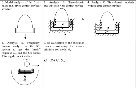
As basement slabs in the NPP structures usually are comparatively stiff, one may consider the absolutely rigid soil-structure contact surface to relate to the main part of the actual SSI forces acting from the soil to the soil-structure. The additional part of these SSI forces (resulting from the actual flexibility of the underground part of the structure) is considered to be small and can be estimated using primitive models of SSI. So, the main idea of the proposed approach is to separate the “rigid” SSI forces from the “flexible” ones. “Rigid” SSI forces are calculated by SASSI (i.e., first in the frequency domain, then in the time domain) using simplified structure model – this is called “analysis A”. Then the fine structural model resting on a rigid platform with a primitive “soil support” (distributed springs and dashpots) is analyzed in the time domain. The dynamic excitation goes not from the platform movement, as usually, but from the external excitation forces distributed over the soil-structure contact surface. These excitation forces are derived from the SASSI results in such a way that in case the rigid contact surface moves according to the “analysis A” results, the total forces acting on the structure from the soil (i.e., external excitation forces, forces from the “soil springs” and “soil dashpots” in the fine model) are the same as those forces in “analysis A”. As a consequence, if structural model in “analysis A” was adequate enough, the time–domain seismic response of the rigid contact surface in the fine structural model must be the same as in “analysis A”. This is specially checked by the time-domain “analysis B” of the fine structural model with artificially rigid contact surface. For the final design (“analysis C”) the same external excitation forces are applied in the time domain, but the contact surface is set flexible (i.e., free from the artificial constrains of “analysis B”). As a result, the primitive soil springs/dashpots in “analysis C” actually work only with “flexible” part of the response.

Various problems regarding the implementation of the proposed approach are outlined together with the state-of-the-art. Simple embedded structure is tested, and the errors are demonstrated. For the comparatively stiff basement the results are pretty good, though for the flexible basements the traditional platform model sometimes is better. The next step will be the investigation of the actual NPP buildings to find out, whether the new approach gives better results.

INTRODUCTION

It is well-known that the soil-structure interaction (SSI) analysis can be satisfactory performed only in the frequency domain due to the wave effects in the infinite soil. Specialized SSI software (e.g., SASSI) is able to provide floor response spectra, but it can not work with extremely fine FEM models used for the structural design. As a result, in the design models engineers have to use some primitive SSI representations like “soil” springs and dashpots distributed under the basement in the conventional platform model. The goal of the research is to propose an algorithm combining the time- and the frequency-domain calculations to enable the incorporation of the SSI wave effects into the conventional analysis and design.

GENERAL APPROACH

The general idea is as follows. Basement slabs in the NPP structures usually are comparatively stiff (vertical walls attached to the slabs contribute to the stiffness also). As a consequence, one may consider the absolutely rigid soil-structure contact surface to relate to the main part of the actual SSI forces acting from the soil to the soil-structure. The additional part of these SSI forces (resulting from the actual flexibility of the underground part of the structure) is considered to be small and can be estimated using primitive models of SSI. So, the main idea of the proposed approach is to separate the “rigid” SSI forces from the “flexible” ones. “Rigid” SSI forces are calculated by SASSI

(i.e., first in the frequency domain, then in the time domain) using simplified structure model – this is called “analysis A”. Then the fine structural model resting on a rigid platform with a primitive “soil support” (distributed springs and dashpots) is used for the time-domain analysis. The dynamic excitation goes not from the platform movement, as usually, but from the external excitation forces distributed over the soil-structure contact surface. These excitation forces are derived from the SASSI results in such a way that in case the rigid contact surface moves according to the “analysis A” results, the total forces acting on the structure from the soil (i.e., external excitation forces, forces from the “soil springs” and “soil dashpots” in the fine model) are the same as those forces in “analysis A”. As a consequence, if structural model in “analysis A” was adequate enough, the time–domain seismic response of the rigid contact surface in the fine structural model must be the same as in “analysis A”. This is specially checked by the time-domain “analysis B” of the fine structural model with artificially rigid contact surface. For the final design (“analysis C”) the same external excitation forces are applied in the time domain, but the contact surface is set flexible (i.e., free from the artificial constrains of “analysis B”). As a result, the primitive soil springs/dashpots in “analysis C” actually work only with “flexible” part of the response.

The general layout of the proposed algorithm is shown in the Fig.1.

0. Modal analysis of the fixed-based (i.e., fixed contact surface) structure

3. Analysis B. Time-domain analysis with rigid contact surface

4. Analysis C. Time-domain analysis with flexible contact surface

1. Analysis A. Frequency-domain analysis of the SSI system to get the “main” response Um and the SSI forces

R for rigid contact surface

2. Re-calculation of the excitation forces considering the chosen primitive soil model Gs

m

s

U

G

R

Q

=

+

Fig. 1. General layout of the proposed algorithm

It is more convenient to further describe the proposed method in the frequency domain. Let Cb be complex

frequency-dependent dynamic stiffness matrix of the upper structure, combining stiffness, damping and inertia. Let Db be the same matrix, but for the structure with very stiff contact surface. Let Cs be the soil dynamic stiffness

matrix for the same contact nodes. Let Gs be the same matrix, but for the primitive soil model. Further on, let U0 be

a displacement vector for the contact nodes due to the seismic excitation in the soil without structure, but after the outcropping. Finally, let U be the displacement vector for the initial structure interacting with soil, and let Um be the

same vector, but for the structure with very stiff contact surface. Then the equation for the initial structure is

)

(

U

U

C

U

C

=

−

The same equation, but for the structure with very stiff contact surface is

)

(

s m

b

U

C

U

U

D

=

−

Both sides of the Eq.2 are equal to the contact forces R in case of the structure with very stiff contact surface

)

(

s m

b

U

C

U

U

D

R

=

=

−

Putting Eq.3 into Eq.1 one gets from Eq.1

m s s

b

C

U

R

C

U

C

+

)

=

+

(

So far, the “fine” solution was considered. The author suggests changing the “fine” U for the “approximate” V, as the result of changing the “fine” soil matrix Cs for the “approximate” soil matrix Gs in both parts of the Eq.4

m s s

b

G

V

R

G

U

C

+

)

=

+

(

As a result of “Analysis A”, one obtains contact forces R and “rigid” displacements Um. Then one chooses the

“approximate” soil model Gs and recalculates the forces R to the excitation forces R+GsUm , to use them further as

the right-hand part of Eq.5. “Analysis B” does not bring the new results, but it is necessary to check the previous steps for completeness. Finally, the “Analysis C” is the target design analysis – the solution of Eq.5.

Subtracting Eq.5 from Eq.4 one gets

)

)(

(

)

(

)

(

C

+

G

U

−

V

=

G

−

C

U

−

U

In Eq.6 the error (U-V) of the approximate solution V is presented as the response of the structure with “primitive” soil model to some excitation, proportional, on one hand, to the error (Gs-Cs) in soil modeling and, on the other

hand, to the deviation of complete displacements U from “rigid” displacements Um . The stiffer is the basement, the

closer are U and Um , and the closer are U and V for the given “primitive” soil model. Thus, the proposed approach

is asymptotic. On the other hand, the better is “primitive” soil model, the better is the approximate solution for the given basement flexibility.

One should note the difference in the origin of the two terms in the right-hand part of Eq.6: the first term depends on the choice of the engineer, the second term has clear physical meaning as both U and Um are “fine” solutions (i.e,

obtained for the ”fine” soil).

TWO GROUPS OF PROBLEMS

There are two groups of problems, arising in the process of the implementation of the proposed method. The first group refers to the “Analysis A”.

1.1. To present the upper structure on the “Analysis A” in the convenient form, one should add the special frequency-dependent element to the SASSI library.

1.2. One should obtain the parameters of that special element from the results of the general–purpose FEM soft, used for the modal analysis of the fixed-based structure.

1.3. One should perform the transition from the frequency domain to the time domain with contact forces R and rigid response Um.

1.4. The FEM mesh, used in the design soft is many times denser than that used in SASSI. Thus, a separate problem is to move from the SASSI mesh to the fine mesh with forces R.

The second group of problems refers to the soil modeling in “Analysis B” and “Analysis C”.

2.1. One should investigate the influence of the basement flexibility on the seismic response in terms of internal forces in the basement to decide, whether to account for the basement flexibility at all.

2.2.In case of significant influence one should try the typical primitive soil models (e.g., uniform distribution of springs and dashpots) to estimate the error.

2.3.In case of unacceptable error one should develop the advanced soil model starting from the “exact” soil stiffness matrix given by SASSI. The first task here is to account for the “non-contact” soil-structure nodes (inside the outcropped volume or in the upper part of the embedded walls, where the soil-structure contact is broken).

2.4.The second task is to investigate the influence of the true frequency dependence versus viscous one.

2.5.The next task is to investigate the influence of the cross-direction and inter-node terms in the stiffness matrix. 2.6.The last step would be to modify the soil stiffness matrix from the SASSI mesh to the fine mesh, used in the

design soft.

The author has been developing the solutions of the listed problems since 2004. The state-of-the-art is given below.

PART 1. STATE OF THE ART

Problem 1.1 was successfully solved by the author. One can find the details in [1] and [2].

Problem 1.2 proved to be not so obvious. At the moment there are two approaches depending on the kind of dynamic analysis used in “Analysis B” and “Analysis C”. If the direct time integration or the modal approach with full number of the natural forms will be used, then the frequency-dependent stiffness matrix of the special element may be obtained, using the results of the modal analysis, as stated above. These results are usually printed by the general-purpose programs (e.g., ABAQUS) in the form of modal weights.

However, if the modal approach will be used in “Analysis B” and “Analysis C” with limited number of natural forms, then the alternative approach is to be applied. The input data again are the results of the modal analysis; this time the structural model is not the fixed-based one, but resting on the same “primitive” soil model, as in the “Analysis B” and “Analysis C”.

Problem 1.3 is solved by the author as well. Testing was performed for the simple structure using the Newmark time integration scheme. The comparison of the results of the “Analysis A” and “Analysis B” proved to be not trivial. It turned out that the results depend on the density of the frequency points used in “Analysis A”. The requirements to the density are much stronger for the forces than for the accelerations. Probably, the reason is in the frequency interpolation scheme, used in SASSI. In the example considered the frequency step 1 Hz proved to be totally unacceptable, frequency step 0.5 Hz proved to be acceptable, though some discrepancies could be seen, and only the frequency step 0.25 Hz near the natural frequency provided the acceptable results. The conclusion is that “Analysis B” is necessary to check whether the frequency mesh in “Analysis A” was adequate.

Problem 1.4 required rather sophisticated solution. The author had to distinguish “surface nodes”, “edge nodes” and “corner nodes” (“edge nodes” are at the same time part of “surface nodes”; “corner nodes” are at the same time “edge nodes” and “surface nodes”). Consequently, at the edges the nodal forces are combined from the “surface” part and “edge” part. In the corners the nodal forces are combined from the “surface”, “edge” and “corner” parts. When the mesh is changing, each part changes separately. The “corner” part does not change at all. Special tests proved good results for the case when the “dense” mesh is “enclosed” into the “rude” mesh. In this case all the moments, etc. are kept during the transition.

PART 2. MODEL DESCRIPTION

The author chose the following model to demonstrate the effects of interest. Square basement 30.6 х 30.6 m is embedded 4.2 m with full soil-structure contact. Structure itself is 7 m height, so the roof is 2.8 m above the ground level. There are no internal walls or floors. The slab is 2 m thick, walls are 1 m thick. The roof is rigid.

The structure is modeled by the 3D beam grillwork shown on Fig.2. There are two beams (15.3 m each) along horizontal side and three beams (upwards: 2.1; 2.1; 2.8 m) along vertical side. Beams have no torsion stiffness. Beams of the roof are rigid. Vertical beams above ground have elasticity module Ec=30 GPa, typical for concrete.

Beams at and below ground have variable elasticity module E – to study the influence of the basement flexibility Ec/E. Thus, this model has 9 nodes in the slab and 16 more contact nodes in the walls. SSI forces are measured in

the stiff springs in the contact nodes (numbers of several springs are shown in Fig.2).

Basement and walls are weightless; translational inertia is concentrated in 9 nodes of the roof. The weight provides static stresses in the walls 2.05 MPa , which is the value, previously obtained for the actual reactor building. The soil foundation has one layer 30.2 m thick resting on the halfspace with different parameters (vs=400 m/s for the

layer and 1100 m/s for the halfspace; vp=800 m/s for the layer and 2100 m/s for the halfspace). In the SASSI model

there are 15 sublayers for the upper layer, 4 sublayers 5 m thick each and 10 sublayers of the variable thickness for the half space.

The chosen soil model enables to study wave effects. In fig.3 real and imaginary parts of the vertical and horizontal rigid basement stiffness are shown. Solid lines present 2 x 2 model (see Fig.2), dashed lines – 4 x 4 model (not shown). One can see wave effects around 10 Hz, as special “running” waves appear in the layered soil foundation. Seismic excitation was taken 15 s long. Actual three-component accelerogram was applied component by component (for the better understanding of the results).

z

x y

25

17

19

11

10 18

4

1

2 5

Fig.2. Model of the structure with several stiff springs numbers

REAL PARTS

-200000 -150000 -100000 -50000 0 50000 100000

0 2 4 6 8 10 12 14 16

Frequency, Hz

Re

(Cx

,Cz

)

Re(Cx)2x2 Re(Cz)2x2

Re(Cx)4x4 Re(Cz)4x4

IMAGINARY PARTS DIVIDED BY FREQUENCY

0 5000 10000 15000 20000 25000 30000 35000

0 2 4 6 8 10 12 14 16

Frequency, Hz

Im

(C

x,C

z

)/

f

Im(Cx)/f2x2 Im(Cz)/f2x2

Im(Cx)/f4x4 Im(Cz)/f4x4

Fig.3. Rigid basement stiffness

PART 2. STATE OF THE ART

The first clear result is that the flexibility of the basement is of great importance for the internal forces – far greater than for the response accelerations. Some curves are shown below. The reason is that along with the flexibility growth the nodal SSI forces acting from the soil are rapidly changing within the slowly changing integral forces. This is the answer to the question 2.1 from the list above.

The author checked the direct SASSI results (variant 1) versus the traditional platform approach with kinematic excitation (variant 2) and versus the new approach with the following “primitive” soil model (variant 3): vertical and horizontal complex rigid stiffness (see Fig.3) at the “control” frequency 4 Hz was distributed among the contact nodes proportionally to the neighboring areas. For the other frequencies “visco-elastic” assumption was made. Variant 2 had the same soil model.

Bending moments (maximal absolute values) in the beams in the slab centre are shown in Fig.4.

0 500 1000 1500 2000 2500 3000 3500 4000

0 0,25 0,5 0,75 1

Flexibility Ес/Е

Be

ndi

ng m

ome

nt

, k

N

m

1 2

3 4

Fig.4. Bending moments in the beams in the slab centre. Curve 1 – direct SASSI (variant 1); curve 2 – “primitive” soil model in the proposed method (variant 3); curve 3 – platform approach with the same “primitive” soil model (variant 2); curve 4 – variant 3 with empirical adjustment.

In Fig.5 the beam bending moments in the vertical symmetry plane in the node 25 (see Fig.2) are shown. The author suggested empirical adjustments: to add to the “flexible” forces 20% of the difference between “rigid” forces and “flexible” forces. However, these suggestions need the additional check.

The conclusion is that the answer to the question 2.2 from the list above depends on the actual flexibility of the basement of the structure considered: if due to the internal vertical walls the actual flexibility is small, then even the “primitive” soil model may be satisfactory.

Nevertheless, the author started to develop the advanced soil model starting from the SASSI results. The first achievement was to get the effective soil matrix, accounting for the non-contact nodes (in our example – only the internal nodes of the outcropped volume, though generally the nodes with the broken contact play the same role). So, the problem 2.3 is solved in that part.

The results of the advanced soil modeling with “visco-elastic” assumption depend on the “control frequency” where the approximate soil matrix is equal to the exact SASSI matrix. The exact SASSI solution (variant 1) is compared with the advanced visco-elastic solutions for the control frequencies 15 Hz (variant 4) and 4 Hz (variant 5) in Fig.6. The results seem far better now, but the situation is far from the ideal because visco-elastic approximation of the soil matrix fails to represent wave effects. As a result, transfer functions are not represented satisfactory (see Fig.7 for the flexibility parameter Ec/E=1).

0 200 400 600 800

0 0,25 0,5 0,75 1

Flexibility Ec/E

B

e

ndi

ng

m

om

e

nt

, k

N

m

1 2 3 4

6 5 7 8

Fig.5. Bending beam moments in the node 25 (see Fig.2) due to the x-excitation (curves 1,2,3 for the variants 1,3,2) and due to the vertical excitation (curves 4,5,6 for the variants 1,3,2). Curves 7,8 – empirical adjustments.

0 200 400 600 800 1000 1200

0 0,25 0,5 0,75 1

Flexibility Ес/Е

B

e

n

d

in

g

m

o

m

e

n

t, kN

m

1 2 3

4 6 5

Fig.6. Bending beam moments in the node 17 (see Fig.2) due to the x-excitation (curves 1,2,3 for the variants 1,4,5) and due to the vertical excitation (curves 4,5,6 for the variants 1,4,5).

ABSOLUTE VALUES OF TRANSFER FUNCTIONS, DIRECTION X

0,0 0,2 0,4 0,6 0,8 1,0 1,2 1,4 1,6

0 2 4 6 8 10 12 14 16

Frequency, Hz

1 2 3

ABSOLUTE VALUES OF TRANSFER FUNCTIONS, DIRECTION Z

0,0 0,2 0,4 0,6 0,8 1,0 1,2 1,4 1,6 1,8

0 2 4 6 8 10 12 14 16

Frequency, Hz

1 2 3

Fig.7. Absolute values of the transfer functions from the free field to the roof. Curves 1 – exact solution, 2 – visco-elastic with “control frequency” 4 Hz, 3 – visco-visco-elastic with “control frequency” 15 Hz.

CONCLUSIONS

The proposed approach is aimed to account for the SSI effects in the conventional design process, incorporating the results of the frequency-domain calculations into the time domain analysis.

So far the new approach has proved good results for comparatively stiff basements. However, it turned out that the results strongly depend on the flexibility of the basement.

The first goal for the further research is to obtain the real flexibility of the actual NPP basements to estimate the quality of the primitive SSI model. After that one can estimate the real need for the advanced method proposed.

REFERENCES

1. Tyapin, A. “Frequency-Dependent Springs in the Seismic Analysis of Structures” Proc., Structural Mechanics in Reactor Technologies, K06-5, Beijing, 2005.

2. Tyapin A. “The frequency-dependent elements in the code SASSI: a bridge between civil engineers and the soil-structure interaction specialists”, Nuclear Engineering and Design, 2007. (To be published).