Code Motion Techniques for STI in BBCP

ABSTRACT

SUNIL VANGARA, Code Motion techniques for STI in BBCP (Under the direction of

Assistant Professor Dr. Alexander Dean)

CODE MOTION TECHNIQUES FOR STI IN

BBCP

by

Sunil Vangara

A thesis submitted in partial fulfillment of the

requirements for the degree of

Masters in Computer Science

North Carolina State University

2003

Approved by _________________________________________________

Chairperson of Supervisory Committee

_________________________________________________

_________________________________________________

_________________________________________________

Program Authorized

to Offer Degree________________________________________________

BIOGRAPHY

Sunil Vangara was born on October 24, 1979 in Chennai, India. He graduated with

a B.E. Degree in Computer Science and Engineering from the University of Madras,

Chennai, India in 2001.

ACKNOWLEDGMENTS

I would like to thank every one who has played a part in the successful completion

of this work. I would like to thank my parents and my brothers for providing me

moral support thought out my work, which proved to be very valuable.

I would like to thank Dr. Alexander Dean, who served as my adviser and gave me

the opportunity to be part of the CESR team. I would also like to thank Dr. Frank

Mueller and Dr. Mihail Sichitiu, who served as my thesis committee members.

Graduate studies at North Carolina State University have been a very stimulating

and enlightening experience.

TABLE OF CONTENTS

List of Figures ... vi

List of Tables ... vii

1 Introduction... 1

1.1 Introduction ...1

1.2 Motivation...2

2 Background... 7

2.1 Software Thread Integration ...7

2.2 STI for BBCP ...8

3 Relevant Research ... 13

3.1 Code Motion... 13

3.2 Higher-Level Code Motion... 13

3.3 Syntactic Code Motion ... 14

3.4 Semantic Code Motion ... 19

4 Concepts ... 23

4.1 Control Flow Graphs... 23

4.2 Control Dependence Graphs ... 23

4.3 Labels... 25

4.4 Movable and Non-Movable Statements ... 28

5 Preliminaries ... 31

5.1 Why Code Motion is done at assemble level?... 31

5.2 Why CDGs are used? ... 31

5.3 Inter-Bit Timing Analysis... 30

5.4 Code Motion Algorithm Specifics ... 36

6 Up-Safety and Down-Safety... 40

6.1 Introduction ... 40

6.2 Semantic Correctness ... 40

6.3 Code Hoisting... 41

6.4 Code Sinking ... 44

6.5 Other Details ... 46

6.6 UpNodes and DownNodes... 48

7 Code Motion Points ... 51

7.1 Introduction... 51

7.2 Insertion Points ... 51

7.3 Deletion Points... 52

7.4 Parallel Paths Nodes... 53

7.5 Redundant Nodes... 55

8 Complete Algorithm... 58

8.1 Introduction... 58

8.2 Instruction and Node Selection... 58

8.3 Loop Paths and Cascading Effect... 60

8.4 Feasibility Analysis and Direction of Motion... 61

8.5 Code Motion Algorithm ... 63

9 Results ... 66

9.1 Introduction... 66

9.2 Code Optimization ... 66

9.3 Code Size Increase ... 68

9.4 Analysis and Guidelines... 69

10 Summary and Future Work... 72

10.1 Summary... 72

10.2 Future Work ... 72

References ... 74

LIST OF FIGURES

Page

Figure 1.1 Inter-Bit processing time distribution

5

Figure 1.2 Code motion

6

Figure 2.1 Software thread integration

7

Figure 2.2 BBC Protocol Layers

9

Figure 2.3 Example of a three stack implementation of send message 10

Figure 2.4 Context Switch through cocalls

10

Figure 2.5 STI in BBCP using cocalls

11

Figure 3.1 Code motion

14

Figure 3.2 Critical edge splitting

14

Figure 3.3 Partial dead code elimination

15

Figure 3.4 Partial redundancy elimination

17

Figure 4.1 CFGs and CDGs

24

Figure 4.2 Labeled CDG

25

Figure 4.3 Movable vs. Non-movable instructions

29

Figure 4.4 Types of non-movable instructions

29

Figure 5.1 Inter-bit timing analysis

33

Figure 6.1 Mask illustration

42

Figure 6.2 Loop handling

43

Figure 6.3 Our solution

44

Figure 6.4 Loop problem due to self dependent instructions

47

Figure 6.5 UpNodes

49

Figure 6.6 DownNodes

50

Figure 7.1 Insertion points

52

Figure 7.2 Insertion and deletion points due to loops

54

Figure 7.3 Relative parents

56

Figure 8.1 Code motion Candidates

59

Figure 8.2 Cascade effect of code motion

61

Figure 9.1 IBT before and after code motion

67

Figure 9.2 Percentage reductions in cycles of the maximum IBT

67

Figure 9.3 Code size before and after code motion

68

Figure 9.4 Percentage increase in code size

68

Figure 9.5 Movable vs. Non-movable instructions

69

LIST OF TABLES

Page

Table 4.1 Labels

26

Table 5.1 AND Operation

37

Table 5.2 OR Operation

38

C h a p t e r 1

INTRODUCTION

1.1 Introduction

Bit banged communication protocols are used in some networks connecting embedded devices. These protocols are called bit-banged communication protocols, as each bit is sent one at a time using a common I/O pin. This process of sending (banging) bits one at a time could be implemented using either hardware or software. When implemented using software, these protocols impose real time requirements that have to be met by the processor on which the software is implemented. The processors efficiency is reduced due to the busy wait or interrupt processing time that is needed to meet the real time constraints. Software thread integration (STI) introduced in [DEA 1] has enabled integrating real time threads with non real time threads. This facilitates the execution of both the threads – as a single integrated thread – at the same time, thereby increasing the efficiency of the processor while meeting the real time requirements. In [KUM 1], STI concepts were extended to implement the bit banged communication protocols in software to improve efficiency. In STI for Bit Banged Communication Protocols (BBCP), the software is implemented in three different layers. Each layer in the protocol performs a different function. Hence typically the software would have three functions. They are the bit level function, the message level function and the management function (to be explained), where the bit-level is the lowest level layer. In the message level software function, cocalls to the lower bit level thread are done at regular intervals, in order to maintain proper timing. The message level function is padded with NOPs so that every inter-bit time would be equal to the maximum inter bit time. Our research is focused on improving this method. We propose a new type of code motion, different from code motions already proposed to improve this process and improve the efficiency. The code motion techniques we propose are applicable for STI in BBCP, although they can be applied to other areas with appropriate changes. We try to reduce the maximum inter bit processing time so that the amount of padding introduced is decreased. This saves significant processing time wasted by executing NOPs.

nodes in a program, which identifies the dependence that exists among the different nodes of the program with respect to the control flow. Labeling (chapter 4) schemes are used to identify nodes in a CDG. Labeling is used to simplify the process of code motion and computing the insertion and deletion points during code motion easier.

The proposed method gives excellent results on many message level functon implementations of BBCP. We try to move instructions one at a time from paths with larger inter bit processing time to paths with smaller inter bit processing time. This reduces the maximum inter bit processing time which is needed for maintaining proper timing. Multiple instruction motions are not performed in this algorithm.

The thesis has been organized as follows. Chapter 2 presents the background details and the STI concepts of BBCP. Chapter 3 details relevant research conducted on the topic of code motion. Chapter 4 explains some concepts, which are used in the thesis. Chapter 5 introduces the preliminaries required for the algorithm. Chapter 6, 7 and 8 explain the algorithm in detail. Chapter 9 discusses the results obtained from the implementation in thrint (chapter 2).

1.2 Motivation

Due to complexity in the integration of threads, for Bit-Banged Communication protocols

the management level function and the bit-level function are integrated to utilize the

coarse-grain

idle time of the bit-level function to execute management level instructions.

To achieve the above integration, cocalls (coroutine calls, explained in chapter 2) are

placed both in the management and the bit-level function to perform efficient context

switches between them. The message level function is padded with idle time in between

successive bit-level call to maintain the proper timing required for cocalls.

A sample message level function is shown below.

#include <io.h> #include "can.h"

extern uchar oldbit_rx; extern uchar bitcnt_rx;

extern unsigned short crc_rx;

extern uchar * CAN_bus_rx;

{

enum CAN_ERROR_T error_code=NO_ERROR; short tmp;

char i,cnt,data, n; ushort expected_crc;

bitcnt_rx = 0; oldbit_rx = 1; crc_rx=0;

/* wait until sof (start of frame) */ while (receive_bit());

tmp=0;

/* Get 11 bits of Identifier */ for (i=0; i<11; i++) {

tmp<<=1;

tmp += receive_bit(); }

msg->Identifier = tmp; msg->RTR = receive_bit();

/* Get reserved bits, which according to spec can be of any value... */

msg->Reserved[0] = receive_bit(); msg->Reserved[1] = receive_bit();

/* Get Data Length Code */ cnt=0;

for (i=0; i<4; i++) { cnt<<=1;

cnt += receive_bit(); }

msg->DLC = cnt;

/* Get up to 8 Data bytes */ for (n=0; cnt; cnt--, n++) { data=0;

for (i=0; i<8; i++) { data<<=1;

data += receive_bit(); }

msg->Data[(int)n] = data; }

/* Get 15 bits of CRC */ expected_crc = crc_rx; tmp=0;

for (i=0; i<15; i++) { tmp<<=1;

tmp += receive_bit(); }

if (expected_crc != tmp) {

/* CRC Error signaling is deferred until after ACK delimiter, according to spec. */

}

msg->CRC = tmp;

/* Get CRC delimiter bit directly - not stuffed */ bitcnt_rx = 0; /* disable stuffing for 5 bits */ if (receive_bit() == 0)

return BAD_FORM;

/* Get ACK bit - not stuffed */ if (receive_bit() == CAN_REC) return NO_ACK;

/* Get ACK Delimiter bit - not stuffed*/ if (receive_bit() == CAN_DOM) {

return BAD_FORM; }

/* CRC Error signaling is deferred until after ACK delimiter */ if (error_code == BAD_CRC) {

return error_code; }

/* Get End of Frame - not stuffed*/ for (i=0; i < 7; i++) {

bitcnt_rx = 0;

if (receive_bit() == 0) { return BAD_FORM;

} }

return error_code; }

In the above code segment we can see that the receive_bit() function, which is responsible

for sending out a bit on to the bus, is called several times. Different instructions are executed between any two subsequent receive_bit() function calls. This, forces us to introduce idle

time between the bit-level calls, such that all the inter-bit processing times become equal. To achieve this all the inter-bit paths are padded with NOPs such that their processing time equals that of the path with the greatest processing time.

0 2 4 6 8 10 12 14 16

0 10 20 30 40 50 60 70 80 90 100 110 120 130 140

Cycles of Interbit Processing

Co

u

n

t CAN Send

IBT Analysis

0 2 4 6 8 10 12 14 16

1 5 9 13 17 21 25 29 33 37 41 45 49 53 57 61 65 69 73 77 81 85 89 93 97 101 105 109 113 117 121 125 129 133 137 141 145 149 153 157 161 165 169 173 177 181 185

No. of cycles

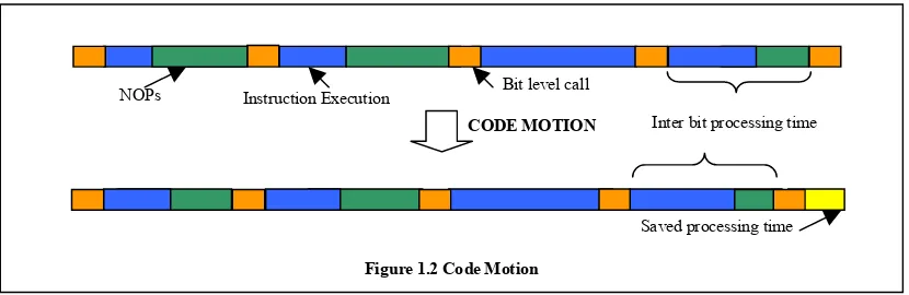
The question is how we can improve this scenario to utilize the time in which the NOPs are inserted. We propose to perform code motions within the message level function to utilize the NOP execution times. This thesis describes how code motion is performed from a inter bit path with the maximum inter bit processing time to inter bit paths with lower inter bit processing time. This process will reduce the maximum inter bit processing time and thereby increase the idle time available at the bit level layer to improve the efficiency of the processor. This concept is illustrated in figure 1.2.

Much of the algorithm concepts and ideas have been derived from traditional syntactic code motion by Knuth et. al. Their papers on dead code elimination (DCE) and partial redundancy elimination (PRE), [KRS 1] [KRS 2] [KRS 3] [KRS 4], have helped us in understanding the relationships that exist among the variables of a given program and the concepts of code hoisting and code sinking. These algorithms have also helped us in understanding the intricacies of data flow analysis and helped in our own conception of a new form of data flow analysis. We have derived a new algorithm based on these concepts wherein instructions themselves are moved rather than the computations in expressions, as done by these authors. Furthermore our algorithm works with registers as opposed to variables in DCE and PRE algorithms

Figure 1.1 Inter-Bit processing time distribution

Saved processing time CODE MOTION

NOPs _{Instruction Execution} Bit level call

Figure 1.2 Code Motion

C h a p t e r 2

BACKGROUND

2.1 Software Thread Integration

STI [DEA 1] is a compiler technology, which interleaves multiple assembly language threads at a fine-grain level. The resulting thread offers low-cost concurrency, but still executes on a generic processor without fast context switches. STI can be used for hardware to software migration (HSM). HSM is the process of moving functions from dedicated hardware components to real-time software. HSM helps to improve system cost, size, weight, power, function availability, time to market, and field upgrades. The main targets of HSM are embedded systems which cannot afford the luxury of a high performance microprocessor yet require fine-grain thread concurrency.

Performing this type of integration is tricky. Static timing analysis is performed on the control dependence graph generated for both the threads. This timing analysis gives us information about how early or how late an instruction would be executed when the threads are run and also how long the instructions take to complete the execution. This type of information helps in identifying insertion places in the host thread, where instructions from the guest thread can be placed so that the real time requirements of the guest thread is properly met. CDGs facilitate easier implementation of static timing analysis and provide excellent support for determining the insertion points that meet the real time constraints in the host thread and the subsequent placement of the guest code in those locations. Register reallocation techniques are also employed to enable sharing of the processor’s register set by the two threads, without any conflicts.

STI is extremely valuable for recovering idle time from real-time guest threads performing low-level (e.g. MAC and data link layer) network communication and video refresh functions. Other applications with significant fine-grain idle time can benefit from STI as well. An example of an application in which STI has been implemented is given in [DEA 2] in which high temperature (185-225 C) CAN network interface is implemented in software and integrated with buffer management code for the CAN protocol. This system has been built and tested at up to 225 C. A special compiler called thrint has been developed for this purpose. Thrint is a post-pass (back-end) compiler which reads assembly code, performs control-flow, data-flow and static timing analysis, and integrates threads.

2.2 STI for BBCP

STI concepts were employed in [KUM 1] for improving the performance of BBC protocols used in embedded networks. Examples of embedded protocols are J1850, CAN, 1553, etc. These protocols are extensively used for communication among embedded devices connected in a network. An example of such a network would be a car in which the various parts of the car are connected together in a network for proper functioning of the car.

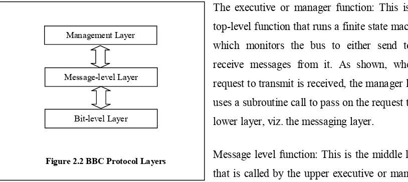
For STI in BBCP, the protocol functions are implemented in three layers. This scheme is illustrated in figure 2.2. Figure 2.3 gives an example of such a three layer stack using a send function. The three layers are explained below:

The executive or manager function: This is the top-level function that runs a finite state machine which monitors the bus to either send to or receive messages from it. As shown, when a request to transmit is received, the manager layer uses a subroutine call to pass on the request to its lower layer, viz. the messaging layer.

Message level function: This is the middle layer that is called by the upper executive or manager layer. This consists of functions that handle messages, such as send_message function or receive_message function. This function performs all the encoding/decoding schemes of the protocol and passes the messages to the corresponding layers. In addition to these, depending on the protocol, the messaging layer may also be responsible for calculating the CRC (when sufficient time does not exist in bit level layer to perform these functions) and checking whether the received CRC is same as the calculated CRC.

Bit level function: This is the bottom-most layer. This layer takes care of sending or receiving bits to or from the bus. The function that runs at this layer is a real time function, as it has to meet the timing requirements of sending and receiving bits at the appropriate instant. This function is invoked by the message level layer. For example, the send message function invokes the send bit function at this layer. The bit level function may also be responsible for additional functions such as bit stuffing, CRC/parity generation/check

The three layers are implemented independently. As can be seen from figure 2.3, the bit level function has coarse grain idle time, which would be wasted by busy wait or by interrupt processing depending of which method is used for meeting the real time constraints. To recover these fine-grained idle times and use them to perform other tasks by the processor, the bit level function is integrated with the upper management level function. A concept called Cocall was introduced to switch between these two threads.

Management Layer

Message-level Layer

Bit-level Layer

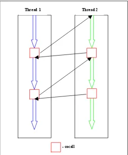
Cocalls are similar to subroutine calls. A co-call operation is used to transfer control between two processes. A co-call is effectively a call and return instruction combined into one operation. From the point of view of the process executing the co-call, the operation is equivalent to a procedure call and from the point of view of the process being called; the co-call operation is equivalent to a return operation.

Thread 1 Thread 2

Thus, unlike subroutines, when the second process cocalls the first, control resumes not at the beginning of the first process, but immediately after the co-call operation. If the two processes execute a sequence of mutual co-calls, control will transfer between the two processes as shown in figure 2.4

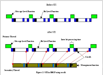
Asynchronous Software Thread Integration (ASTI) is performed to remove the time critical code from the bit-level function to create a longer idle time for a secondary thread to run. The secondary thread is modified such that it cocalls back to the primary thread just before the end of the enlarged idle time. The code removed from the primary thread is integrated with the secondary thread so that it is executed at the correct times. Both the threads are then padded with NOPs to eliminate jitter. The bit-level functions are modified so that they run for a fixed amount of time. The message level functions are first padded to reduce jitter and then padded to make the calls to the bit level functions occur at a fixed frequency. The secondary thread which contains the management function is padded to remove jitter. Thus the resulting threads are as shown in figure 2.5. More details about the various stages of integration is given in [KSA 1]

Inter bit processing time

Management function Cocalls

Message Level Function Bit Level Function

Figure 2.5 STI in BBCP using cocalls

Before STI

After STI

Message Level Function Bit Level Function

C h a p t e r 3

RELEVANT RESEARCH

3.1 Code Motion

Code motion is a relatively old concept and significant research has been done in the field. This section gives a brief account of the various research results for code motion. Traditionally code motion has been aimed at improving generic programs which run in generic processors. These types of code motion can be classified as “higher-level” code motion. The intent in this type of code motion is to move instructions that are redundant (partial redundancy elimination) or dead (dead code elimination) when traversing the program along one of its flow paths. So the net effect is to move code so that the average execution time of the program can be reduces. At the other end of this code motion spectrum is the “lower-level” (“machine-level”) code motion. Algorithms performing “lower-level” code motion work on the machine or assembly level of the programs. These programs try to move high-delay instructions such as loads and stores to various parts of the program to improve the run-times of a program. These types of algorithms are machine specific and can vary from architecture to architecture. Significant research has been carried out in this field as well.

3.2 Higher-Level Code Motion

Syntactic code motion relates instructions (assignments or expressions) based on the syntax of the instruction i.e., how the instruction appears in the program. It does not consider the relationships among the values stored in the variables used in the instruction or the result of an instruction.

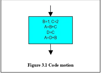
Semantic code motion relates instructions based on the values of the variables involved in the instruction and the result of the instruction. In figure 3.1, the value of A on the second and the fourth line is the same (value is 3), but the syntax is different in the second and the fourth line. Thus whereas syntactic code motion might find the fourth line of code unnecessary and remove it, syntactic code motion fails to identify that the two lines of code do the same task and will not perform any code motion. Since their syntax is different syntactic code motion treats them as two separate instructions.

3.3. Syntactic Code Motion

Syntactic code motion has been extensively researched by Knoop, Ruthing and Steffen. They have published various algorithms for syntactic code motion in [KRS 1], [KRS 2], [KRS 3] and [KRS 4]. This section describes the code motion and the algorithms briefly.

3.3.1 Critical Edges

A critical edge is an edge in the flow-graph from a block with multiple successors to a block with multiple predecessors. Critical edges pose a problem for many code motion algorithms, as it makes it difficult to move an assignment or expression to the middle of the edge. For example figure

AB

C

B

A

Figure 4.2 Critical Edge Splitting

A

B

C

B

A

Dummy

B=1, C=2 A=B+C

D=C A=D+B

3.2(A) shows a critical edge named AB. To overcome this problem the authors propose a process of edge splitting, which is the insertion of a block (dummy block) in the middle of the critical edge. This breaks the critical edge and enables movement of code into the dummy node.

3.3.2 Partial Dead Code Elimination

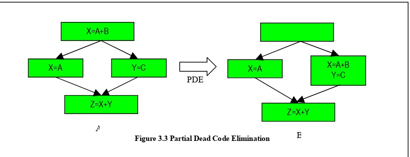
In [KRS 1], Knoop, Ruthing and Steffen propose an algorithm that eliminates partial dead code as much as possible without modifying the program structure or affecting the other parts of the program. An assignment is said to be partially dead if some but not all the paths from the assignment to the exit of the program contain a use of the variable that is being assigned. An example is shown in figure 3.3. In code A, the assignment X=A+B is said to be partially dead along the path through the left side of the branch, as X is redefined in X=A along that branch and there is no use of the value stored in A in between the two definitions. But it is not dead along the right side of the branch as the value of X assigned before the branch is used in the statement Z=X+Y. So after applying partial dead code elimination the new flow-graph as shown in B, eliminates the need for performing the assignment X=A+B, when traversing along the left side of the branch thereby reducing the runtime along that branch.

The proposed algorithm consists of two separate steps:

Faint Assignment Elimination – In this step faint variables from the program are identified. A variable is said to be faint at a point in a flow graph if, on every path from that point to the exit of the program, any use of the variable is either preceded by a redefinition of the variable, or occurs within an assignment to a variable which is also faint. This step starts by assuming that all the

X=A+B

X=A Y=C

Z=X+Y

Figure 3.3 Partial Dead Code Elimination

X=A X=A+B

Y=C

Z=X+Y PDE

A

variables are faint everywhere, except arguments of a procedure call and return variables. Then, iterative backward analysis is performed as follows:

N-FAINTi(x) denotes whether the variable x is faint at the beginning of an instruction or

assignment i.X-FAINTi(x) denotes whether the variable x is faint at the end of an instruction or

assignment i.

The faint variable analysis is given as

N-FAINTi(x) = ~RELV-USEDi(x) Λ (XFAINTi(x) V MODi(x))

Λ (XFAINTi(lhsi) V ~ASSIGN-USED i(x))

X-FAINTi(x) = Π j ε succ(i) N-FAINTj(x)

The predicates used are

RELV-USEDi(x) – x is a right-hand side variable of the relevant instruction i. (variables occur only

on the right hand side of relevant instructions).

MODi(x) – x is the left-hand side variable of the instruction i.

ASSIGN-USEDi(x) – x is the right-hand side variable of the assignment statement i.

After computing the greatest solution for the above set of equations for the variables corresponding program transformations are performed.

Assignment Sinking – Assignment sinking is the motion of assignments within a flow-graph in the direction of program execution. Here a set of equations are computed for each sinkable statement and delay ability analysis is performed which determines how far an instruction can be sunk along the program flow.

3.3.3 Partial Redundancy Elimination

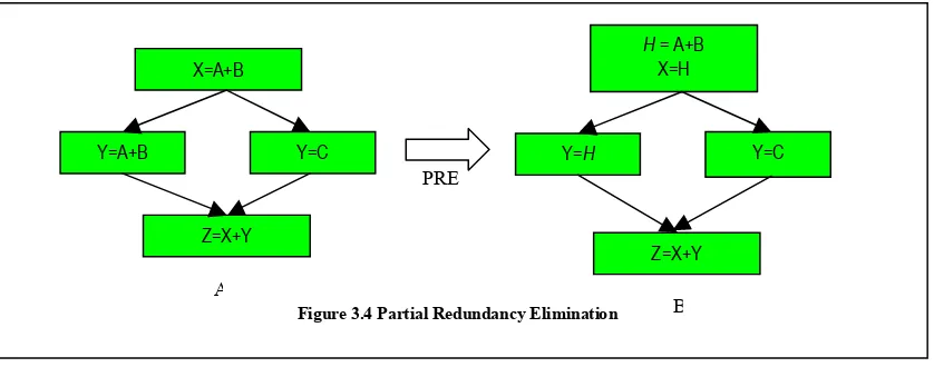
the two expressions. Thus the expression A+B is said to be partially redundant. Note that the expression is redundant only along the right side of the branch

and not along the left side of the branch. Applying PRE we can store the value of the expression A+B in a temporary variable H and use it in the two assignments as shown in figure 3.4(B).

The proposed algorithm determines D-SAFE points for each computation and determines how far a computation can be hoisted. Hoisting the computation as shown in the example removes partially redundant computations from the program. For a computation t, the D-SAFE at the various nodes (code blocks) of the program is computed using the greatest solution of the following equation system.

D-SAFE(n) = false if n=EXIT NODE Used(n) V

Transp(n) Λ Π m ε succ(n) D-SAFE(m) otherwise

D-SAFE can be defined as follows: a node n is n-down-safe if and only if D-SAFE(n) holds. Then the earliestness of the nodes are computed using the following system of equations:

EARLIEST(n) = true if n=s _Σm ε pred(n) ( ~Transp(m) V

~D-SAFE(m) Λ EARLIEST(m)) otherwise A node n is n-earliest if and only if EARLIEST(n) holds.

X=A+B

Y=A+B Y=C

Z=X+Y

Figure 3.4 Partial Redundancy Elimination

H= A+B X=H

Y=H Y=C

Z=X+Y PRE

A

Using the D-SAFE and the EARLIEST values for the nodes computed, the Safe-Earliest Transformation can be performed as follows:

• Introduce a new auxiliary variable h for the term t.

• Insert at the entry of every node n satisfying D-SAFE and EARLIEST the assignment h:=t. • Replace every original computation of t in the program by h.

Whenever D-SAFE(n) holds, there is a node m on every path p from start to n satisfying D-SAFE(m) and EARLIEST(m) such that no operand of t is modified between m and n. Thus all replacements of the above algorithms are correct. The authors also propose some special features to remove unnecessary code motion which does not improve the run-time of the program. This is called the lazy code motion algorithm.

In [KRS 4], the same authors proposed a similar algorithm with aggressive code motion. In the above lazy code motion algorithm the expressions are moved up only as far enough to perform code optimization. In the aggressive code motion algorithm, code motion is performed on every expression, resulting in the hoisting of the expressions as far up as possible. This had the disadvantage of increase in register pressure due to intermingling of expressions, which resulted in increase in the number of live variables.

A more structured approach for partial redundancy elimination is given in [CCK 1]. The authors propose an algorithm for partial redundancy elimination, which achieves optimal code motion similar to “lazy-code”. The algorithm is based on SSA for of a program and tries to eliminate the iterative data flow analysis and bit vectors in its solution. In [BGS 1], a new profile based redundancy elimination algorithm is proposed in which cost of code growth is weighed against the benefit of code motion to justify code motion. This algorithm is proposed for code motion in programs meant for embedded real-time applications.

In [STE 1], the author suggests a combined algorithm for code hoisting and code sinking. Code hoisting and code sinking work in opposite directions of the program flow and consequently when the two are applied together to a program, it would result in the two algorithms enabling each other after each pass of the algorithm. The paper hypothesizes the following points about the combined approach

2) Iterate the following until the code stabilizes: a) Redundant assignment elimination. b) Faint assignment elimination. c) Assignment hoisting.

3) Iterate the following until the code stabilizes a) Faint assignment elimination.

b) Redundant assignment elimination. c) Assignment hoisting.

4) Apply a backwards copy propagation algorithm to eliminate unnecessary temporary variables (h).

3.4 Semantic Code Motion

Semantic code motion extends syntactic code motion algorithms to perform code motion of expression that evaluate to the same value. Semantic code motion performs better optimization compared to syntactic code motion as explained earlier. Value numbering has been one of the major approaches in performing semantic code motion. The primary objective of value numbering is to assign an identification number called value number to each value that is computed in a program in such a way that two values have the same number if the algorithm can prove that they are equal under all possible values of inputs and control flow. This section describes the research results in the field of semantic code motion.

Semantic code motion is generally based on Static Single Assignment (SSA) forms of programs. In the SSA, each variable name in the program occurs only once on the left hand side of the flow-graph. This makes the relationship between the definition of a variable and its use in the program more explicit. When more than one value for a variable is possible at the beginning of a block, depending on the branch along which control enters the beginning of the block, φ functions are used to determine which value of the variable is used in the block. A detailed description of SSA form is given in [BHS 1]. In [CFR 1], an efficient algorithm for obtaining the minimal SSA form of the flow-graph is presented.

3.4.1 Hash-Based Value Numbering

number if they are provably equal. This algorithm though works only inside code blocks and does not expand over the entire program.

In [BCS 1], the authors extended the hash based algorithm of [COC 1], to perform hash-based value numbering over and entire program by using a single hash table for all the basic blocks. This method proceeds by traversing the control flow graph (CFG) of a given program in reverse post-order and process the φ functions and instructions in each block. For processing the φ functions in a block, the algorithm checks to see if there are any incoming back edges. If there is back-edge and the φ function refers a value coming through the back edge, the parameter of the φ function may not have a value number assigned to it. In this case, the compiler assigns a unique value number to the incoming parameter. If there are no back-edge flows into the block, the reverse post-order traversal guarantees that all the _φ function parameters have been assigned value numbers. Thus each block of the program is analyzed completely. When processing the φ functions, the algorithm overwrites the operands with their value numbers, simplifies algebraic expressions and performs code motion on the resulting expression. If an expression similar to the simplified one is found in the hash table, the result is overwritten with the same value number of the expression. Otherwise, the expression is added into the hash table and the algorithm proceeds. But this algorithm cannot handle values that flow through back edges and does not work well with programs containing loops.

3.4.2. Value Partitioning

3.4.3 SCC-Based Value Numbering

In [COO 1], an algorithm that works in conjunction with Trajan’s algorithm [TAR 1] for finding strongly connected components (SCCs). Tarjan in his algorithm uses a stack to determine which nodes are in the same SCC. Nodes which are contained in a cycle are popped out of the stack together, whereas nodes that do not belong to any cycle are popped out of the stack singly. This concept of SCC was used in [COO 1] to identify nodes in which there is a flow of data through the back-edges. When a single node is popped from the stack, value numbers would already have been assigned to the operands of the corresponding expression and hence a value number can be assigned to the expression easily. When a collection of nodes representing an SCC is popped, we would have assigned value numbers to any operands outside the SCC. The nodes of the SCC need to be handled differently, while computing their value numbers. The value numbers for the nodes in the SCC are assigned by iterating in the reverse post-order. Initially the value for each member of the SCC is assumed to be some unknown value. The unknown value indicates that the value number for that member has not been computed yet. Then optimistic assumptions are made in an iterative process and the values are stored in an optimistic table. Then when the iterative process stabilizes, entries are added to the main valid table. Note that for single nodes values are directly added to the valid table.

The reverse post order algorithm proposed by the authors in this paper is as follows 1) Initialize VN[x] = T for each SSA based name x.

2) Repeat the following:

a) Iterate through the blocks in the reverse post-order.

i) Iterate forward through the definitions α in the current block. ιι) Set VN[α] = lookup([α]).

b) Remove all entries from the hash table. 3) Until no changes to NV[] occurs.

In [COO 2], Cooper and Simpson propose a value-driven code motion algorithm which performs code motion to eliminate computations of redundant values. This is in contrast to the syntactic code motion which performs code motion to eliminate redundant assignments. Value driven redundancy analysis is performed over a domain of values instead of assignment. The predicates used in his algorithm are

• EXECUTED-LOCAL(b) – this is a set of values computed by assignments in the block b. • REDUNDANT-IN(b) – this set contains values which have already been computed along

every execution path from start to the beginning of the block b.

• REDUNDANT-OUT(b) – this set contains values which have already been computed along every execution path from start to the end of the block b.

For local analysis is performed to determine the EXECUTED-LOCAL set for each block of the program. Then REDUNDANT-IN and REDUNDANT-OUT which are defined recursively as follows are computed for each block:

REDUNDANT-IN(b) = {} ,for b = start Π p ε pred(b) REDUNDANT-OUT(m) ,otherwise

REDUNDANT-OUT(b) = EXECUTED-LOCAL(b) U REDUNDANT-IN(b)

The above analysis is applied to the program from the start node to the end node in the forward direction, until the values of the predicates REDUNDANT-IN(b) and REDUNDANT-OUT(b) stabilize. This method is called iterative forward analysis. The actual transformation is performed as follows:

• Scan through each block of the program in the forward direction. • Update the contents of REDUNDANT-IN(b) after each instruction.

C h a p t e r 4

CONCEPTS

4.1 Control Flow Graphs (CFGs)

Control flow graphs are graphical representations of the flow/sequence of execution of a program. We use control flow graphs as a first step towards obtaining the control dependence graphs.

Definition 4.1: A control flow graph is a directed graph G augmented with a unique entry node START and a unique exit node STOP such that each node in the graph has at most two successors.

We assume that nodes with two successors have attributes “T” (true) and “F” (false) associated with the outgoing edges in the usual way. We further assume that for any node N in G there exists a path from START to N and a path from N to STOP.

4.2 Control Dependence Graphs (CDGs)

Control dependence graphs are also graphical representation of programs. But CDGs represent the dependence relationship that exists between instructions in the program. For example, an instruction i, present inside an if instruction is dependent on the if instruction. Ferrante et. al. define CDGs as follows in [FER 1]

Definition 4.2:Let G be a control flow graph. Let X and Y be nodes in G. Y is control dependent on X iff

1. There exists a directed path P from X to Y with any ∈ in P (excluding X and Y) post-dominated by Y and

2. X is not post-dominated by Y.

Definition 4.3: A sequence of basic blocks is said to be structured iff the CDG generated has an hierarchical structure. i.e., if a ! b (a depends on b) and a! c, then either b! c or c!b is true (a, b and c are different basic blocks).

This type of CDG is chosen for STI because of the following reasons

• The timing analysis can be performed correctly without ambiguity using the CDG. • Accurate timing intervals can be identified in the code

• Insertion of guest code into the host CDG can be done accurately to meet the timing constraints of the guest code

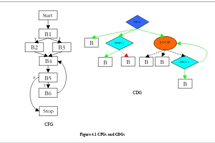
A simple example for a CFG and its corresponding CDG is shown in figure 4.1

Every code block in the CFG is represented as CODE node (square shaped nodes) in the CDG. The node B2 is represented as a CODE node in the CFG. When a basic block has a conditional branch at its end, the conditional instruction is placed in a PRED node (diamond shaped nodes) in the CDG. The code block B1 has a conditional branch at its end. This instruction is represented as the PRED node PRED 1. Loops are represented using a LOOP node (ellipse shaped node) as shown in figure. The loop involving the nodes B4, B5 and B6 is represented as the node LOOP 1.

T F

F T

Start

B1

B2

B3

B4

B5

B6

Stop

PROC

B

B

B

B

B

B

CFG

CDG

The arrows in the CDG point to the dependents of each node. The green or line arrow indicates a dependency based on TRUE result of the conditional instruction (Example – arrow from PRED 1 to B2). The red of dotted arrow indicates a dependency based on FALSE result of the conditional instruction (Example – arrow from PRED 1 to B3). The black or dashed arrows indicate a straightforward unconditional relation (Example – arrow from LOOP to B4). This type of arrow is used only for unconditional children of a LOOP node. In other words this arrow links nodes which execute at least once in a loop to the LOOP node. A detailed explanation fo the CDG format is given in [DEA 1].

4.3 Labels

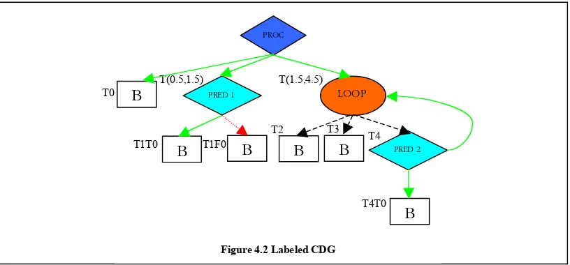
Labels were introduced in [NEW 1]. The node labeling scheme proposed can be used for assigning labels to each node in a CDG. This labeling scheme helps to determine the relative positions of the nodes by just comparing their labels. This also facilitates computation of reachability, dominance and control dependence relationships, as well as node-to-node traversals. Without the labeling scheme, the evaluation of the above relations would require traversing the entire tree from node-to-node.

We use labels in our algorithms for the same reasons of improving the efficiency in obtaining the relationships between the various nodes in the CDG. Each node is assigned a label in this scheme. Each label consists of an array of cells. The number of cells a label contains depends on the depth

T4T0 T(1.5,4.5)

T3 _T4

T2 T1F0

T1T0 T(0.5,1.5) T0

PROC

B

B

B

B

B

B

of the node in the CDG. So if a node is at a depth of n from the root of the CDG it will contain n cells. For the CDG constructed in the previous section, the labeled CDG is shown in figure 4.2. The ith _{cell of a label corresponds to the position of the node in the CDG with respect to the}

conditional node at level i. Each cell in the label has three fields. Thefirst field specifies which side

of the conditional the node is present. There can be two values either T for true or F for false. The second field contains the section number. The section number is the relative distance of the node from the first node in the same side of the conditional. So the values of the section number start from 0. When new nodes are inserted in between existing nodes in the CDG section numbers with non-integer values can be used to avoid renaming all the node labels. The third field contains a pointer to the conditional node at the level indicated by the cell i.e., the ith _{conditional in the}

hierarchy for the ith _cell.

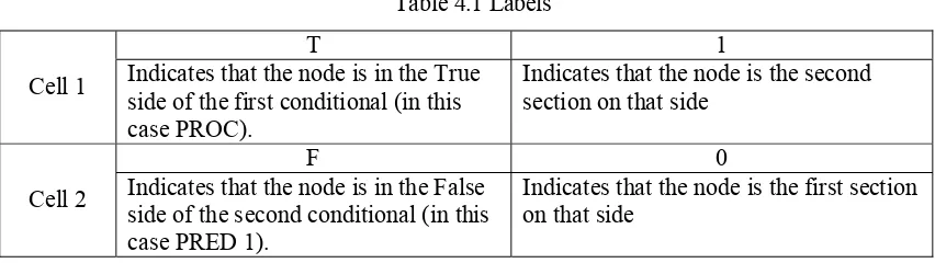
For example, consider the node B3 in figure 4.3. Its label (T1 F0) can be separated into 2 cells and its position information can be extracted as follows.

Table 4.1 Labels

T 1 Cell 1 Indicates that the node is in the True

side of the first conditional (in this case PROC).

Indicates that the node is the second section on that side

F 0 Cell 2 Indicates that the node is in the False

side of the second conditional (in this case PRED 1).

Indicates that the node is the first section on that side

children to the LOOP node. For example, the PRED node PRED1 has a range of T0.5 to T1.5. Its child nodes have a section number of T1 for the corresponding level of hierarchy. Similarly LOOP node LOOP1 has a range of T1.5 to T4.5. It has three immediate children and they each have the section number T2, T3 and T4 from left to right as shown. The main PROC node does not have any label and is at the top level of the hierarchy.

In [NEW 1], the following list of properties is provided for the labels.

• Use of labels – represents the location within the program structure locally, which facilitates evaluation of relations, traversal and code motion, especially along multiple paths

• Every label is unique – no ambiguity exists among labeled nodes, guarantees that nodes can always be inserted without changing any other labels.

• Each cell of a label has a pointer to a CDG node – facilitates the assignment of control dependences and arcs from group nodes during CDG construction.

• Each nodes has a label for each aggregate conditional path that it is on – facilitates the computation of reach ability and domination, makes certain path properties more easily provable.

• Beginning and ending labels – limits the scope of CDG traversal in order to assign labels to newly-inserted region nodes; aids in upwards and downward CDG traversal.

In the case of unstructured code, there is a possibility that a node may have two labels. This is due to the fact that a single node may be the child of two different nodes in the CDG caused by the unstructured nature of the code which allows a node to be dependent on two different nodes. For our case this will not occur as we deal only with structured code. In structured code, each node is dependent on only one other node and hence each node has only one parent. [NEW 1] also describes some algorithms can be used effectively for determining the location details and relative spacing of nodes in a CDG. We will present the details of these methods and how they are used in the algorithm later.

4.4 Movable and Non-movable statements

under consideration. So while designing the algorithm for optimizing the inter-bit processing time, the architecture of the processor is also considered to some extent.

A major difference in low level code motion and high level code motion is the fact that some instructions in the low level code motion cannot be moved while preserving the semantic correctness of the program. We classify these types of instructions as non movable instructions. Our algorithm des not perform any action on these instructions and no data flow analyses are performed either. When a non movable instruction occurs it is just skipped and the analysis carries on for the next instruction (either in the up direction or the down direction).

We have analyzed the different types of assembly instructions and have arrived at the following list of non-movable instructions.

1. Skip instructions & Branch instructions – (sbrc, jmp, jnez) These instructions decide the flow of control along the program. Moving these instructions would alter the control flow. 2. Conditional instructions – (cmp, tst) Any instruction which defines the flag, which is used

by a conditional branch instruction is the conditional instruction. Control flow of the program is decided by these instructions. Moving this type of instructions would affect the control structure of the program.

3. Pointer instructions – (ld, st) These are indirect memory addressing instructions. These instructions cannot be moved as they define or use values which are stored in memory locations, the address of which is stored in registers. Further these instructions also affect the way in which other memory based instructions are moved. As the memory locations addressed by these instructions are not predictable, other memory based instructions could not be moved past these instructions.

The distribution of the non-movable instructions is shown in figure 4.4 0 10 20 30 40 50 60 70 80 N o . of I n st ru ct ions

CAN Send CAN Recv 1553 Send 1553 Recv

Different Types of Non-movable Instructions

Pointer Store Pointer Load Branch and associated Instructions Flag Register

We analyzed several different programs and obtained the graph shown in figure 4.3. From the figure we can see that on average; two thirds of the instructions are movable in a program. As the percentage of movable instructions increases, we can obtain a better optimization.

0 50 100 150 200 250 No . o f In st ru ct io n s

CAN Send CAN Recv 1553 Send 1553 Recv Average Instruction Types

Movable instructions Non-movable Instructions

Figure 4.3 Movable Vs Non-movable instructions

From the figures we can observe the following.

• The number of branch and conditional instructions is in general proportional to the number of instructions present in the program.

• The number of flag affected instructions is very less. In most cases it is a very small negligible percentage of the total number of instructions.

C h a p t e r 5

PRELIMINARIES

5.1 Why Code Motion is done at assembly level?

Since the thread integration is performed at a lower assembly level, the timing analysis takes place at the assembly level as well. Another reason for performing timing analysis at the assembly level is the accuracy of the timing analysis as the assembly instruction timings can be predicted accurately. The same would not be possible at a higher language level.

Assembly level is the most appropriate level to perform code motion. As mentioned in chapter 4 most of the relevant research has been either in the higher level or lower level. In the higher level code motion, code movement is performed for expressions and assignments which are redundant or dead at places. The lower level code motion involves the movement of the machine level code to exploit the microprocessor design underneath for extracting some efficiency. Our code motion is different from these two approaches. Our code motion tries to move assignment and other register manipulation instructions at the assembly level to improve the inter-bit processing times that exist when code integration is performed for Bit-Banged communication protocols. This is not a generalized code optimization technique. But rather this is a software thread integration specific code optimization algorithm. This thesis concentrates on explaining the algorithm as we have implemented it for the AVR-RISC processors. But in general this algorithm can be expanded to any RISC processor with some changes in the timing analysis and classification of the instructions that can be moved.

5.2 Why CDGs are used?

the concept of labels (explained in chapter 3), node identification and search becomes very easy and efficient while using a CDG. Thus we have designed our algorithm to work on the CDG representation of the program. Though for clarity purposes and easy understanding we explain the algorithm in detail using CFGs and explain its implementation on the CDG representation.

5.3 Inter-Bit Timing Analysis

In order to perform code optimization and code motion, we need to determine from which paths code needs to be moved. Code has to be moved from paths that take a longer time to run, to paths which take shorter time to run. In order to identify this we need to perform timing analysis of all the inter-bit paths that exist in the program.

In this section we present a simple yet efficient timing analysis algorithm which we use to identify the run times of the different inter-bit paths that exist in the program. We present a brief discussion of the algorithm here.

Definition 5.1: An inter-bit path is defined as the set of nodes (CODE/LOOP/PRED) between subsequent CALL nodes that can occur in the CDG of a program. By subsequent we mean the subsequence during the run-time of the program.

There may be many inter-bit paths for a given CDG of a program. Some inter-bit paths are traversed many times when the program is executed and some may not be traversed at all. But all the inter-bit paths that are possible have to be taken into account when timing analysis is performed.

Timing analysis gets a little complicated for inter-bit paths as there can be numerous possible ways in which a program flow can take place. For example for the simple CDG shown in the figure 5.1, the number of inter-bit paths possible is 6.

The various paths are

C1 ! B1 ! P1 ! B3! B4! B5 ! C3 C2 ! B6 ! B4 ! B5 ! C2

C2 ! B6 ! B4 ! B5 ! C3

To simplify the task we do not explore the various paths possible for PRED and LOOP nodes which do not have any CALL nodes below them. In our example we have the PRED node P1 which has two children B2 and B3, but does not have any CALL node. But instead of considering the two possible paths that are available at the PRED node (along either branch), we take just the PRED node as a single node with a finite run-time. This run-time would be the greatest run-time of the branches of the PRED node

In the case of LOOP nodes which do not have any CALL nodes below them, we determine the run-time of the entire LOOP node by using data-flow analysis or directions from the user about the number of times each loop executes. The user can provide this information through the ID file in our implementation (thrint). Based on the number of times a particular loop runs we can calculate its run-time by using simple calculations. Thus after this simplification each PRED or LOOP node that does not have any CALL node below it, would be simplified as a single node with finite run-time.

For our example the simplification reduces the number of paths to 4 and the paths are C1 ! B1 ! P1 ! B4 ! B5 ! C3

C1 ! B1 ! P1 ! B4 ! B5 ! C2 C2 ! B6 ! B4 ! B5 ! C2

C1

B5

C2

P2

C3

B2

P1

B1

B3

B4

C2 ! B6 ! B4 ! B5 ! C3

5.3.1 Algorithm details

LivePaths – Set that contains the list of paths for which the run-time is being calculated.

AppendNew(pathlist,i) – Appends a new path to pathlist. The new path is a copy of the path number i in pathlist.

AddDuration(pathlist,dur) – Adds dur cycles to the duration of all the paths in pathlist. RemovePath(pathlist,i) – Removes the path i from pathlist.

Type(node) – Gives the type of node.

NextChild(node,tv) – Gives the next child of node with truth value tv.

LoopReturn(node) – Is true, if node is the LOOP node and is already visited or is being visited. HasCALL(node) – Is true, if node has a CALL node as one of its descendants

Duration(node) – Duration of node in cycles

SDuration(node) – Duration of the entire subgraph with node as the root IsLCP(node) – Is true, if node is a loop closing PRED

node – current node (the algorithm is started with node=start)

createnew – indicates whether new paths have to be created (initially false)

5.3.2 Algorithm

The algorithm for computing the various inter-bit paths is as follows Inter-Bit Analysis(node,createnew)

if Type(node) = PROC do

next= nextchild(node,TV_T)

while next do

Inter-BitAnalysis(next) next=nextchild(node,TV_T)

else if createnew

for every path p in LivePaths

AppendNew(LivePaths,p) if LoopReturn(node)

AddDuration(LivePaths,Duration(node)) If Type(node)=LOOP

If not HasCALL(node)

AddDuration(LivePaths,SDuration(node)) else

next=nextchild(node,TV_T)

while next do

Inter-BitAnalysis(next) next=nextchild(node,TV_T)

while next do

Inter-BitAnalysis(next) next=nextchild(node,TV_T)

if Type(node)=PRED and IsLCP(node) if node called first time

If not HasCALL(node)

AddDuration(LivePaths,SDuration(node)) Else

AddDuration(LivePaths,Duration(node)) tv=truth value of first child of node

next=nextchild(node,tv)

Inter-BitAnalysis(next,true) next=nextchild(node,tv)

while next do

Inter-BitAnalysis(next)

next=nextchild(node,tv)

else

AddDuration(LivePaths,Duration(node)) if Type(node)=PRED

if not HasCALL(node)

AddDuration(LivePaths,SDuration(node)) Else

AddDuration(LivePaths,Duration(node)) tv=truth value of first child of node

next=nextchild(node,TV_T)

Inter-BitAnalysis(next,true) next=nextchild(node,tv)

while next do

Inter-BitAnalysis(next)

while next do

Inter-BitAnalysis(next)

next=nextchild(node,TV_F)

if Type(node)=CALL

for every path p in LivePaths ending in node Remove(LivePaths,p)

5.4 Code Motion Algorithm Specifics

5.4.1 Predicates Used

Two predicates IS-DEFINED(i,r) and IS-USED(i,r) are used in the algorithm

IS-DEFINED(i,r) – indicates whether the instruction i defines the value in the register r. In case r

denotes a register set, this indicates whether instruction i, defines at least one of the registers in the register set r.

IS-USED(i,r) – indicates whether the instruction i uses the value in the register r. In case r denotes a register set, this indicates whether instruction i, uses at least one of the registers in the register set

r.

Two sets USED(i) and DEFINED (i) are used

USED(i) – holds the registers whose values are used by the instruction i. DEFINED (i) – holds the registers whose values are defined by the instruction i.

The D-SAFE and U-SAFE predicates (to be described later) can hold any of the four values R_FALSE, R_TRUE, C_FALSE and C_TRUE. These four values are defined as follows:

1. NONE: Indicates that the predicate has not yet been computed.

The “C_” prefixed values are used for nodes, for which it is exactly not known at the time, whether code motion could or could not be performed. These values are also used for nodes into which we would not be moving our code in general for the current data flow analysis. For example when we are trying to perform a code hoist from a node A and another node B always follows A, we would not be considering B to move the code from A. these values are also used when processing loop nodes as some complexity is involved when performing data-flow analysis for them. We will explain more about this in later chapters. The “R_” prefixed values are used for nodes which can be potentially candidates for code motion, as we want to know exactly whether code can be moved or cannot be moved to these nodes.

The operations for these predicates are similar to the Boolean operations performed in other code motion algorithms, though slightly different. We define here the operations that can be performed using these predicate values and the results of the operations. The operations are the same as the Boolean operation when

• The operand values have only C prefixes or no prefixes • The operand values have only R prefixes or no prefixes

The result in the above two cases can be obtained by removing the prefixes from the operand values and performing normal Boolean operations. The result is then prefixed with the prefix of the operands.

AND operation: The AND operation is similar to the Boolean AND operation. If the operands have a mix of both C prefixed and R prefixed values, the AND operation is defined as follows:

Table 5.1 AND Operation

A B A AND B

OR operation: The OR operation is similar to the Boolean OR operation. If the operands have a mix of both C prefixed and R prefixed values, the OR operation is defined as follows:

Table 5.3 OR Operation

A B A OR B

R_TRUE C_TRUE R_TRUE R_TRUE C_FALSE R_TRUE R_FALSE C_TRUE R_TRUE R_FALSE C_FALSE R_FALSE

For CFGs, start and end denote the start node and end node respectively unless specified otherwise. The start node does not have any predecessors and the end node does not have any successors. The programs as already mentioned, are assumed to be structured code and there should not exist any multiple dependencies.

Instr(n) denotes the set of instructions in the node n. PrevInstr(i,n) denotes the set of all the instructions that occur before the instruction i, in the node n.

5.4.2 Labels

Labels assumed to have been assigned to each node in the CDG. The functions that are provided by the labels are:

Before(node1,node2) : returns true if node2 precedes node1 in the control flow sequence. After(node1,node2) : returns true if node2 follows node1 in the control flow sequence. Locate(labels): returns the node n with label labels if present in the CDG

5.4.3 Dummy nodes

Dummy nodes are inserted into the CDG at various places. These are CODE nodes with no instructions. Dummy nodes help in simplifying the data flow analysis of the CDG and also act as place holders for code placement during code motion.

Dummy nodes are inserted at the following places in the CDG:

For PROC node: For PROC nodes, a single dummy node is inserted as the last child of the PROC node. This node acts as a place holder while moving instructions down. This node is names as proc_EN, where proc is the name of the PROC node and EN stands for END.

For CALL node: For CALL nodes, dummy nodes are inserted before and after each CALL node. These nodes mainly serve are place holders during code placement to hold instruction that are moved. These nodes are names name_CP and name_CS, where name is the name of the CALL node and CP stands for CALL predecessor and CS stands for CALL successor.

For PRED node: For PRED nodes, dummy nodes are inserted one each on either branch of the PRED. This is to make sure that there exists at least one node into which code can be moved while code placement is done in one of the branches. These dummy nodes are named name_P1 and name_P2 for either branch and are included as the last children of the branches (name is the name of the PRED node).

C h a p t e r 6

UP-SAFETY AND DOWN-SAFETY

6.1 Introduction

In this chapter we explain two main concepts behind our code motion algorithm. The concepts are “safety of nodes” and “set of maximal nodes”. The “safety of nodes” determines whether a node is safe for the motion of code to that node from another node. The “set of maximal nodes” is the set of all safe nodes which are at the greatest distance from the node from which the code is moved. These two concepts are used to decide whether a node is safe for code motion. When those set of safe nodes are determined, it is also possible for us to identify how far the code can be moved either along the program flow (code sinking) or against the program flow (code hoisting). Semantic correctness which is used to verify whether a program transformation changes the behavior of a program is defined in the next section. The subsequent sections describe the two concepts in terms of code hoisting and code sinking.

6.2 Semantic Correctness

As code hoisting or code sinking is performed in a program we have to consider the semantic correctness of the program due to code motion. The program’s behavior should not change by the movement of a piece of code from a node A to another node B. To verify the correct operation of the program is preserved during code motion, we define semantic correctness of a program.

Definition 6.1: A program is said to be semantically correct after the movement of an instruction i from node A to node B if node B is DOWN-SAFE for code hoisting and UP-SAFE for code sinking.

The above definition holds true for individual instruction code motions and not for a block of instructions. The above definition is also restricted to only movable statements as described in chapter 4.

Code hoisting is the motion of code in the upward direction, i.e., against the control flow of the program. As we move code in the upward direction, we have to consider the semantic correctness of the program when we move code. We define the predicate D-SAFE and down-safety for code hoisting

Down-safety is defined for code hoisting as follows:

Definition 6.2: A code hoist of instruction i, from node A to node B is said to be down-safe iff the execution of i at B does not introduce a new value along any path between B to the exit node.

For an instruction i, we define two predicates for each node n in the program. They are DSAFE-IN(i,n) which is the D-SAFEness for the instruction i at the beginning of the node n and DSAFE-OUT(i,n) which is the D-SAFEness for the instruction i at the end of the node n. These two predicates cannot be defined easily in words. Hence we present a recursive definition of these predicates as follows.

Equation 6.1

DSAFE-OUT(i,n) = C_TRUE if n is the EXIT node

Π

Equation 6.2

DSAFE-IN(i,n) = R_TRUE if i is present in node n TRANSP_R(i,n) Λ DSAFE-OUT(i,n)

if DSAFE-OUT(i,n) = R_TRUE or R_FALSE

Equation 6.3

TRANSP_R

(

i,n

)

=

Π

IS-USED( j, DEFINED(i)) Λ IS-DEFINED( j, DEFINED(i)) ) Equation 6.4