Modification of Box-Jenkins methodology by injecting genetic algorithm technique

MODIFICATION OF BOX-JENKINS METHODOLOGY BY INJECTING

GENETIC ALGORITHM TECHNIQUE

1*

ZUHAIMY ISMAIL, 2 MOHD ZULARIFFIN MD MAAROF

1,2

Department of Mathematical Sciences, Faculty of Science Universiti Teknologi Malaysia, 81310 UTM Johor Bahru, Johor, Malaysia

1*

[email protected]

*Corresponding author

Abstract.

The Box-Jenkins(BJ) methodology has four stages in

modeling forecast time series data. The stages are model identification,

model estimation, model validation and model forecast. The difficulties in

modeling BJ is determining the right order in model identification and

identifying the right parameter in model estimation. This study, genetic

algorithm (GA) is proposed to solve the problem of model identification and

model estimation. International tourist arrival to Malaysia is used as a case

study to illustrate the effectiveness of this proposed model. The forecast

result generated from this proposed model outperform single BJ model.

Keywords

ARIMA; Box-Jenkins Methodology; Genetic Algorithm; Model

Identification; SARIMA

1.0

INTRODUCTION

Every definition of forecasting explained it as the process of predicting the

future events or observations through the organization the past information. It is

also described as a method to presage the future events. Forecasting can be

applied in areas as such forecasting electricity load demand, water demand, sales

of product demand, tourisms demand and also for authority policy making. For

instance, the hotels management may use forecasting as a tool to determine

operational requirements. Furthermore, it can prevent loses thus reducing the risk

of uninformed decisions and the cost of expenditure for future planning.

manipulation of data, and only the judgments of the forecaster were used.

Meanwhile, quantitative method is a technique that can be applied when there is

enough historical data. Quantitative method is widely used by researchers and

forecasters are it involved reproducible mathematical analysis of the historical

data in developing a model for forecasting. Furthermore, quantitative methods

can be categorized into two types namely, the time series method and causal

method. The Box-Jenkin (BJ) method is the most common quantitative time

series method as it is one of the most powerful and accurate forecasting

techniques for short term forecast of univariate time series.

Consequently, among all the applications of time series model in tourism

and forecasting studies, BJ [1] method is widely employed compared to other

methods of modeling. This is due to the capabilities of BJ methodology in

generating high accuracy forecast. According to Song and Li [2] reviewed on

methodology of forecasting technique applied in tourism forecasting, they found

that over two-thirds of the post-2000 studies conducted were using BJ technique.

Goh and Law [3] also reviewed the methodology used in tourism forecasting

since year 1995 until 2009. They also found that the BJ methods was the most

frequently applied at most 34 percent more than other models.

Thus, a detailed analysis of the BJ methods and their applications were

reviewed and are found in Chu [4], Kim and Moosa[5] , Goh and Law[6] , Lim

and McAleer[7], Cho[8] , Smeral and Wuger[9] , Gustavsson and

Nordstrom[10], Du Preez and Witt[11], Chu[12,14] ,Chang, Sriboonchitta, and

Wiboonpongse[13].

In two studies, the ARIMA model was proved to give a better result

compared to the other two time series models which is exponential smoothing

and adjusted ARIMA with economic indicator[14]. While Goh and Law [6]

proposed the used of SARIMA models and the results also showed that it

outperformed three others time series methods which is exponential smoothing,

naive model and moving average model. Unfortunately, Smeral and Wuger [15]

found that both SARIMA or ARIMA models could not even outperform the

naïve 1 (no change) model.

intervention function to capture the potential spill-over effects of the ‘‘parallel’’

demand series on a tourism demand data series. The multivariate SARIMA

model has significantly improved the forecasting performance of the simple

SARIMA as well as other univariate time-series models.

There are also many studies of BJ methodology found in tourism

forecasting such as the work by Chu[12], Chang, Sriboonchitta, and

Wiboonpongse[13] and Chu [16]. Chu[12] has applied three univariate

ARMA-based models to tourism demand for a number of Asian countries, and showed

that this

model

performed

very

well.

Chang,

Sriboonchitta,

and

Wiboonpongse[13] applied BJ methodology to inbound tourism in Thailand. A

test for the presence of both unit and seasonal unit roots are also included and

Chu [16] applied ARFIMA to inbound tourism to Singapore which showed the

proposed model is preferred than the traditional method.

Various kinds of BJ procedure have been applied in tourism forecasting.

Previous studies shows common method that have been used by researcher in

model identification phase of BJ procedure are correlogram method,

autocorrelation function(ACF) and partial autocorrelation function(PACF) plot.

As a result, the inconsistency performance of ARIMA model is unstable. One of

the problem using these methods in developing the identification BJ model is

computationally time consuming and expensive. In addition, at the identification

stage, it is necessarily inexact because no precise formulation of the problem is

available [17].

Thus this paper proposed a study on using a new formulation method

where Genetic algorithm (GA) is used to improve BJ methodology in model

identification at the identification stage. One of the advantages of GA

methodology is in determining the suitable order of parameter in BJ model (

p ,q,

P, Q

), where

p, q ,P, Q

are the degree of autoregressive model, moving average

model,

seasonal autoregressive model and seasonal moving average model

respectively.

1.1

PROBLEM STATEMENT

The first step when applying Box-Jenkins [1] model procedure is to

determine stationarity and seasonality of the time series data. The existence of

these characters can be determined through autocorrelation function(ACF) and

partial autocorrelation function(PACF) which is correlogram method. Stationary

pattern is determined by ACF while seasonality pattern is determined both y

ACF and PACF. When time series data has been stationeries and has no seasonal

pattern, the appropriate determining order of identification ARIMA model is

followed. Then estimating the parameter of identification ARIMA model,

diagnosing the residual of fitted model and finally develop forecast model.

However, in the ARIMA modeling process, the main goal is to determine the

orders

p

and

q

of ARMA model( where

p

is the degree of AR, and

q

is the degree

of MA). The autoregressive integrated moving average (ARIMA) model is

widely used for data with no seasonality but when the univariate time series data

contains seasonality, then SARIMA(

p

,

d

,

q

)(

P

,

D

,

Q

) is applied. If there is no

seasonal effect, SARIMA(

p

,

d

,

q

)(

P

,

D

,

Q

) will be reduced to pure ARIMA(

p

,

d

,

q

)

model, and when the time series data set is stationary, a pure ARIMA(

p

,

d

,

q

)

reduces to ARMA(

p

,

q

).

Although many researchers and practitioners have been focusing on the

estimation part of ARIMA model, the most crucial stage in building the model

[18] is the first part which identification phase as the false identification will

contribute to the increment of the cost of re-identification. So it has to be

properly found in order to estimate the correct parameters of the model. The

intervention of a human expert is also required in order to identify the best model

because it is also not fully automatic.

Additionally, a study on pattern recognition method also have been proposed

to identify the order of ARIMA model issue. The technique included

R

and

S

method[25], the Corner method[20], the ESACF method[26], the SCAN

method[27], and the MINIC method[28]. However, pattern recognition method

cannot identified SARIMA identification model. This is due to the four

dimensions. Furthermore, this technique only solved problem on local optimum

solution. As a result, when time series data has seasonal pattern, fitted model

produced are not accurate and less robust.

On the other hand, genetic algorithm (GA) is a well known technique for

solving optimization problems. The advantage of GA it can emulates natural

genetic operator such as reproduction, crossover, and mutation. Several studies

have been conducted to implement this technique on solving BJ traditional

procedure. Ong [29] focus on GA-based model identification to solve problem

on local optima in the family of BJ model. While Hammour [30] apply GA

technique to estimate orders and parameters of ARMA model. Since GA is more

likely to converge towards a global optimum solution. The motivation of this

study is to estimate the orders as well as parameters of SARIMA model for four

dimensions. As a consequent point, the orders and parameters of BJ family

(ARMA, ARIMA, SARIMA) can be directly obtained using GA-BJ

combination model.

.

1.2

DATA

The data used in this study are the secondary data provided by Malaysian

Tourism Promotion Board. The data is monthly time series data that covered the

period from 1990 to 2011.

2.0

M

i.

Initialize the total of maximum parameter of the BJ model. The model

used in this study is ARIMA(

p

,

d,q

) and seasonal ARIMA(

p,d,q

)(

P,D,Q

)

.

The maximum order, (

p, q, P, Q

) of BJ model is identified by analyzing

the total number of significant lag on ACF and PACF using MATLAB

programming. Then the true order of BJ model is identified through GA

method.

ii.

Represent the chromosomes in four genes within the range of maximum

order identified in step one using integer value where the total parameters

is equal to (

p+q+P+Q

) and the range of the order is such that :

max

0



p



p

,

0

 

q

q

,

0



P



P

and

0



Q Q



.

iii.

Generate the number of parameter randomly using GA based on the order

needed in step two in order to identify the best ordered based on fitness

value.

iv.

Determine the total size of population and generation of chromosome that

is desired to be used.

v.

Initialize the generation that have been form.

vi.

Calculate the value of fitness function of each chromosome.

vii.

Select the best chromosome based on the fitness value that is calculated

using roulette wheel method. The best chromosomes will form a new

population.

viii.

Then, do crossovers process by using single point crossover methods.

This process will produce quality chromosomes. Both of these methods

are also been applied in step six until a new population of high quality

chromosome is produced.

ix.

Do the mutation process. At this stage, a new population by mutation

process is form.

x.

Do elitism process on each population by using type 1 and type 2

elitisms. Then, a new fitness is recalculated until a new chromosome is

form.

xi.

This process is stop when reach the maximum generation.

xii.

Determine the best model based on the high value of fitness function.

xiii.

Determine the effectiveness and efficiency of combination genetic

xiv.

After best identifying ordered achieved in step 3, find tune the parameter

of the BJ model randomly using GA and fixed the identified ordered then

repeat step four until step thirteen using GA operator.

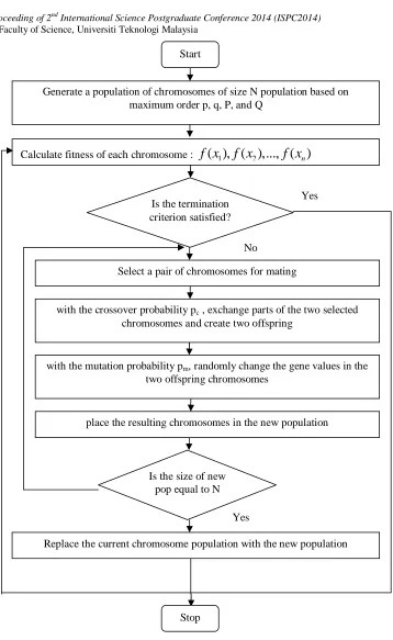
Figure 1 : Research flow of GA procedure Yes

Yes

No

Replace the current chromosome population with the new population Is the size of new

pop equal to N

place the resulting chromosomes in the new population with the mutation probability pm, randomly change the gene values in the

two offspring chromosomes

with the crossover probability pc , exchange parts of the two selected

chromosomes and create two offspring Select a pair of chromosomes for mating

Is the termination criterion satisfied?

Calculate fitness of each chromosome :

f x

( ), ( ),..., ( )

f x

f x

Generate a population of chromosomes of size N population based on maximum order p, q, P, and Q

Start

3.0

SIMULATIONS

AND

RESULTS

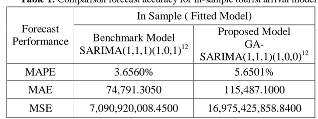
Table 1: Comparison forecast accuracy for in-sample tourist arrival model

Forecast Performance

In Sample ( Fitted Model)

Benchmark Model SARIMA(1,1,1)(1,0,1)12

Proposed Model

GA-SARIMA(1,1,1)(1,0,0)12

MAPE 3.6560% 5.6501%

MAE 74,791.3050 115,487.1000

MSE 7,090,920,008.4500 16,975,425,858.8400

The process of imitating a real phenomenon with a set of mathematical

formulas. Advanced computer programs are used to simulate the tourism

arrival pattern. In theory, any phenomena that can be reduced to mathematical

data and equations can be simulated on a computer. In practice, however,

simulation is extremely difficult because most natural phenomena are subject to

an almost infinite number of influences. For this tourist arrival data, Table 1

shows comparison study between the benchmark model for in-sample tourist

arrival and the proposed GA-BJ model. This study found that forecast accuracy

for benchmark model, SARIMA(1,1,1)(1,0,1)

is 3.656% mean absolute

percentage error while the proposed GA- SARIMA(1,1,1)(1,0,0)

model

produced 5.6501% mean absolute percentage error.

This shows that SARIMA(1,1,1)(1,0,1)

is more accurate compared to

GA-SARIMA(1,1,1)(1,0,0)

in modeling training data. This is due to the local

optima occurs in finding parameter values for GA-BJ model for training data.

Nevertheless, 2% different error is still acceptable to proceed for developing

forecast model.

Figure 2 In-sample benchmark model and proposed model for monthly International tourist arrival to Malaysia.

Table 2 : Comparison forecast accuracy for out-sample tourist arrival model

Forecast

Performance

Out Sample ( Forecast Model)

Benchmark Model

SARIMA(1,1,1)(1,0,1)12

Proposed Model

SARIMA(1,1,1)(1,0,0)12

MAPE 7.1920% 6.8580%

MAE 141,164.58 139,876.82

MSE 30,409,366,540.92 29,311,895,500.32

Table 2 shows forecast accuracy for 12 step ahead monthly international

tourist arrival to Malaysia year 2011. It shows that GA-SARIMA(1,1,1)(1,0,0)

model successfully improved forecasting accuracy for modeling international

tourist arrival to Malaysia with 6.858% mean absolute percentage error

compared to benchmark model, SARIMA(1,1,1)(1,0,1)

is 7.192% mean

absolute percentage error only. Thus, this proposed model can be used as an

alternative way to forecast monthly international tourist arrival.

benchmark model. As can be seen in proposed model, SARIMA(1,1,1)(1,0,0)

has less parameters to be estimated compared to benchmark model,

SARIMA(1,1,1)(1,0,1)

which has four parameters. Thus, it proves that GA can

effectively finds the approximate optimum solution in estimating the orders and

parameters of SARIMA model. This findings is in line with study by

Abo-Hammour [30] which GA technique produced more easy, robust and accurate

forecast model.

Figure 3 Out-sample benchmark and proposed model for monthly international tourist arrival to Malaysia.

General proposed forecast model used

for this study

is

SARIMA(1,1,1)(1,0,0)

with 30 generations, 100 chromosomes and the

general formula is as follow :

1 _{1 11 1 1 1 11 1 12 1 1 1 1 12 1}

t _{t t t t t t t t t}

z

 

Z





Z

 



Z



Z

 

Z





Z

 



Z



a





a



1 _{11 11 12}

1 12

0.3276

0.3323

0.1089

0.3276

0.3323

0.1089

0.3323

t _{t t t t t}

t t t t

z

Z

Z

Z

Z

Z

Z

Z

a

a

 _{  }

 

 

















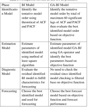
Table 3 : Comparison between BJ and GA-BJ procedures

Phase BJ Model GA-BJ Model Identificatio

n Model

Identify the tentative model order using theoretical of ACF and PACF

Identify the tentative model order by total of maximum 60 significant lags of ACF and PACF then evaluate the best identified model order based on objective function. Estimation Model Estimate parameters of identified model using method of least square algorithm

Estimate parameters of identified model GA-BJ using GA operator and identify the best parameters based on objective function Diagnostic

Model

Evaluate the residual identified BJ model to fulfill characteristics for forecasting

No need to check the residual since identified model checking is filtered base on objective function

Forecasting Choose the best identified model and used for forecasting

Choose the best forecast model based on objective function and forecast performance

As a conclusion, Table 3 concludes the two differences methodological

process of forecasting monthly international tourist arrival to Malaysia.

4.0

SUMMARY AND CONCLUSION

advantage of GAs lies in its flexibility. As long as one decodes the possible

answer in the form of binary strings, one can get the closest result by means of

the evolutionary process of GAs. Reviewing the results of the experimental study

is proved that the searching scheme for best parameters can be found effectively.

Thus, the searching schemes are capable of constructing the evolutionary rule to

achieve satisfactory performance in model identification.

Therefore, a GA method has been proposed successfully for the

identification of BJ model and estimation of the parameters in developing

forecast model for modeling monthly international tourist arrival to Malaysia.

This result is in line with study by Abo Harmour et al [30] who apply time series

modeling using genetic algorithm approach. Hence, the main contributions of

this study are described as follows. First, this research show that the BJ

forecasting model problem can be alternatively solved by the new proposed

combination GA-BJ model based on genetic algorithm and computer

programming language. Second, forecast accuracy of BJ forecast model can be

improved by considering more information on identified model and estimation of

the parameters in BJ procedure using GA method.

Conversely, further research should be considered on other identification

and estimation phase by developing mathematical algorithm in preliminary BJ

analysis. Thus, the raw data can be used automatically in producing GA-BJ

forecasting model. Second, comparison study using other type of forecast

evaluation such as MAPE, MAE, and AIC in evaluating of proposed model

should be considered. Thus, a comprehensive experimental result will be more

accurate in predicting tourist arrival.

In conclusion, this research shows that

combination method is more precise than the single method in order to develop

forecasting model.

A

R

[1]

G. E. . Box and G. Jenkins,

Time Series Analysis, Forecasting and

Control

. Holden-Day, San Francisco CA, 1970.

[2]

H. Song, E. Smeral, G. Li, and J. L. Chen, “Tourism Forecasting

 :,” 2008.

[3]

C. Goh and R. Law, “The Methodological Progress of Tourism Demand

Forecasting: A Review of Related Literature,”

Journal of Travel &

Tourism Marketing

, vol. 28, no. 3, pp. 296–317, Apr. 2011.

[4]

F.-L. Chu, “Forecasting tourism: a combined approach,”

Tourism

Management

, vol. 19, no. 6, pp. 515–520, Dec. 1998.

[5]

J. H. Kim and I. a. Moosa, “Forecasting international tourist flows to

Australia: a comparison between the direct and indirect methods,”

Tourism Management

, vol. 26, no. 1, pp. 69–78, Feb. 2005.

[6]

C. Goh and R. Law, “Modeling and forecasting tourism demand for

arrivals with stochastic nonstationary seasonality and intervention,”

Tourism Management

, vol. 23, no. 5, pp. 499–510, Oct. 2002.

[7]

C. Lim and M. McAleer, “Time series forecasts of international travel

demand for Australia,”

Tourism Management

, vol. 23, no. 4, pp. 389–396,

Aug. 2002.

[8]

V. Cho, “Tourism Forecasting and its Relationship with Leading

Economic Indicators,”

Journal of Hospitality & Tourism Research

, vol.

25, no. 4, pp. 399–420, Nov. 2001.

[9]

H. Hom, “Effect of seasonality treatment on the forecasting performance

of tourism,” vol. 15, no. 4, pp. 693–708, 2009.

[11] J. du Preez and S. F. Witt, “Univariate versus multivariate time series

forecasting: an application to international tourism demand,”

International

Journal of Forecasting

, vol. 19, no. 3, pp. 435–451, Jul. 2003.

[12] F.-L. Chu, “Forecasting tourism demand with ARMA-based methods,”

Tourism Management

, vol. 30, no. 5, pp. 740–751, Oct. 2009.

[13] C.-L. Chang, S. Sriboonchitta, and A. Wiboonpongse, “Modelling and

forecasting tourism from East Asia to Thailand under temporal and spatial

aggregation,”

Mathematics and Computers in Simulation

, vol. 79, no. 5,

pp. 1730–1744, Jan. 2009.

[14] V. Cho, “Tourism Forecasting and its Relationship with Leading

Economic Indicators,”

Journal of Hospitality & Tourism Research

, vol.

25, no. 4, pp. 399–420, Nov. 2001.

[15] E. Smeral, “Does Complexity Matter? Methods for Improving Forecasting

Accuracy in Tourism: The Case of Austria,”

Journal of Travel Research

,

vol. 44, no. 1, pp. 100–110, Aug. 2005.

[16] F. L. Chu, “A fractionally integrated autoregressive moving average

approach to forecasting tourism demand,”

Tourism Management

, vol. 29,

no. 1, pp. 79–88, Feb. 2008.

[17] R. Y. C. Fan, S. T. Ng, and J. M. W. Wong, “Reliability of the Box–

Jenkins model for forecasting construction demand covering times of

economic austerity,”

Construction Management and Economics

, vol. 28,

no. 3, pp. 241–254, Mar. 2010.

[18] C. Chatfield,

Time Series Forecasting

. Chapman & Hall CRC FLorida,

2001.

[19] Z. S. Abo-Hammour, O. M. K. Alsmadi, A. M. Al-Smadi, M. I. Zaqout,

and M. S. Saraireh, “ARMA model order and parameter estimation using

genetic algorithms,”

Mathematical and Computer Modelling of

Dynamical Systems

, vol. 18, no. 2, pp. 201–221, Apr. 2012.

[21] H. Akaike, “Information Theory and an Extension of the Maximum

Likelihood Principle,”

2nd international symposium and information

theory

, 1970.

[22] J. Hannan, E, “The Estimation of the order of an ARMA process,”

Ann.

Stat

, no. 8, pp. 1071–1081, 1980.

[23] J. Hannan, E and G. Quinn, B, “The Determination of the order of an

autoregession,”

J.R.Stat. Soc,. Ser

, pp. 190–95, 1979.

[24] G. Liang, D. M. Wilkes, and J. a. Cadzow, “ARMA model order

estimation based on the eigenvalues of the covariance matrix,”

IEEE

Transactions on Signal Processing

, vol. 41, no. 10, pp. 3003–3009, 1993.

[25] A. S. Association, “On The Relationship Between the S Array and the

Box-Jenkins Method of ARMA Model Identification,”

Journal of the

American Statistical Association

, vol. 375, no. 76, pp. 579–587, 1981.

[26] A. S. Association, “Consistent estimates of autoregressive parameters and

extended sample autocorrelation function for stationary and nonstationary

ARMA models,”

Journal of the American Statistical Association

, vol.

385, no. 79, pp. 84–96, 1984.

[27] G. C. Tiao and R. S. Tsay, “Use of canonical analysis in time series model

identification,”

Biometrika

, vol. 2, no. 72, pp. 299–315, 1985.

[28] E. J. Hannan and J. Rissanen, “Recursive Estimation of Mixed

Autoregressive-Moving Average Order,”

Biometrika

, vol. 69, no. 1, pp.

81–94, Apr. 1982.

[29] C.-S. Ong, J.-J. Huang, and G.-H. Tzeng, “Model identification of

ARIMA family using genetic algorithms,”

Applied Mathematics and

Computation

, vol. 164, no. 3, pp. 885–912, May 2005.

[30] Z. S. Abo-Hammour, O. M. K. Alsmadi, A. M. Al-Smadi, M. I. Zaqout,

and M. S. Saraireh, “ARMA model order and parameter estimation using

genetic algorithms,”

Mathematical and Computer Modelling of