Intelligent active force control of a rigid robot arm using embedded iterative learning algorithm

(1)

Jumal Mekanikal, JilidII.2000

INTELLIGENT ACTIVE FORCE CONTROL OF A RIGID

ROBOT ARM USING EMBEDDED ITERATIVE

LEARNING ALGORITHM

Musa Mailah

Department of Applied Mechanics Faculty of Mechanical Engineering

Universiti Teknologi Malaysia 81310 Skudai, Johor Bahru

MALAYSIA Email: [email protected]

ABSTRACT

The paper presents a novel approach to estimating the inertia matrix of a robot arm adaptively and on-line using an iterative learning algorithm. It is employed in conjunction with an active force control strategy which has been shown to be very effective in accommodating the disturbances. A comprehensive study is performed on a rigid two link manipulator subject to a number of

(2)

Jurnal Mekanikal, Jilid II, 2000

1.0 INTRODUCTION

The control of robot arm has been a subject of active research for the last two decades. A number of control methods has been proposed ranging from a simple classical proportional-plus-derivative (PD) control to the more recent adaptive and intelligent control. The PD control [1] though simple is quite efficient and provide stable performance at very low speed operation and without/little disturbance. The performance, however, degrades considerably at high speed and with the presence of disturbances. Thus, there is a need to overcome this critical limitation as practical application is becoming increasingly difficult, complex and challenging. This gives rise to a class of adaptive control techniques [2,3,4]' which to certain extent successfully improve the stability and robustness of the system by extending the ability to operate in a wider range of parametric or non-parametric uncertainties. However, this often involves complex mathematical manipulations and assumptions. Itis thus common to find that this type of control method is limited to theoretical and simulation study. There is a growing trend in robot control in which intelligent mechanism is incorporated using features such as knowledge-based (expert system) [5], neural network [6,7,8], fuzzy logics [9] and iterative learning algorithm [10,11]. Intelligent robotic system is considered the state-of-the art technology in which the machine is designed to emulate part of human attributes especially in the aspects of learning and decision making. A number of research works in this field demonstrated the advantages of the scheme compared to other methods [11].

In this paper, iterative learning technique is used in conjunction with an active force control (AFC) strategy to control a robot arm.It is shown that the iterative learning control mechanism is able to compute continuously and on-line, the estimated inertia matrix of the robot arm while the AFC component excellently compensates for the disturbances.

(3)

Jumal Mekanikal, Jilid II, 2000

The paper is structured as follows. The first part deals with a description of the problem statement and the fundamentals of both the AFC' and learning control methods. Next, the integration of the iterative learning algorithm and AFC applied to a two link rigid robot arm is demonstrated in the form of a simulation study. This is followed by an analysis and discussion of the results obtained. Experimental work is also carried out to verify the effectiveness of the proposed scheme. Finally, a conclusion is derived and further works which could be carried out are pointed out.

2.0 PROBLEMSTATEMENT

Active force control applied to robot arm is first proposed by Hewit towards the end of seventies [12]. The aim of this type of control method is to ensure that the system is stable and robust even in the presence of known or unknown disturbances. A distinct advantage about this method is the practical realization of the system in which the method bases its concept on using mainly the estimated or measured values of certain parameters to effect its compensating action. This has the benefits of reducing the mathematical complexity of the robot system which is known to be highly coupled and non-linear.

(4)

options - all seemingly aiming towards the incorporation of intelligent

mechanism such as using neural network, fuzzy logics, genetic algorithm,

optimization technique and iterative learning method. Within this framework, and

with a clear direction in mind, a method has been devised which integrates the

intelligent control into the AFC strategy.

The paper describes a novel approach to control a robotic arm using an

iterative learning method coupled to the active force control (AFC) strategy. It is

demonstrated in this paper the effectiveness of the learning algorithm as an

on-line parameter estimator which provide the signal iteratively to the AFC section

for the compensation of the introduced disturbances. As a result, the control

scheme is able to operate within a wide range of parametric and non-parametric

uncertainties. In other words, the proposed system is robust against all forms of

disturbances.

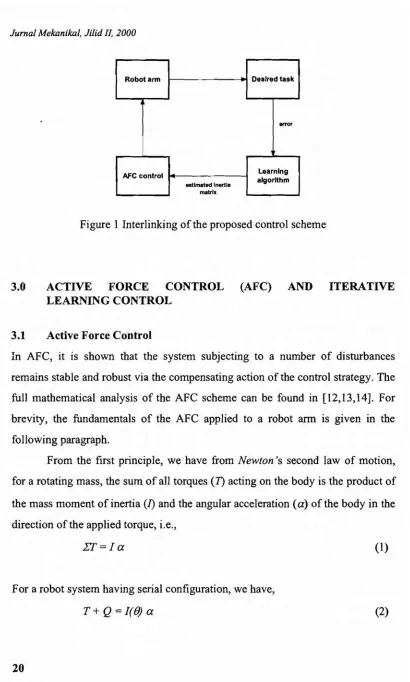
The idea behind the scheme is to obtain a continuous computation of the

estimated inertia matrix of the arm by means of a suitable learning algorithm iri

which the arm is gradually forced to execute a prescribed task accurately even in

the presence of external disturbances. As the arm starts to move the internal

mechanism activates the learning process - identifying new inertia values of the

links at each iteration which is fed into the AFC loop, performing the required

task and eventually reducing the track error. This error is in tum fed back into the

learning algorithm section and the process is repeated iteratively until a suitable

error goal criterion is achieved. Figure I shows a block diagram representing the

interlinking of the proposed control scheme.

To provide better insight to the proposed scheme under study, the

fundamentals of both AFC and the iterative learning methods are briefly

explained in the following sections.

(5)

Jurnal Mekanikal, JilidII, 2000

Robot arm DesIred task

error

AFCcontrol LearnIng estimated Inertl. algorithm

matrix

Figure 1 Interlinking of the proposed control scheme

3.0 ACTIVE FORCE CONTROL (AFC) AND ITERATIVE

LEARNING CONTROL

3.1 Active Force Control

In AFC, it is shown that the system subjecting to a number of disturbances

remains stable and robust via the compensating action of the control strategy. The

full mathematical analysis of the AFC scheme can be found in [12,13,14]. For

brevity, the fundamentals of the AFC applied to a robot arm is given in the

following paragraph.

From the first principle, we have from Newton's second law of motion,

for a rotating mass,the sum of all torques(1) acting on the body is the product of

the mass moment of inertia(I) and the angular acceleration(a) of the body in the

direction of the applied torque, i.e.,

IT=/a

For a robot system having serial configuration, we have,

T+ Q=/(B)

a

(1)

(6)

Jurnal Mekanikal,

nu«

II, 2000

We can obtain a measurement of

Q'

of

Q

as

Q'=J'a '-T' (3)

where the superscript' denotes a measured or computed (or estimated) quantity.

In this context, T' can be easily measured by means of a current sensor and a'

using accelerometer. J' may be obtained by assuming a perfect model or simply

crude approximation.

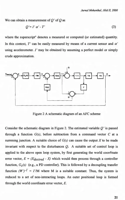
Figure 2 A schematic diagram of an AFC scheme

Consider the schematic diagram in Figure 2. The estimated variable Q' is passed

through a function G(s), before subtraction from a command vector C at a

summing junction. A suitable choice ofG(s) can cause the output X to be made

invariant with respect to the disturbances

Q.

A suitable set of control loop is

applied to the above open loop system, by first generating the world coordinate

error vector, E = (Xdesired - X) which would then process through a controller

function, Gc(s) (e.g.,a PD controller). This is followed by a decoupling transfer

function (W')-l = rIM where M is a suitable constant. Thus, the system is

reduced to a set of non-interacting loops. An outer positional loop is formed

through the world coordinate error vector, E.

(7)

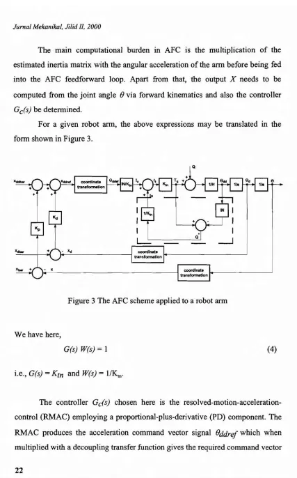
The main computational burden in AFC is the multiplication of the estimated inertia matrix with the angular acceleration of the arm before being fed into the AFC feedforward loop. Apart from that, the output X needs to be computed from the joint angle () via forward kinematics and also the controller Gc(s) be determined.

For a given robot arm, the above expressions may be translated in the form shown in Figure 3.

Figure 3 The AFC scheme applied to a robot arm

We have here,

G(s) W(s)

=

1

i.e., G(s)

=

Ktn and W(s)

=

l/Km·

(4)

(8)

to the main AFC loop. The equation describing the disturbances is given as follows:

(5)

In AFC, we can effectively accommodate the disturbances by obtaining the measurements of the acceleration and the torque using physical accelerometer and torque sensor respectively. More conveniently, we can rewrite Equation (5) (based on the torque-current relationship) in the following form:

(6)

In this way, we can instead measure the controlled current

It

to the motor and obtain exactly the same result. The AFC concept has been successfully implemented to robot arm via simulation and experimental works [16,17,18,19].

The only additional and necessary requirement is the acquisition of an appropriate estimated inertia matrix of the arm to be multiplied with the 'measured' acceleration as in Equation (6). Previous cited works on AFC use traditional techniques which are rather crude, not systematic and mostly based on rough estimation. Thus, it is highly desirable that a method should be devised in such a manner that the inertial parameter can be identified intelligently without having to resort to the conventional approaches described above. A novel method has been proposed here using iterative learning algorithm which is described in the following section. Results obtained through simulation and experimental study demonstrate the effectiveness and simplicity of the proposed method.

3.2 Iterative Learning Control

(9)

robustness [10,20,21,22,23]. In other words, it can be shown that as the number of iterationk(t) increases i.e k-+CXJfor t6[0,

tstop],

the track error e converges to zero (e~O).A suitable algorithm is described in this paper and later implemented to the system under study. A learning algorithm of the following form is chosen:

Yk+]

=

Yk

+

(cj)

+

r

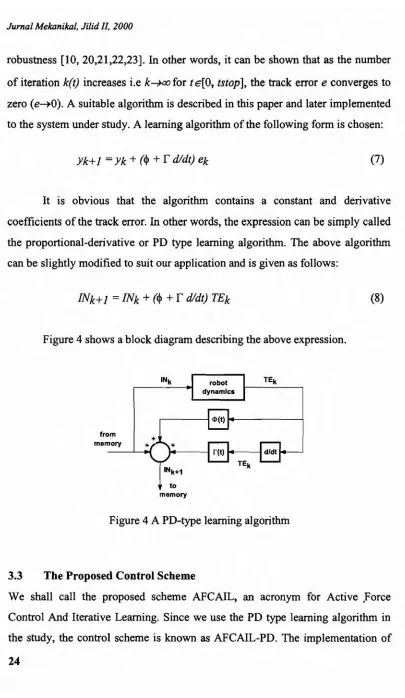
dldt) ek (7)

It is obvious that the algorithm contains a constant and derivative coefficients of the track error. In other words, the expression can be simply called the proportional-derivative or PD type learning algorithm. The above algorithm can be slightly modified to suit our application and is given as follows:

INk+]

=

INk

+

(cj)

+

r

dldt) TEk

Figure 4 shows a block diagram describing the above expression.

from memory

to memory

Figure 4 A PD-type learning algorithm

(8)

3.3 The Proposed Control Scheme

(10)

Jumal Mekanikal, Jilid IL 2000

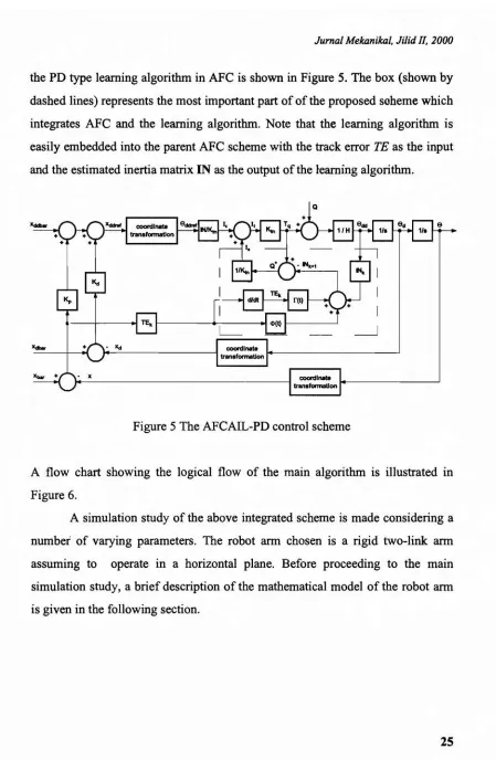
the PD type learning algorithm in AFC is shown in Figure 5. The box (shown by dashed lines) represents the most important part of of the proposed scheme which integrates AFC and the learning algorithm. Note that the learning algorithm is easily embedded into the parent AFC scheme with the track error TE as the input and the estimated inertia matrix IN as the output of the learning algorithm.

.

Figure 5 The AFCAIL-PD control scheme

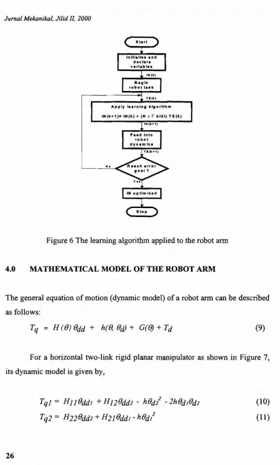
A flow chart showing the logical flow of the main algorithm is illustrated in Figure 6.

A simulation study of the above integrated scheme is made considering a number of varying parameters. The robot arm chosen is a rigid two-link arm assuming to operate in a horizontal plane. Before proceeding to the main simulation study, a brief description of the mathematical model of the robot arm is given in the following section.

(11)

Jumal Mekanikal,Jilid II, 2000

Apply I••rnlng .Igorllhm

IN(k+l)- IN(k) +(eI> +rd/dl) TE(k)

N.

Figure 6 The learning algorithm applied to the robot ann

4.0 MATHEMATICAL MODEL OF THE ROBOT ARM

The general equation of motion (dynamic model) of a robot ann can be described

as follows:

Tq == H (B) Bdd

+

h(fJ, BdJ

+

G(fJ)

+

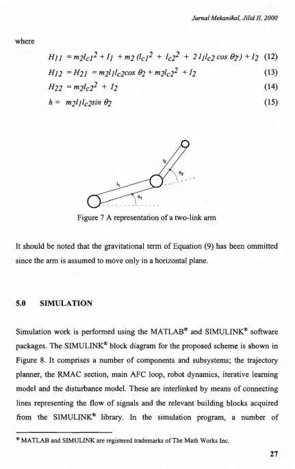
Td (9)

For a horizontal two-link rigid planar manipulator as shown in Figure 7,

its dynamic model is given by,

Tql

=

HnBddl

+

H12 Bdd2 - hBdi - 2hBdlBd2

Tq2

=

H22 Bdd2

+

H21Bddl - hBd/

(10)

(12)

Jumal Mekanikal, JilidII, 2000

where

H11

=

m21el2

+

I]

+

m2 (lel 2

+

_Ic22

+

_{21]lc2 cos B2')}

+

12 (12)

H]2 =H21 =m21]lc2cosB2+m2Ic22 +12 (13)

H22

=

m21c22

+

12 (14)

h

=

m21]lc2sin B2 (15)

Figure 7 A representation of a two-link arm

It should be noted that the gravitational term of Equation (9) has been ommitted since the arm is assumed to move only in a horizontal plane.

5.0 SIMULATION

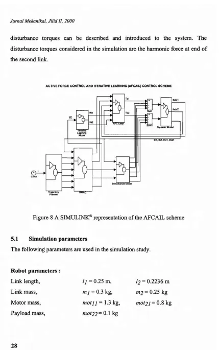
Simulation work is performed using the MATLAB® and SIMULINK@ software packages. The SIMULINK@ block diagram for the proposed scheme is shown in Figure 8. It comprises a number of components and subsystems; the trajectory planner, the RMAC section, main AFC loop, robot dynamics, iterative learning model and the disturbance model. These are interlinked by means of connecting lines representing the flow of signals and the relevant building blocks acquired from the SIMULINK@ library. In the simulation program, a number of

<IllMATLAB and SIMULINK are registered trademarks of The Math Works Inc.

(13)

Jurnal Mekanikal, Ji/idII, 2000

disturbance torques can be described and introduced to the system. The disturbance torques considered in the simulation are the harmonic force at end of the second link.

ACTIVE FORCE CONTROL AND ITERATIVE LEARNING (AFCAIL) CONTROL SCHEME

Figure 8 A SIMULINKIlilrepresentation of the AFCAIL scheme

5.1 Simulation parameters

The following parameters are used in the simulation study.

Robot parameters: Link length,

Link mass, Motor mass, Payload mass,

l I

=

0.25 m,

m]

=

0.3 kg, mot11

=

1.3 kg, mot22

=

0.1 kg

(14)

Jumal Mekanikal, JilidII, 2000

Controller parameters:

Controller gain,

Motor torque constant,

Iterative learning parameters :

Proportional term, Derivative term,

Main simulation parameters:

Integration algorithm Simulation time start, tstart Simulation time stop, tstop Minimum step size

Maximum step size

~=750 Is,

x,

= 0.263 Nm/A

<1>

=

0.005

r

=

0.0075

Gear 0.0 25 s 0.01 0.1

K

=

500

Is

2 d

The gain constants,

K,.

and K, of the control scheme are assumed to be satisfactorily tuned heuristically prior to the simulation work. The motor torque constant Km=0.263 Nm/A is obtained from the actual data sheet for the DC torque motor. Simulation is performed first without considering any external disturbances acting on the system. Later, the applied disturbance is assumed.

5.2 The Initial Conditions

In this study, we consider the initial state of the estimated inertia matrix of the arm to start from 0 kgrrr or specifically IN] = 0.0 kgrrr andIN2 = 0.0 kgrrr'. In other words, no prior knowledge of the inertial parameter is assumed - which is a very important contribution of the research work.

(15)

Jurnal Mekanikal, Jilid II. 2000

5.3 The Sample Time

The sample time instant for the learning algorithms is set to O.Ols. This implies that the next step value ofIN is updated every O.Ols, i.e., if the initial value of INk(initial k=0) is 0 s then the next value _INk+1 is sampled at O.Ols and so forth.

For the purpose of the analysis of the results obtained, rather than using iteration number, it is preferred that the description of the convergence of the algorithms is based on the number of cycles of the circular trajectory generated which is calculated from the time it takes for the trajectory to complete a perfect circle (for the simulation this time is calculated to be t_e =3.14 s). Thus, 2 cycles would be 2*t_e,5 cycles is 5*t_eetc.

5.4 The Stopping Criteria

A stopping criterion should be specified especially if convergence of the desired parameter (or learning) has taken place. In this paper, we consider a suitable elapsed time of 25s or approximately 8 cycles (8td of a complete circular trajectory as the stopping mechanism so that the behaviour of the system can be observed and critically analyzed especially on-line.

5.5 The Prescribed Trajectory

A prescribed circular trajectory as shown in Figure 9 is considered in the simulation study. The trajectory is generated using the following time (t) dependent functions:

Xbarl = 0.25

+

0.1 sin (Veut tiD. 1) xbar2 = 0.1

+

0.1 cos(Veut tiD. 1)

(16)

Jurnal Mekanikal, JilidII.2000

Desired trajectory of the ann

0.5 .---,r---'--=----.---,

0.4 . __ __.;. __ ; .

0.6 0.4

0.2

;~I::([J'

· .

x,(m)

Figure 9 The desired trajectory of the arm

5.6 The Applied Disturbances

An explicit account of the effect of the disturbances applied to the robot arm is given. This is performed to investigate the robustness of the proposed scheme. The simulation is first carried out without considering any external disturbances acting on the system. Later, we introduce a harmonic force which is applied at the end of second link. We have the harmonic force,

Fh

=

h sint where the magnitude of force is h

=

30 N.

(18)

6.0 RESULTS AND DISCUSSION

Figure 10 and 11 show the detailed results obtained through the simulation work. The graphical results are related to the trajectory obtained, the track error produced, the estimated inertia matrix computed and the resulting torque actuated.

(17)

Jumal Mekanikal, Jilid II. 2000

Trajectoryafter1cycle Trajectoryafter7cycles 10.--~~_~~_ ___,

0.3:> 0.25 :§:uzo >f' 0.15 0.10 0.3:> 0.25 :§:O.~ >f' 0.15 0.10

0.15 O.~ 0.25 0.3:> 0.35 0.4 X,(m)

(a)

0.15 O.~ 0.25 0.3:> 0.35 0.4 X,(m)

(b)

0.010 . - - -,

4 0 . - - - ,

O.lXXl+--r--,-r'--T"""T-r"""'T"""T-I

-Tq1

- - - Tq2

3:>

l~ ~ 10

~ 0-+- _

i

-10

8

.~ -3:> IN1=1N2 'f0.OO8 ~.006 ;;;:; alO.OO4

~O.~

5 10 m ~ 25 0 5 10 m ~ 25

1(5) t(s)

W 00

Figure 10 Results for the AFCAIL-PD scheme, no disturbance, Fa

0.3:> 0.25 :§:O.~ >f' 0.15 0.10

TrajectOlVafter1cycle

o

I

0.15 uzo 0.25 0.3:> 0.35 0.4 X,(m) (a) 03) 0.25 :§:ozo >f' 0.15 0.10

Trajectoryafter7cycles

0.15 ozo 0.25 0.3:> 0.35 0.4 X,(m)

(b)

:J)'r-~~_~~_-,

~-Tq1

Tq2

10 15 zo 25

l(s)

o

40 ...- - - ...,

3:>

!~ ~ 10

~ 0 '

1'10

8'~ -3:>

IN1=1N2

o 5 10 15 ~ 25

1(5)

0.00-4-...-r-r-r-T-r--r-,...,.-!

O.lE . . .- -,

W 00

(18)

Jurnal Mekanikal, Ji/id II, 2000

Itis obvious that the learning process is accomplished gradually with the initial generated trajectory appearing distorted and disoriented. Figure lO(a) and 11(a) show the actual trajectories of the arm after the robot performs 1 complete cycle of trajectory tracking. As the iteration proceeds, the eventual trajectory almost replicates the desired one, signifying that learning process has indeed ocurred. This is especially observed after the learning has reached 7 cycles as depicted in Figure lO(b) and ll(b). The track error curves confirm this fact - the initial stage is characterized by very large error but as learning takes place, the track error is observed to continually and gradually decrease and this applies for all conditions considering with or without external disturbances as shown in Figure IO(c) and 11(c). In addition to that, it is also noticed that the pattern of the trajectory track error corresponds to the types of external disturbances applied to the system.

The proposed control scheme is shown to have fast learning characteristic - the trajectory track error for all the cases dips to below the 2.5 mm margin at the end of the simulation period. The gradual mapping of the trajectory to the desired one is found to be smooth and the final track error is acceptably small.

Generally, the computed IN for all the cases, is seen to rise steadily and upwardly from the given initial conditions as shown in Figure lO(d) and 11 (d). The initial state of the inertia matrix is characterized by a sharp jump to a value which more or less stabilizes and later gradually and steadily increases in a non-linear fashion as iteration continues and the learning rule computes new value of IN for the next sample instant.Itis essential to ensure thatIN should be positive definite which would otherwise causes the system to become unstable. The choice of suitable learning parameters (~ and f) for the learning rules is also important as this affects the slope of the IN curve. For instance, inappropriate value of the parameters would cause the gradient of IN curve to increase dramatically and thus lead to instability. A slight and gradual increase in the slope would be sufficient to yield a very good response. A number of trials is

(19)

performed to determine the value of these constants and the results suggested that the values assumed are acceptable.

It is also obvious that the inertia matrix varies with the type of applied disturbances. The IN curve shows small fluctuating pattern corresponding to the harmonic input as hown in Figure II(d).

6.1 Initial Value of the Estimated Inertia Matrix

A significant and indeed a desirable feature of the employed learning scheme is realized when the initial estimated inertia matrix is assumed to be of the same value. This implies that only a single value of the estimated inertia matrix is needed to perform the required task. Thus, by putting the initial value IN]=IN2 =0.0 kgm', we have both the computed values to be exactly the same and yet producing stable performances with the trajectory track error reduced to acceptable tolerance. This has the added advantage in terms of less computation is required to determine IN especially if the degrees of freedom of the arm is greater than two. In this context, we can assume all the diagonal terms of the inertia matrix to be of the same value. As far as the two-link arm is concerned, the simulation results indicate that the assumption is valid.

Thus, as an example, for a three degree of freedom robot arm, we may have,

(19)

where IN]=IN2=IN3 assuming that the learning algorithm has optimized' the IN.

(20)

6.2 The Computed Inertia Matrix

The computed estimated inertia matrix varies in a range of values as summarized

in Table I.

Table I Range of computed estimated inertia matrix

Types of Range of computed IN

disturbances IN]

=

IN2 (kgm")

No disturbance,

F

_o 0.0 - 0.007

Harmonic force,

Fh

0.0 - 0.042

From the table, it can be seen that the range of IN varies positively from 0

kgm" to a maximum value of 0.042kgrrr'. The harmonic force produces higher IN

due to the fact that the force is continuously acting on the system.In other words,

IN is influenced considerably by the nature of the forces applied. The robot arm

responds to these disturbances by adaptively updates the IN via the control

strategy. Since the error is considered 'minimum' at the end of the simulation

period, this corresponds to the optimum value of the computed IN. On the whole,

even though there is a variation in the computed IN for different cases, the results

have clearly indicated that the trajectory track error converges to acceptable value

signifying that the system is very stable and robust. It also suggests that the

intelligent mechanism has successfully adapted the inertial parameter to the

changes in the environment. The other reason is attributed to the fact that the

AFC scheme is very tolerant to variation in the estimated inertia matrix - which

somehow explains the successful implementation of AFC by using only crude

approximation.

An interesting feature can be derived from the study - we can identify a

'safety zone' for a range of suitable IN. We know that as learning progresses, IN

approaches the tolerable range in which the system behaves robustly even in the

(21)

. Jurnal Mekanikal,JilidIl, 2000

presence of large external disturbances. We can determine this range by

observing the characteristics of the trajectory track error from which an error

margin can be specified and thus, a range of IN values can be easily determined.

As an example, by assuming a starting error margin, we can obtain the

corresponding time t it occurs and then relates it to the IN curve.Figure 12(a) and

(b) shows how this is accomplished.By setting the track error TE to 6.0 mm, we

project a line (dashed lines) to the horizontal axis and obtain t to be about 3.8 s.

Referring to the IN curve at time /=3.8 s, we have IN value equals 0.018 kgrrr'.

This can be regarded as the starting IN at which the system behaves stably and

robustly. The other extreme end of the range can be obtained by extending the

simulation time to such an extent that the.error margin increases dramatically or

when the system starts to behave awkwardly or erratically.

Computed IN,and IN,

, . . .

0.04 : ; ~ ; ..

0.05.----,----'-r--.:...,----=----r---,

Trajectory track error

0.011!+-_--,-_...:-,,----;._-,--_ _ ,_ _- . ,

. .

0.008 : : ; ; __

25

IN O.OJ ~ i.... ..';" ~ .

Ikgm') ;_. _. : :

.

_.

0.02 : ; ~ ; .

I : . . .

0.01 l..; i ; ; . I : : : :

I : . : :

I : : :.

5 10 15 20

t(5)

(a) (b)

Figure 12 Determining the 'safety zone'

6.3 The Actuated Torques

Itcan be seen that the controlling torque varies non-linearly and is influenced by

the disturbances applied (see Figure 10(e) and 11(c)).In this study, the saturation

(22)

robustness against large forces. The saturation value of the torque can be easily calculated from the following equation:

(20)

From the actual data sheet, K, is found to be 0263 Nm/A and the maximum permissible motor current is 12.3A. Thus the maximum torque is ±3.3 Nm. In practice, this value must be kept within the maximum allowable limit to avoid damage to the motor. From the results, it can be deduced that, apart from the case where there is no disturbances acting on the robot ann, others with various applied disturbances produce torques which are by far greater than the saturated value. This implies that the AFC scheme is excellent in 'cancelling' the disturbances even though the forces present are much larger than the system can physically tolerate. Itis also obvious that the controlling torque at the first joint is greater than that at the second joint, i.e,

T

_{q]>Tq2. This may be contributed to}

the coupling effect of the ann and the accumulated load with respect to the first joint.

7.0 EXPERIMENTAL RESULTS

An experiment was carried out using a single link robot arm as shown in Figure 13. We use a non-linear spring of unknown stiffness attached to the tip of the ann as the force controlled element.

(23)

Figure 13 A view of the experimental robot arm with a spring attached to the tip of the link

The following parameters were used in the experiment :

~= 115, K;=20, Kd=1

x,

=

0.3387Nm/A

Learning parameter: <I>

=

0.05, I'= 0.0001

A sinusoidal input with peak amplitude of 0.1745 rad.

(24)

(2)

---- NC/IL

Q3) - r e R D

0.15 0.10

!

().(!j

CP

0.00

f

-'1l!i -'110 -'115

~

0.0 as 1.0 1.5 2.0

t (5)

(a) Trajectory

G O I r - - - ,

1(1}

(b) Track error

lllIDl,--- -,

(c) Estimated inertia

" , - - - ,

I(oj

(d) Torque

Figure 14 Experimental results

This is verified by observing the characteristic of the track error curve in

(b) which shows the corresponding gradual decrease in the error. The learning

algorithm is evidently forcing the track error to converge to values approaching

the zero datum as time increases. It is also noted that the curve of the estimated

inertia of the arm (c) follows the same pattern to that the track error curve, which

(25)

Jumal Mekanikal, Ji/id II, 2000

is understandable since the estimated inertia matrix is a function of the track error according to the learning rule in Equation (8). The varying inertias of the arm are obviously having positive values as expected from the theoretical point of view. The maximum inertia occurs at the beginning of the cycle which is approximately 0.01 kgm'. The value drops to around 0.0025 kgm' at t

=

2.1 s. We can calculate the average inertia value to be 0.00032 kgm', The torque curve can seen to vary in sinusoidal fashion peaking at approximately ±0.6 Nm. Again we can see that the initial stage is governed by the high oscillatory feature of the torque prior to the learning process

We can deduct" that the iterative learning control algorithm has been effectively and successfully incorporated into the AFC scheme without any difficulty. The learning process is found to be very fast; about 1 s for the sinusoidal responses. Itis thought that one of the contributing factors that makes it easy to be implemented is due to the fact that the actual inertia of the arm is comparatively small (about 0.002 kgnr'). Since IN is assumed to start at 0 kgrrr' and the characteristic of the proposed learning algorithm is such that it only computes positive values (IN>O) at every successive trials, the outcome is expectedly to be very favourable. Thus, the experimental results obtained verify the above condition.

8.0 CONCLUSION

(26)

range of estimated inertia values supplied iteratively by the learning algorithm. Thus the 'twinning' of both the learning and AFC schemes proves to be compatible and very feasible. The learning of the system is reasonably fast - it takes about 25 s to produce an error margin of below 2.5 mm. A significant feature of the proposed scheme is that only a single value of the estimated inertia matrix IN can be used for the same initial condition. This implies less computational burden since the scheme is considered to have optimized the value of computed IN for the robot ann. The experimental results prove the viability and the effectiveness of the proposed control scheme and also illustrate the ease of embedding the learning rule in the parent AFC section. The performance of the scheme should be further investigated, considering a number of varying parameters such as the changes in the payload mass, learning parameters, initial values of IN, types of disturbances and other prescribed trajectories

NOTATION:

ek current positional error input given by ek

=

Xd - Xk G vector of the gravitational torques

H NxNdimensional manipulator and actuator inertia matrix H vector of the Coriolis and centrifugal torques

I mass moment of inertia of the link

f(O) mass moment of inertia of the robot ann and () is the robot joint angle

IN estimated inertia matrix

INk current value of the estimated inertia matrix INk+l next step value of estimated inertia matrix

It

armature current for the torque motor K, motor torque constant

( vector of link lengths

(27)

lc vector of link lengths from the joint to the centre of gravity of link m vector of link masses

Q

disturbance torques T applied torque

Td vector of the external disturbance torques

T

'd"

estimate of all the disturbance torques

TEk current root of sum-squared positional track error, TEk

=

V(

x_barx

_kJ

2

T_q applied control torque Tq vector of actuator torques Yk current (k) output value Yk+ 1 next step value of the output

a angular acceleration of the robot arm

4>,

T suitable constants or learning parameters

0d vector ofjoint velocity Odd vector ofjoint acceleration

REFERENCES

1. Groover, M.P., Weiss, M., Nagel, R.N., and Odrey, N.G., Industrial Robotics: Technology, Programming and Applications, McGraw-Hill Book Co., 1986.

2.

Slotine,

lE.

and Li, W., Adaptive Manipulator Control: A Case Study, IEEE Transactions on Automatic Control, Vol. 38, No. 11, November

(28)

3. Sinha, A.S.C., Kayalar, S. and Yourtseven, H.O., Nonlinear Adaptive

Control of Robot Manipulators, IEEE Transaction on Robotics and

Automation,Vol. 2, 1990, pp 2084-2087.

4. Tomizuka, M. and Yao, B., Adaptive Control of Robot Manipulators in

Constrained Motion - Controller Design, Transactions of the ASME,

Journal of Dynamic Systems, Measurement and Control, Vol. 117,

September 1995, pp 321-328.

5. Shibata, T., Fukuda,

I.,

Shiotani, S., Mitsuoka T., and Tokita, M.,

Hiearchical Hybrid Neuromorphic Control System, JSME International

Journal, Series C, Vol. 36, No.1, 1993, pp 100-109.

6. Kawato, M., Uno, Y., Isobe, R., .and Suzuki, R, Hiearchical Neural

Network Model For Voluntary Movement With Aplication to Robotics,

IEEE Control Systems Magazine (8), 1988, pp 8-15.

7. Goldberg,K. and Pearlmutter, B., Using A Neural Network to Learn the

Dynamics of the CMU Direct-Drive

Arm

II, Technical Report CMU

-CS-88-160,Carnegie Mellon University, Pittsburgh, August, 1988.

8. lung, S. and Hsia,

I.e.,

A New Neural Network Control Technique For

Robot Manipulators, Robotica (1995), Vol. 13, pp. 477-484, 1995.

9. Ohnishi, K., Shibata, M. and Murakami, T.,A Unified Approach to Position

and Force Control by Fuzzy Logic, IEEE Transactions on Industrial

Electronics, Vol. 43, No.1, February 1996, pp 81-7.

10. Arimoto, S., Kawamura, S. and Miyazaki, F., Bettering Operation of

Robots by Learning,Robotic Systems, 1984, pp 123-140.

11. Bondi, P., Casalino, G., and Gambardella, On the Iterative Learning

Control Theory for Robotic Manipulators, IEEE Journal of Robotics and

Automation,Vol. 4, No.1, February 1988, pp 14-22.

12. Astrom, K.J. and McAvoy, T.J., Intelligent Control : An Overview and

Evaluation, David A. White, Donald A. Sofge, Eds., Handbook of

(29)

Jumal Mekanikal, Ji/id II, 2000

Intelligent Control : Neural, Fuzzy and Adaptive Approaches, Van

Nostrand Reinhold, New York, 1992, pp. 3-34.

13. Hewit, J.R., and Burdess, J.S., Fast Dynamic Decoupled Control for

Robotics Using Active Force Control, Mechanism and Machine Theory,

Vol. 16, No.5, 1981, pp. 535-542.

14. Hewit, J.R., and Burdess, J.S., An Active Method for the Control of

Mechanical Systems in The Presence of Unmeasurable Forcing,

Transactions on Mechanism and Machine Theory, Vol. 21, No.3, 1986, pp

393-400.

15. Hewit, J.R., Advances in Teleoperations, Lecture Notes on Control

Aspects, CISM, May 1988.

16. Hewit, J.R., and Bouazza-Marouf,

K.,

Practical "Control Enhancement via

Mechatronics Design, IEEE Transactions on Industrial Electronics, Vol.

43, No.1, February 1996, pp 16-22.

17. Hewit, J.R., Disturbance Cancellation Control, Proc. of Int'l. Conference

on Mechatronics, Turkey, 1996, pp.l35-143.

18. Filippi, E., Experimental Robot Arm, Technical Report, Loughborough

University of Technology, Loughborough, 1993.

19. Jones, C., Robot Control, B.Eng. Thesis, University of Dundee, Dundee,

1995.

20. Arimoto, S.., Kawamura, S., and Miyazaki, F., Bettering Operation of

Robots by Learning, Robotic Systems, 1984, pp 123-140.

21. Arimoto, S., Kawamura, S., and Miyazaki, F., Hybrid PositionIForce

Control of Robot Manipulators Based On Learning Method, Proc. of Int '1.

Can/ on Advanced Robotics, 1985, pp 235-242.

22. Arimoto, S., Kawamura, S., and Miyazaki, F., Applications of Learning

Method For Dynamic Control of Robot Manipulators, Proc. of 24th Conf.

(30)

23. Arimoto, S., Kawamura, S. and Miyazaki, F., Convergence, Stability and

Robustness of Learning Control Schemes for Robot Manipulators, Recent

Trends in Robotics: Modelling, Control and Education, ed. by Jamshidi,

M.,Luh, L.y'S.,and Shahinpoor, M., 1986, pp 307-316.