ABSTRACT
GUO, JIANHUA. Adaptive Estimation and Prediction of Univariate Vehicular Traffic Condition Series. (Under the direction of Dr. Billy M. Williams)
Aimed at providing the anticipatory ability for the proactive traffic control systems, a
new adaptive online short-term univariate traffic condition forecasting method is presented in
this dissertation by assimilating knowledge from previous research. Using 15-minute traffic
flow series as a representative, this methodology is based on the hypothesis that the first two
conditional moments of univariate traffic flow series can be modeled as a
SARIMA+GARCH structure, based on which an online forecasting system can be developed
using seasonal exponential smoothing and Kalman filter. Supplementary components,
including missing value imputation and outlier detection, can be incorporated into the system
to meet the requirements of real traffic data collection situations.
The development of the system follows two steps. In step (1), the SARIMA model is
separated into a seasonal component handling traffic flow level due to historical traffic
information, and a short-term component handling local variation after the traffic level due to
historical information is subtracted. The seasonal component is processed using seasonal
exponential smoothing by recognizing the theoretical equivalence between ARIMA model
and exponential smoothing; the local variation is processed using Kalman filter by
constructing a state space model. Afterwards, GARCH model is processed using Kalman
filter based on the recognition that GARCH has an equivalent representation as ARMA in the
sense of squared series. In step (2), missing values are replaced with one-step-ahead
Outliers, indicating extraordinary patterns, are detected based on intervention analysis and
likelihood ratio test. Outliers are proved to be assimilated into the system through an
investigation showing outliers do have significant influences on the forecasting system.
Additionally, the square root transformation is applied in the system.
Using real traffic operation data from four regions, the research hypothesis is validated
and the proposed methodology is implemented and proved to bear desirable attributes,
including competencies, adaptability, computational efficiency, robustness, and
ADAPTIVE ESTIMATION AND PREDICTION OF UNIVARIATE VEHICULAR TRAFFIC CONDITION SERIES
by
JIANHUA GUO
A dissertation submitted to the Graduate Faculty of North Carolina State University
in partial fulfillment of the requirements for the Degree of
Doctor of Philosophy
CIVIL ENGINEERING
Raleigh
2005
APPROVED BY:
(Dr. Nagui M. Rouphail)
(Dr. Joseph E. Hummer)
(Dr. Peter Bloomfield)
Chair of Advisory Committee
BIOGRAPHY
Jianhua Guo was born in eastern China on May 5, 1976. He started his career in civil
engineering from 1993 when he was admitted into Southeast University in China. He
received a B.S. and a M.S. in 1997 and 1999, respectively. After receiving a Ph.D. at North
Carolina State University, he would like to pursue a research career in transportation
engineering. His research interests mainly focused on applications under the broad umbrella
ACKNOWLEDGEMENTS
I would like to express my sincerest gratitude for having the opportunity to complete this
dissertation. In the trials and tribulations of this process, it would never be possible without
the support, guidance, encouragement, and confidence in me from my advisor Dr. Billy M.
Williams. I aspire someday to reach a modicum of his personal and professional stature.
I want to thank Dr. Peter Bloomfield, Dr. Nagui M. Rouphail, and Dr. Joseph E. Hummer
for severing on my advisory committee. I am indebted to Dr. Bloomfield for the suggestions
and discussions on the statistical analyses in this dissertation. I admire his keen insight and
broad knowledge in statistics. I am grateful to Dr. Rouphail for his help in my course work
and the constructive suggestions on this dissertation that improve its quality greatly. My
special thank goes to Dr. Hummer who stands on my committee for the entire community of
traffic engineers. His challenges and comments benefit this dissertation and will benefit my
future research career as well.
My thanks also go to Shashank Shekhar for discussing and sharing ideas on traffic
forecasting; to Angshuman Guin, through whose work I benefit a lot; to Ting Yi and Jisun
Lee for working together.
I thank the generous sharing of the archived traffic operations data to the third party
researchers as the author by the Minnesota Department of Transportation through the
University of Minnesota at Duluth, the Washington State Department of Transportation
through the Intelligent Transportation Systems Research Program at the University of
through the Center of Advanced Transportation Technology Laboratory at the University of
Maryland. I also thank the United Kingdoms Highways Agency for providing the traffic data
used in this research. The author takes all the responsibility on the analyses and views
presented in this dissertation.
Finally, I would like to take this opportunity to express my thanks to my family for
always being with me. Their unconditional and endless love and insurmountable faith in me
TABLE OF CONTENTS
LIST OF TABLES X
LIST OF FIGURES XIV
LIST OF ABBREVIATIONS XVII
CHAPTER 1 BACKGROUND, MOTIVATION, AND ORGANIZATION 1
1.1 BACKGROUND 1
1.2 MOTIVATION 4
1.3 THESIS ORGANIZATION 5
CHAPTER 2 PROBLEM STATEMENT 7
2.1 GENERAL SHORT-TERM TRAFFIC FORECASTING PROBLEM DEFINITION 7
2.2 IDEAL SHORT-TERM TRAFFIC FORECASTING METHODS 15
2.3 SPECIFICATIONS OF PROPOSED ALGORITHM IN THIS STUDY 19
2.4 SUMMARY 23
CHAPTER 3 LITERATURE REVIEW 24
3.1 CLASSIFICATION OF FORECASTING METHODS 24
3.1.1 Heuristic Methods 24
3.1.2 Linear Statistical Methods 25
3.1.3 Nonlinear Methods 26
3.1.4 Hybrid Methods 27
3.1.5 Traffic Flow Theory Based Methods 28
3.1.6 Adaptive Forecasting Methods 29
3.1.7 Other Methods 30
3.2 METHODOLOGICAL HIGHLIGHTS OF FORECASTING METHODS 30
3.2.1 Random Walk 30
3.2.2 Historical Average 31
3.2.3 Informed Historical Average 31
3.2.5 Univariate Box-Jenkins Method 32
3.2.6 Exponential Smoothing 39
3.2.7 Spectral Representation Analysis 40
3.2.8 VARIMA And STARIMA 42
3.2.9 Transfer Function Model - ARIMAX 42
3.2.10 Neural Network Approach 44
3.2.11 K-Nearest Neighbor 46
3.2.12 Local Linear Regression 47
3.2.13 Kernel Smoothing 48
3.2.14 ATHENA 48
3.2.15 KARIMA 49
3.2.16 Prediction Combination 49
3.2.17 Traffic Flow Theory Method 50
3.2.18 Recursive Least Square 51
3.2.19 Least Mean Square Method 54
3.2.20 Kalman Filter 55
3.2.21 General Linear Model 57
3.2.22 Gaussian Maximum Likelihood Formulation 57
3.3 ROBUST FORECASTING REVIEW 59
3.3.1 Missing Value Imputation 59
3.3.2 Outlier Detection 60
3.4 SUMMARY 62
CHAPTER 4 METHODOLOGY 64
4.1 RESEARCH HYPOTHESIS 65
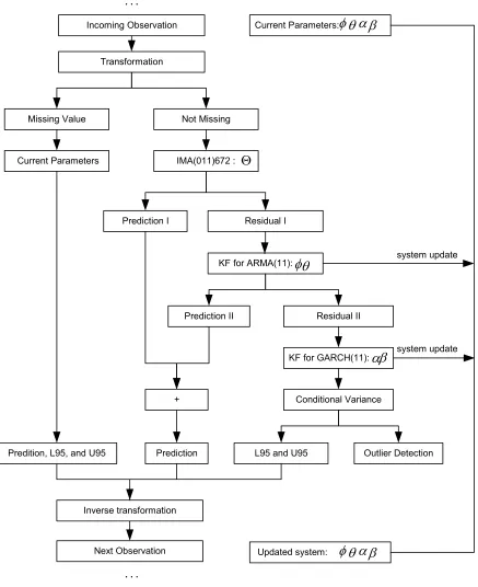
4.2 PROPOSED METHODOLOGY STRUCTURE 68
4.3 TRAFFIC DYNAMICS INVESTIGATION 70
4.3.1 Transformation Selection 71
4.3.2 Conditional Mean Model: SARIMA 73
4.3.3 Conditional Variance Model: GARCH 76
4.4 METHODOLOGY DEVELOPMENT 78
4.4.1 SARIMA Conversion 79
4.4.2 GARCH Conversion 84
4.4.3 Supplementary Components Development 85
4.5 PERFORMANCE MEASURES 86
4.5.2 Measures of Prediction Confidence Interval 90
4.6 SUMMARY 93
CHAPTER 5 DATA DESCRIPTION AND PREPROCESSING 94
5.1 DATA DESCRIPTION 94
5.1.1 UK Motorway Data 94
5.1.2 Washington State Data 97
5.1.3 Maryland Data 99
5.4.4 Minnesota Data 100
5.2 TRAFFIC DATA PRE-PROCESSING 102
5.2.1 Microscopic Validation 102
5.2.2 Traffic Flow Aggregation 103
5.2.3 Macroscopic Validation 105
5.3 TRAFFIC CONDITION ILLUSTRATION 105
5.4 SUMMARY 110
CHAPTER 6 EMPIRICAL STUDY 111
6.1 OBJECTIVES OF EMPIRICAL STUDY 111
6.2 EXPERIMENTAL DESIGN 113
6.2.1 Traffic Dynamics Investigation 114
6.2.2 Forecasting System Development 115
6.3 TRAFFIC DYNAMICS INVESTIGATION 116
6.3.1 Changing Variance Test And Modeling 117
6.3.2 Transformation Analysis 125
6.3.3 Results Illustration 135
6.4 BASIC SYSTEM DEVELOPMENT 143
6.4.1 Implementation 143
6.4.2 Transformation Analysis 144
6.4.3 Sensitivity Analysis 154
6.5 BASIC SYSTEM EVALUATION 155
6.5.2 Prediction Confidence Interval Comparison 159
6.6 FULL SYSTEM DEVELOPMENT AND INVESTIGATION 162
6.6.1 Full System Implementation 163
6.6.2 Adaptability 164
6.6.3 Robustness 174
6.6.4 Transferability 176
6.6.5 Results Illustration 179
6.7 SUMMARY 184
CHAPTER 7 CONCLUSIONS 186
7.1 SUMMARY 186
7.2 MAJOR RESEARCH FINDINGS 187
7.3 RECOMMENDATIONS FOR FUTURE RESEARCH 189
REFERENCES 192
APPENDIX A TRAFFIC DYNAMICS INVESTIGATION 199
APPENDIX B BATCH MODE SYSTEM PERFORMANCE 204
APPENDIX C BASIC SYSTEM PERFORMANCE 227
APPENDIX D FULL SYSTEM PERFORMANCE 250
APPENDIX E COMPARATIVE METHODS PERFORMANCE WITHOUT MISSING
VALUES AND OUTLIERS 253
APPENDIX F COMPARATIVE METHODS PERFORMANCE WITH MISSING VALUES
AND OUTLIERS 259
APPENDIX G SENSITIVITY PLOTS FOR BASIC SYSTEM PARAMETERS 261
APPENDIX H TRANSFORMATION INVESTIGATION FOR FULL SYSTEM 268
APPENDIX I SENSITIVITY PLOTS FOR AKF MEMORY 270
LIST OF TABLES
Table 3.1: Overview of Short-Term Traffic Forecasting Methods 63
Table 4.1: Transformation Descriptions 72
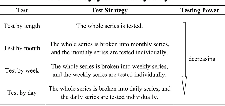
Table 4.2: Changing Variance Testing Strategies 77
Table 4.3: Prediction Confidence Interval Summary Statistics 91
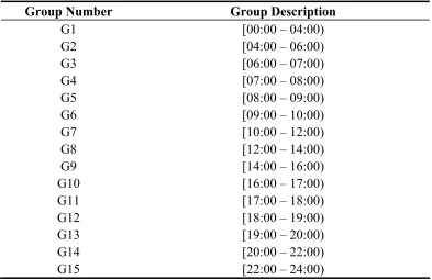
Table 4.4: Groups for Prediction Confidence Interval Evaluation by Traffic Level 92
Table 4.5: Groups for Prediction Confidence Interval Evaluation by Time of Day 93
Table 5.1: Station Description for 1996 UK Data 96
Table 5.2: Station Description for 2002 UK Data 96
Table 5.3: Station Description for WS Data 99
Table 5.4: Station Description for 2004 MD Data 99
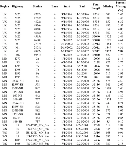
Table 5.5: Station Description for 2000 and 2004 MN Data 102
Table 5.6: Threshold Test for Microscopic Data Validation 103
Table 5.7: Traffic Condition Based on Occupancy Group 106
Table 5.8: Overview of Selected Traffic Flow Data 107
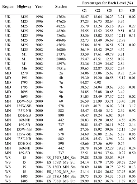
Table 5.9: Traffic Condition Illustration Using Traffic Flow Levels 108
Table 5.10: Traffic Condition Illustration Using Occupancy Data 109
Table 6.1: Transformations for Stations 118
Table 6.2: Results of Heteroscedasticity Testing by Month 121
Table 6.3: Results of Heteroscedasticity Testing by Week 122
Table 6.4: Results of Heteroscedasticity Testing by Day 123
Table 6.5: Repeated t-test for Batch Mode Forecasting Performance 126
Table 6. 7: Results of Prediction CI Width to Flow Ratio by Traffic Level Comparison 129
Table 6.8: Results of Prediction CI Kickoff Percentage by Time of Day Comparison 131
Table 6.9: Results of Prediction CI Width to Flow Ratio by Time of Day Comparison 132
Table 6.10: Transformations for Best Forecasting Performance Measures 134
Table 6.11: Data Selected for Results Illustration 135
Table 6.12: Parameters and Initial Conditions for Basic System 143
Table 6.13: Repeated t-test for Basic System Forecasting Performance 145
Table 6.14: Comparison Results of Basic System Prediction Confidence Interval Kickoff
Percentage by Traffic Level 148
Table 6.15: Comparison for Basic System Prediction Confidence Interval Width to Flow Ratio
by Traffic Level 148
Table 6.16: Comparison Results of Basic System Prediction Confidence Interval Kickoff
Percentage by Time of Day 150
Table 6.17: Comparison Results of Basic System Prediction Confidence Interval Width to
Flow Ratio by Time of Day 151
Table 6.18: Transformations for Best Forecasting Performance Measures of Basic System 153
Table 6.19: Forecasting Performance Comparison Results 158
Table 6.20: Comparison Results of Prediction CI Kickoff Percentage by Traffic Level 160
Table 6.21: Comparison Results of Prediction CI Width to Flow Ratio by Traffic Level 160
Table 6.22: Comparison Results of Prediction CI Kickoff Percentage by Time of Day 161
Table 6.23: Comparison Results of Prediction CI Width to Flow Ratio by Time of Day 162
Table 6.24: Outliers by Hour of Day for Choice A 165
Table 6.25: Level of Outlier Clustering for Choice A 166
Table 6.26: Outliers by Hour of Day for Choice B 167
Table 6.28: Correspondence between System Structure Changes and Outliers 173
Table 6.29: Repeated t-test for System Robustness 175
Table 6.30: Transferability Investigation of Full System 177
Table A.1: Batch Mode SARIMA Estimation Results 202
Table A.2: GARCH Identification 203
Table B.1: Batch Mode MAE 204
Table B.2: Batch Mode MAPE 205
Table B.3: Batch Mode RMSE 206
Table B.4: Batch Mode RMSEP 207
Table B.5: Batch Mode LPI 208
Table B.6: Batch Mode Prediction CI Kickoff Percentage by Traffic Level 209
Table B.7: Batch Mode Prediction CI Width to Flow Ratio by Traffic Level 212
Table B.8: Batch Mode Prediction CI Kickoff Percentage by Time of Day 215
Table B.9: Batch Mode Prediction CI Width to Flow Ratio by Time of Day 221
Table C.1: Basic System MAE 227
Table C.2: Basic System MAPE 228
Table C.3: Basic System RMSE 229
Table C.4: Basic System RMSEP 230
Table C.5: Basic System LPI 231
Table C.6: Basic System Prediction CI Kickoff Percentage by Traffic Level 232
Table C.7: Basic System Prediction CI Width to Flow Ratio by Traffic Level 235
Table C.8: Basic System Prediction CI Kickoff Percentage by Time of Day 238
Table D.1: Full System Forecasting MOE (SQR Transformation) 250
Table D.2: Full System Prediction CI Kickoff Percentage by Traffic Level (SQR
Transformation) 251
Table D.3: Full System Prediction CI Kickoff Percentage by Time of Day (SQR
Transformation) 252
Table E.1: Forecasting Performance of Seasonal Exponential Smoothing with Random Walk
(Smoothing parameter = 0.15) 253
Table E.2: Forecasting Performance of AKF (SQR Transformation) 254
Table E.3: AKF Prediction CI Kickoff Percentage by Traffic Level 255
Table E.4: AKF Prediction CI Width to Flow Ratio by Traffic Level 256
Table E.5: AKF Prediction CI Kickoff Percentage by Time of Day (SQR Transformation) 257
Table E.6: AKF Prediction CI Width to Flow Ratio by Time of Day (SQR Transformation) 258
Table F.1: Batch Mode Forecasting Performances in the Presence of Missing Values and
Outliers 259
Table F.2: Basic System Forecasting Performances (SQR Transformation) in the Presence of
Missing Values and Outliers 260
Table G.1: Forgetting Factor Index 261
LIST OF FIGURES
Figure 2.1: Typical Layout of an Instrumented Freeway Section 8
Figure 2.2: Forecasting Problem Illustration in the Time-Space Diagram 8
Figure 2.3: Traffic State Propagation at 15-minute Interval 13
Figure 4.1: Online Traffic Forecasting System Structure 69
Figure 5.1: Overview of the Motorway Network in the UK 95
Figure 5.2: Detector Configuration for Washington State, US 98
Figure 5.3: Detector Map for Maryland Data 100
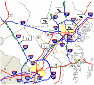
Figure 5.4: Detector Map for Minnesota Data 101
Figure 6.1: Results Illustration of lsh (up) and sqr (down) for UK 4762a, Oct 02, 1996 137
Figure 6.2: Results Illustration of lsh (up) and sqr (down) for UK 6951a, Feb 1, 2002 138
Figure 6.3: Results Illustration of lsh (up) and sqr (down) for MD 9b, Jan 16, 2004 139
Figure 6.4: Results Illustration of lsh (up) and sqr (down) for MN 882, Jul 29, 2000 140
Figure 6.5: Results Illustration of lsh (up) and sqr (down) for MN 882, Mar 30, 2004 141
Figure 6.6: Results Illustration of lsh (up) and sqr (down) for WS ES_130D_MS_Stn, Sep 9,
2004 142
Figure 6.7: Outlier Detection Illustration for Choice A (up) and Choice B (down) 171
Figure 6.8: Full System Illustration for UK 4762a, Oct 02, 1996 181
Figure 6.9: Full System Illustration for UK 6951a, Feb 1, 2002 181
Figure 6.10: Full System Illustration for MD 9b, Jan 16, 2004 182
Figure 6.11: Full System Illustration for MN 882, Jul 29, 2000 182
Figure 6.12: Full System Illustration for MN 882, Mar 30, 2004 183
Figure A.1: Sample ACF for UK 4762b, 1996 199
Figure A.2: Sample ACF for UK 4680b, 2002 199
Figure A.3: Sample ACF for MD 2a, 2004 200
Figure A.4: Sample ACF for MN 60, 2000 200
Figure A.5: Sample ACF for MN 737, 2004 201
Figure A.6: Sample ACF for WS ES_130D_MN_Stn, 2004 201
Figure G.1: Sensitivity of MAE to Forgetting Factor for Short-Term Kalman Filter 262
Figure G.2: Sensitivity of MAPE to Forgetting Factor for Short-Term Kalman Filter 262
Figure G.3: Sensitivity of RMSE to Forgetting Factor for Short-Term Kalman Filter 263
Figure G.4: Sensitivity of RMSEP to Forgetting Factor for Short-Term Kalman Filter 263
Figure G.5: Sensitivity of LPI to Forgetting Factor for Short-Term Kalman Filter 264
Figure G.6: Sensitivity of Prediction Confidence Interval Kickoff Percentage for All Traffic
Level to Forgetting Factor for GARCH filter 264
Figure G.7: Sensitivity of MAE to Seasonal Exponential Smoothing Parameter 265
Figure G.8: Sensitivity of MAPE to Seasonal Exponential Smoothing Parameter 265
Figure G.9: Sensitivity of RMSE to Seasonal Exponential Smoothing Parameter 266
Figure G.10: Sensitivity of RMSEP to Seasonal Exponential Smoothing Parameter 266
Figure G.11: Sensitivity of Prediction Confidence Interval Kickoff Percentage for All Traffic
Levels to Seasonal Exponential Smoothing Parameter 267
Figure H.1: Results of UK 4762a, Oct 02, 1996 (lambda = 1) 268
Figure H.2: Prediction CI from Different Lambda for UK 4762a, Oct 02, 1996 268
Figure H.3: Results of UK 6951a, Feb 01, 2002 (lambda = 1) 269
Figure H.4: Prediction CI from Different Lambda for UK 6951a, Feb 01, 2002 269
Figure I.2: Sensitivity of MAPE to AKF Algorithm Memory 270
Figure I.3: Sensitivity of RMSE to AKF Algorithm Memory 271
Figure I.4: Sensitivity of RMSEP to AKF Algorithm Memory 271
Figure I.5: Sensitivity of LPI to AKF Algorithm Memory 272
Figure I.6: Sensitivity of Prediction Confidence Interval Kickoff Percentage for All Traffic
LIST OF ABBREVIATIONS
ACF AutoCorrelation Function
AIC Akaike Information Criterion
AKF Adaptive Kalman Filter
AO Additive Outlier
AR AutoRegressive
ARCH AutoRegressive Conditional Heteroscedasticity
ARIMA AutoRegressive Integrated Moving Average
ARMA AutoRegressive Moving Average
ATIS Advanced Traveler Information System
ATMS Advanced Traffic Management System
CI Confidence Interval
CLS Conditional Least Square
CT Cell Transmission
DA Data Augmentation
DOT Department Of Transportation
DSPM Discrete State Propagation Model
EM Expectation Maximization
ERLS Extended Recursive Least Square
FHWA Federal HighWay Administration
FWRBFNN Fuzzy Wavelet Radial Basis Function Neural Network
GARCH Generalized AutoRegressive Conditional Heteroscedasticity
HCM Highway Capacity Manual
HOV High Occupancy Vehicle
HW Holt-Winter
IO Innovational Outlier
IMA Integrated Moving Average
ITS Intelligent Transportation Systems
K-NN K-Nearest Neighbor
KARIMA Kohonen maps with AutoRegressive Integrated Moving Average
KF Kalman Filter
LCT Lagged Cell Transmission
LMS Least Mean Square
LPI Leeds Performance Index
LS Level Shift
LSD Least Significance Difference
LWR Lighthill – Whitham – Richards
MAE Mean Absolute Error
MAPE Mean Absolute Percentage Error
MIDAS Motorway Incident Detection and Automatic Signaling
ML Maximum Likelihood
MLE Maximum Likelihood Estimation
PACF Partial AutoCorrelation Function
RLS Recursive Least Square
RMSEP Root Mean Square Error Proportional
SACF Sample AutoCorrelation Function
SARIMA Seasonal Autoregressive Integrated Moving Average
SBC Schwarz Bayesian Criterion
SCAT Sydney Coordinated Adaptive Traffic system
SCOOT Split Cycle Offset Optimization Technique system
STARIMA Space-Time AutoRegressive Integrated Moving Average
TC Temporary Change
TDAD Traffic Data And Distribution
TMC Traffic Management Center
ULS Unconditional Least Square
UTCS Urban Traffic Control System
CHAPTER 1
BACKGROUND, MOTIVATION, AND ORGANIZATION
1.1
B
ACKGROUNDCongestion and its side effects such as environmental pollution, safety degradation,
mobility deterioration, etc. have been great concerns for both the public and the
transportation engineers in developed countries. Congestion, defined as traffic demand
exceeding traffic capacity, occurs both in urban arterials and freeway systems. Of particular
interest are the freeway systems within metropolitan areas where congestion often occurs in
peak hours when the traffic demand is more compact and intense. A well-known
phenomenon of congestion is traffic break down, or stop-and-go traffic, which, ironically,
reduces the capacity when it is most urgently needed and causes a large amount of delay.
Due to the limitation in constructing new road in already crowded metropolitan areas,
freeway management has been an important alternative to improve freeway operations.
According to the Freeway Management and Operations Handbook (FHWA 2003), freeway
management is defined as “the implementation of policies, strategies and technologies to
improve freeway performance” with its over-riding objectives to “minimize congestion
(and its side effects), improve safety, enhance overall mobility, and provide support to other
agencies during emergencies”. Major freeway management techniques identified in the
handbook include lane management, ramp management, high occupancy vehicle (HOV)
ramp metering has been regarded as “the most direct and efficient way to control and
upgrade freeway traffic” (Parageorgiou et al. 2003).
Proactive traffic control systems call for an ability to anticipate the traffic condition in
the near future, yielding so called short-term traffic forecasting problem. Freeway
management systems can be proactive or reactive according to the traffic condition based
upon which the control strategies are developed. If the real time data indicating current
traffic condition are utilized, the resultant control system is at most reactive;
correspondingly, if forecasts indicating the near future traffic condition are utilized, the
resultant control system is proactive. Obviously, proactive traffic control actions have a
better chance of success if the future traffic conditions are accurately predicted. Thus, to
make the most from the freeway management systems, predictive ability has been
identified as one of the major challenges for advanced traffic management system (ATMS)
and advanced traveler information system (ATIS), as is also pointed out in the Ten Year ITS
program plan (ITS America 2002). Specifically, for ramp metering control, current
strategies in practice are at most reactive, using either historical traffic information
(pre-timed control) or real-time traffic measurements (local or coordinated
traffic-responsive control) (Chu et al. 2004). From a proactive point of view, a
comprehensive optimal control concept was discussed in (Parageorgiou and Kotsalos, 2002)
and (Parageorgiou et al. 2003), requiring an explicit consideration of “demand predictions
algorithm has also been recognized in (Jacobson et al. 1989).
Recent advancement in the analysis of freeway traffic operation data also provides a
firm support for pursuing accurate prediction capability as a means to improve the
effectiveness of freeway control systems. A two regime, discontinuous model of freeway
traffic flow as is argued in (Payne 1984) has been implicitly recognized in freeway control
systems, especially for ramp metering algorithms. In this two regime model, freeway traffic
condition is described as either being in a non-congestion state, a congestion state, or a
connecting transient state. When congestion occurs, the traffic state will switch from
non-congestion to congestion through a short transient state. Should the transient state be
detected or anticipated, control measures can be applied and be expected to prevent or
delay the occurrence of the congestion. The same argument is also presented in the
Freeway Management and Operations Handbook (FHWA 2003).
Two aspects are inherently implied in a forecasting problem, i.e., the accuracy of the
forecast and its credibility, indicated by the prediction confidence interval. A plausible
forecasting system is expected to provide the answers to both of the aspects. The accuracy
of the forecast enables the control system relying on that to work appropriately while the
credibility will shed light on the uncertainty of the adopted control strategy. Actually in
current customer-oriented traffic system, the knowledge of the uncertainty is an essential
attribute of mobility. Unfortunately, so far the research on forecast confidence interval is
Various control methods in a freeway control system call for a corresponding traffic
forecasting framework. Intelligent Transportation Systems (ITS), the application of
advanced technology in transportation and an important enabler for freeway management
systems, helps to maintain an information supply chain in a freeway management system.
In this information supply chain, different end users have different requirements for the
forecasting algorithm. For example, commuters desire a forecast of travel time, rather than
a forecast of flow rate; however, the forecast of travel time might not be readily applicable
to a proactive ramp metering algorithm. In addition to commuters, other end users might be
traffic engineers, freeway control algorithms, or other decision making procedures. Thus, in
order to address the user specific requirements, clarification of the short-term traffic
forecasting attributes will be the first step of developing a forecasting strategy.
1.2
M
OTIVATIONThis research aimed to develop a robust online forecasting strategy based on previous
research in order to provide the anticipatory ability required by a proactive freeway
management and control system. This strategy can forecast traffic condition in the near
future and generate its confidence interval based on real time freeway operation data.
This strategy can be implemented at traffic management centers (TMC) to facilitate the
operation of the freeway systems in the US or other countries, such as the motorway
freeway control strategies, such as ramp metering algorithms, to provide traffic condition
forecasts for the purpose of a better control. Compared to previous work, this effort
explicitly separates the forecasting strategy development into two major steps: the batch
mode investigation of traffic dynamics and the online implementation of the identified
batch mode traffic dynamics model.
1.3
T
HESISO
RGANIZATIONThis research intends to develop an online traffic condition forecasting system. In all,
seven chapters including this introductory chapter are presented and the organization of the
dissertation is summarized below.
Chapter 2 discusses the research problem, including the general short-term traffic
forecasting problem definition, attributes of “ideal” forecasting methods, and the
specifications of the proposed forecasting system.
Chapter 3 presents a literature review of previous research on short-term traffic
forecasting, including the classification of the forecasting methods and the discussion of the
methodological highlights of each method. Afterwards, robust forecasting is reviewed. A
comparison table summarizes the review.
Chapter 4 describes the methodology for developing the online forecasting system,
Chapter 5 provides a description of the real traffic condition data utilized in this work.
Chapter 6 performs the development and testing of the online forecasting system,
including experimental design, traffic dynamics investigation, online system
implementation and testing.
Chapter 7 summarizes the research findings and presents the recommendations for
CHAPTER 2
PROBLEM STATEMENT
This chapter presents the problem to be addressed in this study. Firstly, the general
short-term traffic forecasting problem and the associated attributes are defined and
discussed. Secondly, the characteristics of “ideal” traffic condition forecasting algorithms
are discussed for the purpose of algorithm evaluation. Finally, the specifications of the
forecasting algorithm proposed in this work are articulated in compliance with the previous
discussions on the general forecasting algorithm characteristics.
2.1
G
ENERALS
HORT-T
ERMT
RAFFICF
ORECASTINGP
ROBLEMD
EFINITIONInductive loop detectors are the most widely applied traffic monitoring devices used in
freeway management systems. A typical three lane freeway section instrumented with
inductive loop detectors is demonstrated in Figure 2.1. In this layout, detectors are
distributed spatially across each lane and the three adjacent detectors at a specific location
form a detection station, e.g., station i. For each time interval indexed by time stamp t,
each loop detector produces a set of traffic data indicating traffic conditions for this time
interval, typically including flow rate, occupancy, and speed if a speed trap with two
closely-spaced detectors is used. Data from three detectors form the station data,
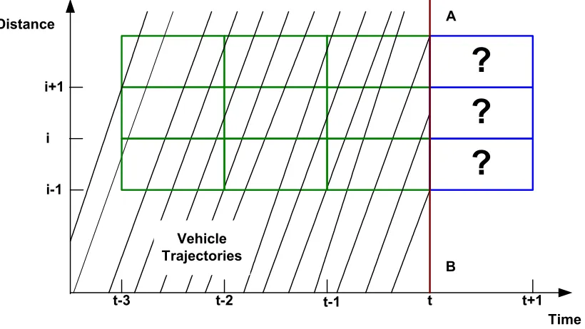
corresponding to the aggregation of a rectangle to the left of line AB in Figure 2.2. An
important point worth mentioning is that the size of these rectangles is closely related to the
historical traffic condition database
{
Ω( )
t , t =1,2,3,...}
. Clearly, the historical trafficcondition database is spatial and temporal in nature.
Inductive Loop Detector Traffic Direction
i-1 i i+1
li-1 li
Figure 2.1: Typical Layout of an Instrumented Freeway Section
i i+1
t-1 t t+1
Distance
Time i-1
t-2
A
B Vehicle
Trajectories
t-3
?
?
?
The general traffic condition prediction can be stated as: Given a historical traffic
condition database up to current time interval indexed by time stamp t , i.e.,
( )
{
Ωt , t =1,2,3,...,t}
, find the traffic condition set{
Ω( )
t ,t =t+1,t+2,...,t+k}
, where k isthe prediction horizon with k =1 for the one-step-ahead prediction. In Figure 2.2, the historical traffic condition database is represented as the aggregation of traffic condition
within each rectangle to the left of the line AB and the forecasts at different locations are
represented as the aggregation of traffic condition within the rectangles with question
marks that are to the right of the line AB.
In the short-term traffic forecasting problem, although by-lane traffic condition data
are available and by-lane forecasting is feasible, all the previous work (to the best
knowledge of the author) and this work included intend to forecast traffic condition at a
station. Note that site is also used in the literature indicating a station as defined previously.
In this dissertation, “site” and “station” are used interchangeably hereafter. One point need
to point out is that in order for a fair comparison between locations with different number
of lanes, the traffic operation data for each station is normalized by the number of lanes. In
the following analyses, unless specifically pointed out, the traffic data utilized are after the
normalization.
There are many specifications which are necessary to characterize a traffic forecasting
(1) Prediction Variable
According to the number of prediction variables employed, a forecasting algorithm can
be univariate or multivariate. Univariate processing can also be termed as point forecasting,
which make use of only one traffic variable at a single station. For example, traffic flow
rate is typically used for ramp metering. Although less information is utilized, univariate
processing is still promising in that relative simple forecasting methods with satisfying
accuracy can be formulated, especially for forecasting at longer time intervals where traffic
state propagation can be captured by using traffic data from a single station. Compared
with univariate processing, more information, for example, traffic data from surrounding
sites and/or additional traffic variables, is applied in multivariate forecasting methods. A
recent multivariate application was developed in Guin (2004), in which 20-second traffic
flow rates are forecasted using the upstream and downstream station data for the purpose of
automatic incident detection. The selection of the prediction variable is closely related to
the forecasting horizon, which is discussed in the subsequent section. For forecasting at a
higher time scale, the calibration of the relationship between these traffic variables is a
complicated task, although multivariate processing seems appealing. Other concerns such
as time varying cross-correlation are also to be considered for multivariate processing.
(2) Time Scale
algorithm can be microscopic or macroscopic. The typical time scales for microscopic
processing are 20-second, 30-second, or 1-minute. Microscopic processing is necessary for
time-critical applications such as incident detection. The most widely used time scale for
macroscopic processing is 15-minute conforming to the convention of Highway Capacity
Manual (HCM). Other intervals such as 5-minute, 10-minute are also presented in the
literature. Macroscopic processing relies on the aggregated traffic condition data, and
compared with microscopic processing, macroscopic processing can provide the traffic
condition prediction into a further future.
The selection of traffic forecasting variable and its aggregation time scale has a close
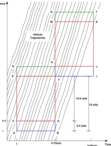
relationship with traffic state propagation. Figure 2.3 illustrates a hypothetical freeway
section with adjacent detection stations i and i+1 at a spacing of 0.5 mile. Assume the traffic on this section has an almost stationary state with a space mean speed 60 mile per
hour. So within 15 minutes, a traffic state can propagate to 60 4=15 miles downstream
further. For station i, the traffic condition from t to t+15minutescan be represented by the aggregation of vehicles crossing the zone ABEF. Similarly, for station i+1, the traffic condition from t to t+15mincan be represented by the aggregation of vehicles crossing the zone CDGH. Using assumed traffic stream speed and detection station spacing, the
overlay between these two zones, i.e., zone CDEF, has approximately a length of
5 . 14 5 . 0
15− = miles; in other words, around
(
14.515.5)
×100%=93.5%of the 15-minute15-minute univariate flow rate at a single station as the forecasting variable in this work.
For this nearly stationary traffic, these condition zones for time interval from t to
minutes 15
+
t will propagate to zones for time interval from t+15minutes to
minutes 30
+
t , i.e., ABEF to FIKM, CDGH to HJLN, and overlap CDEF to HJKM. For real traffic, the propagation of traffic condition is governed by the traffic dynamics.
Therefore, the problem of short-term traffic forecasting is to propagate current traffic
condition to forecasting horizon according to pre-identified traffic dynamics. Intuitively,
this pre-identified traffic dynamics model will in a sense dominate the performance of the
i i+1
t t+15min
t+30min Distance
Time 14.5 mile
0.5 mile
15 mile Vehicle
Trajectories
A B
C D
E
F G
H
I J K L
M N
Figure 2.3: Traffic State Propagation at 15-minute Interval
It can be deduced that as the aggregation interval decreases, the traffic overlap between
station data into the forecasting strategy in order to improve the forecast. This is often the
case for microscopic level processing. The most recent development to this end is the
discrete state propagation model developed in Guin (2004) based on a revision of Lagged
Cell Transmission Model (Daganzo 1999).
(3) Algorithm Memory
A forecasting algorithm can be implemented as a batch mode process or a recursive
process according to the size of algorithm memory. In batch mode processing, a finite set of
historical traffic data is retained in the forecasting system. With the incoming traffic stream,
the historical database is updated and the forecast is produced based on the entire historical
database, causing a heavy computational burden. To ensure the forecasting quality, the
historical database should be routinely maintained. Compared with batch mode processing,
recursive processing has a smaller algorithm memory and the forecast is produced based on
the predefined recursion equation when new traffic data are available. Due to the reduced
algorithm memory, recursive processing has a reduced amount of computation and thus a
higher computational performance. Batch mode processing would seem to promise more
accurate forecasts; however, it is not suitable for online traffic applications where traffic
data are collected in stream. Therefore, recursive processing has a greater potential in time
critical applications as is often the case in Intelligent Transportation Systems. For example,
the timely detection of an incident will greatly reduce its negative effects on traffic
(4) Adaptability
A short-term traffic forecasting method can be either adaptive or non-adaptive
depending on the way the algorithm responds to the incoming traffic data. Traffic is
dynamic in nature; thus, the traffic condition data stream arising from the traffic is dynamic.
In adaptive processing, the incoming traffic data is first used to update the forecasting
system; then the forecast is produced based on the updated forecasting system. Adaptive
processing is promising in that it provides a mechanism for learning the evolution of the
traffic process. Compared with adaptive processing, non-adaptive processing cannot adapt
to the incoming of traffic stream and has a high chance of deviating from the real traffic
condition state over time (Ahmed 1989). For example, most heuristic forecasting methods
are non-adaptive forecasting methods. Under these circumstances, a restart of the
forecasting algorithm might be needed to reflect the current traffic conditions. The
adaptability is further discussed in the succeeding section.
2.2
I
DEALS
HORT-T
ERMT
RAFFICF
ORECASTINGM
ETHODSAlthough different forecasting algorithms within the forecasting framework have
different evaluation criteria, theoretically, “ideal” traffic forecasting algorithms share some
common characteristics which are discussed below.
Competencies for a short-term traffic forecasting algorithm include at least two aspects:
the generation of satisfactory forecasts to meet the specific requirements and the provision
of the credibility of the forecast. Actually these two aspects constitute the basic essential
requirements for any forecasting structure. Failure in providing of either one will degrade
the usefulness of the forecasting algorithm.
(2) Implementation Efficiency or Transferability
Implementation efficiency means that a short-term traffic forecasting system should be
easily implemented across various locations, or a forecasting algorithm would be “plug and
play” in nature. This characteristic describes the transferability of a forecasting method. In
this regard, a forecasting algorithm should first be easily implemented into existing traffic
condition surveillance and control systems without requiring much revision of the current
system. Secondly, the new component should work without massive manual calibration to
capture the location specific attributes through, for example, a test run within a short period
of time. To summarize, the involvement of the location specific parameters and the way
these parameters are calibrated or identified are two of the most important factors affecting
the forecasting system transferability.
(3) Computation Efficiency
In a real freeway operation situation, traffic condition data will be continuously
control. Under this situation, a forecasting algorithm, as a preprocessor before succeeding
control strategies, is expected to generate the forecast with the least possible computational
burden in order to guarantee a fast response. Therefore, the forecasting algorithm in a
recursive form with limited algorithm memory is suitable to produce the forecast only
using the current traffic data with all the previous information encapsulated in the recursion
equation.
(4) Adaptability
A forecasting algorithm is expected to be self-tuning to the incoming data stream.
Obviously, traffic is far from stationary. For example, traffic condition data may have
pronounced patterns such as a weekly pattern and/or a daily pattern, which perturb the level
of traffic during different times of the day and different days of the week. Additionally,
traffic also suffers from exogenous disturbances, such as weather changes, holidays, special
events, etc., all of which call for a learning scheme in the forecasting algorithm to adapt to
these temporary changes of traffic condition.
The adaptability of the forecasting system can embrace two different strategies, i.e., (1)
updating the system structure indicated by the system parameters and/or the historical
databases, and (2) switching the forecast generation equation based on changes in traffic
dynamics. The first strategy is clear in that the forecasting system state indicated by system
when the forecasting system has a set of forecast equations. A typical example is the
discrete state propagation model in Guin (2004) where a set of forecasting equations were
established for different traffic regimes and then selected according to traffic dynamics
changes.
(5) Robustness
Robustness is an important factor in enabling normal operation of a forecasting system.
Due to the somewhat unavoidable errors in the traffic condition data collection system,
suspect data and erroneous data are common in traffic condition databases. A robust
forecasting strategy should only respond to the “good” data with “bad” data handled or
ignored. Missing values and outliers are two of the most widely recognized difficulties in
developing a forecasting strategy. Missing values have been regarded as a common
attribute of ITS traffic operations data due to the continuous nature of the traffic monitoring
equipment (Turner 2001). Missing value imputation has been studied extensively and
heuristic approaches and statistical approaches have been developed. Outliers, observations
that are significantly different from other observations, are generated by an unknown
process which is different from the process under study. A most common source of outliers
might be traffic incidents that perturb the traffic dynamics temporarily. So far, there is
limited research on outlier detection on traffic condition data forecasting except for
Williams (1999). Actions should be taken for a robust forecasting strategy to detect and
Adaptability and robustness are closely related in that both attributes require the
forecasting system to make a response when something unusual happens. Obviously, the
characters of the unusual events, or exogenous disturbances, are important for a proper
differentiation of adaptability and robustness. One important attribute of relevance is
whether or not the unusual event changes the travel pattern. For example, a special event
might temporarily change the travel pattern for days. In this case, a forecasting algorithm
might need to capture the pattern change and make forecasts that are consistent with the
changed pattern. The forecasting algorithm will adapt back to normal again when the event
is over. However, for a traffic incident, supposing this incident information is not available
to the public, the travel pattern will remain the same and traffic will return to normal when
the incident is cleared. In this case, the forecasting algorithm might need to detect the
disturbance and ignore it. One rough condition for testing the travel pattern change might
be the duration of the effect of the exogenous events. There is also an urgent need for a
forecasting framework, within which the proper responses of a forecasting algorithm for
various traffic control and management scenarios need be clearly defined. In other words,
the forecasting system must be tailored to its real application purposes.
2.3
S
PECIFICATIONS OFP
ROPOSEDA
LGORITHM INT
HISS
TUDYThe traffic condition forecasting strategy to be developed in this research has the
(1) Univariate Traffic Flow Rate at 15-minute Level
This forecasting strategy uses 15-minute traffic flow rate at a single station as the
forecasting variable. The forecasted value will be the 15-minute traffic flow rate at the
same station for the next 15-minute. This choice is supported by the freeway traffic state
propagation demonstration illustrated in Figure 2.3.
It is important to emphasize that the 15-minute interval selected for this study is just a
representative of a spectrum of aggregation intervals. As discussed previously, the decrease
in the time scale calls for the incorporation of temporal and spatial information, yielding a
cutoff time interval, above which there is a spectrum of intervals that the proposed
univariate forecasting method can be applied to. Therefore, the proposed methodology is
expected to work for similar aggregation intervals, say 20-minute and/or 10-minute, within
this spectrum, although no detailed investigation will be performed in this study to
determine the cutoff interval. In addition, this strategy can also be extended to model other
traffic condition variables such as occupancy and/or speed.
(2) Sound Traffic Dynamics Investigation
The development of the forecasting strategy will follow two stages. Firstly, the
dynamics of traffic condition series (15-minute flow rate series in this study) will be
investigated in batch mode to capture the inner regularity embedded in the data. The first
(conditional variance) of the series will be modeled. Secondly, the batch mode modeling
results will be converted into an online version using the techniques of seasonal
exponential smoothing and Kalman filter theory.
(3) Joint Production of Forecasts and Forecast Confidence Intervals
The forecasts and the associated forecast confidence intervals are jointly produced in
this online forecasting system. The forecasts are produced using the first order conditional
moment model and the forecast confidence intervals are produced using the second order
conditional moment model. The first order conditional moment is modeled as the Seasonal
Integrated Autoregressive Moving Average (SARIMA) process, which is implemented
using the technique of seasonal exponential smoothing and Kalman filter. The modeling of
the first conditional moment has been conducted in the literature and Williams (1999) is the
most up-to-date work where a sound theoretical justification of the SARIMA model was
firstly recognized based on the Wold Decomposition Theorem. The second order
conditional moment is modeled as the Generalized Autoregressive Conditional
Heteroscedasticity (GARCH) process, which is implemented by a Kalman filter using the
squared forecasting error as inputs.
(4) Transferability across Locations
This forecasting strategy is expected to possess an ability of learning the
locations without massive manual calibration. In this study, the system transferability will
be demonstrated using real traffic data from various regions.
(5) Recursive Processing with Reduced Computational Burden
This forecasting strategy is based on the techniques of seasonal exponential smoothing
and Kalman filter, both of which are recursive in nature. Therefore, the forecasting
algorithm has limited algorithm memory and the computational burden is greatly reduced
since it only responds to incoming traffic condition data with previous traffic information
encapsulated in the current system state.
(6) Adaptability
This online forecasting strategy employs Kalman filter, which itself can adapt to
changing traffic dynamics. Efforts to apply an adaptive Kalman filter will be conducted and
tested to fine-tune the Kalman filter. The system adaptability will be investigated using real
traffic operations data.
(7) Robustness
This forecasting strategy has the ability to handle missing values and detect outliers to
conduct robust forecasting. Unlike the outlier detection in Williams (1999), where the
constant process variance was implicitly assumed, time varying conditional variance is
occurrence of missing values and the response of the system to outliers will be investigated.
This forecasting strategy can be implemented at a TMC, and the forecasting results can
be directly fed into the development of traffic control measures. The end users of this
strategy are professional traffic engineers who can respond to the forecast of traffic flow
rate and intermittent freeway control systems that make use of the forecast in the control
measurement development. Furthermore, the quantified uncertainty indicated by the time
varying prediction confidence intervals can be explored in succeeding research for the
purpose of enhancing the mobility of transportation systems.
2.4
S
UMMARYDifferent uses of the traffic condition forecast call for different treatments of the
forecasting system. This research is to establish an online short-term univariate traffic
condition prediction system incorporating online missing value imputation and outlier
detection. The algorithm uses 15-minute traffic flow rates as a representative time interval
and is intended to provide the proactive ability for advanced traffic control. The prediction
CHAPTER 3
LITERATURE REVIEW
In this chapter, a review of the short-term traffic forecasting methods is presented to
reveal the connection and improvement of the proposed method over previous efforts.
Firstly, the short-term traffic forecasting methods are classified into seven categories.
Detailed discussions on the methodological highlights and the applications of each method
are provided in the subsequent section. A concise review on the traffic condition data
validation which is closely related to robust forecasting is presented afterwards. The
chapter concludes with a comparison table summarizing the forecasting methods review.
3.1
C
LASSIFICATION OFF
ORECASTINGM
ETHODSA variety of short-term traffic forecasting methods have been developed since the start
of the research several decades ago. These methods can be generally classified into seven
categories discussed below.
3.1.1 Heuristic Methods
The efforts until early 1980s were on the heuristic methods, or ad hoc methods,
including random walk, historical average, informed historical average, and UTCS
predictors. The historical traffic pattern and current traffic condition are two important
components in constructing these methods. The heuristic methods share a common
arbitrary utilization of traffic data, where personnel knowledge and engineering judgment
are crucial for a successful deployment. Moreover, none of these methods has the ability of
adapting to the changing traffic condition (Stephanedes et al. 1981).
3.1.2 Linear Statistical Methods
Researches in 1980s and 1990s saw an adoption of the linear statistical theory. The
most widely tested method is the univariate Box-Jenkins time series method in time domain.
This method assumes a linear combination of past observations and forecasting errors can
capture the traffic dynamics, thereby satisfactory forecasts can be constructed. The method
essence is to capture the linear correlation structure embedded in the traffic condition series.
Correspondingly, in frequency domain, based on the inherent assumption of a stable daily
traffic pattern, the spectral representation method using the orthogonal series
decomposition also falls into this category. Multivariate time series models belong to this
category, too, in that although complicated in form, it is still the linear structure of the
multivariate traffic condition series to be modeled. Three multivariate time series methods
were developed, i.e., vector ARIMA (VARIMA) model, space-time ARIMA (STARIMA)
model, and ARIMAX model.
Exponential smoothing also falls into this category due to its equivalent reformulation
to ARIMA model (McKenzie 1984). In exponential smoothing, the traffic condition data
exponential smoothing generally works well in practice (Chatfield et al. 1988).
All these methods are constructed based on prescribed parametric models, recognizing
the linear traffic structure. However, should no online estimation procedure be incorporated,
these methods cannot provide the ability of adaptation.
3.1.3 Nonlinear Methods
Based on the recognition of the seemingly nonlinear/chaotic nature of the traffic,
nonlinear methods have been investigated extensively since 1990s with an expectation that
an appropriately designed nonlinear structure can simulate the traffic dynamics and
generate a good forecast. The neural network method from artificial intelligence and the
non-parametric method from nonlinear statistical theory are two major approaches. The
neural network model applies interconnected and layered neurons to model the nonlinearity
in traffic data and a variety of neural network models have been devised and tested. The
non-parametric method embraces a set of techniques for curve estimation without making
strong assumptions on the true curve. K-nearest neighbor (K-NN), kernel smoothing, and
local linear regression are three methods that have been applied to traffic forecasting. In
these methods, localized sets of traffic condition data are selected and utilized to generate
the forecasts. It is worthwhile to note that the bandwidth or span denoting the size of the set
is of central role in these methods (Altman 1992).
on which the ability of adaptation is induced. The learning strategy generally requires either
a historical traffic database or a localized set with arbitrary size, both of which might
impose certain negative effects. For example, better forecasting accuracy and learning
efficiency requires a sizable historical database, which will increase the computational
burden.
Recent researches conducted on the traffic state transition using the loop detector data
undermined the strength of the nonlinear approach. It was shown that the traffic dynamics
can be best modeled using the simple first order continuum theory and complicated traffic
phenomena, even the most mysterious one as traffic hysterics, can be well explained.
Daganzo (2002) presented a summary of these studies. These researches suggested a simple
linear intrinsic regularity in the traffic dynamics; thus linear theory based methods are
expected to yield better results than those based on nonlinear theory.
3.1.4 Hybrid Methods
Hybrid methods include the combination of methods and the combination of forecasts.
The combination of methods is to construct a new forecasting method by combining two or
more forecasting methods. Efforts were made to combine the linear methods and nonlinear
methods where a nonlinear method is applied to construct clusters of traffic condition data
and a linear method is applied to each cluster to produce the forecasts. Typical methods are
disadvantage of destroying the possible inner mechanism across time in the traffic
condition series through clustering operation. For example, the data close to the edge of
each cluster might not be sharply different from each other while the forecasting strategies
are totally different. The combination of the forecasts, termed by prediction combination in
this study, is to produce a forecast by combining the forecasts of the same quantity from
two or more individual forecasting methods based on the premise that the combination of
the forecasts is almost always better than selecting a single “best” forecast.
Intuitively, the characters of a hybrid method are determined partly by the characters of
involved individual forecasting method. For example, if a neural network is applied, the
hybrid method might inherit a disadvantage of heavy computational burden, while the
advantage of adaptation might also be transferred to the hybrid method as well. In addition,
the hybrid methods generally have complicated structures, restricting the cross location
implementation.
3.1.5 Traffic Flow Theory Based Methods
Traffic flow theory that describes the law of traffic dynamics provides a natural
forecasting method. So far the field of traffic flow theory includes the simple first order
continuum theory (Lighthill and Whitham 1955, Richard 1956) and the higher order
continuum theory (Whitham 1974 and Payne 1979). Due to the recent researches on traffic
order theory (Daganzo 2002). Discretized versions of the first order continuum model, e.g.
Cell Transmission Model (Daganzo 1994, 1995) and Lagged Cell Transmission Model
(Daganzo 1999), are good candidates for constructing forecasting methods. Discrete state
propagation model (DSPM) by Guin (2004) was developed based on a revision of the LCT
model for the purpose of automatic incident detection.
Traffic flow theory based method is natural to incorporate multiple traffic variables
into the forecasting system. However, as is discussed in the traffic state propagation, the
forecasting horizon is generally at low level for this approach.
3.1.6 Adaptive Forecasting Methods
The non-stationary traffic dynamics calls for an adaptive forecasting strategy and the
awareness of bringing adaptability into traffic forecasting system can be traced back to the
early stages of the research (Stephanedes et al. 1981).
Adaptive filters adopted from other disciplines, mainly digital signal processing and
dynamic system control, are the most widely applied adaptive forecasting methods. The
adopted adaptive filters include recursive least square (RLS), Kalman filter, generalized
linear model (GLM), and least mean square (LMS) filters. These methods are promising in
imparting a self-adjusting ability into the forecasting system; however, contrary to the
discussion in Stephanedes et al. (1981) that forecasting method should be built upon solid
autoregressive models for the traffic dynamics based on personal judgment or preference.
3.1.7 Other Methods
This category includes traffic forecasting methods which cannot be clearly classified
into previous categories for the purpose of completeness. A typical method is Gaussian
Maximum Likelihood Formulation in Lin (2001) and Lin et al. (2002) based on the
investigation of the traffic level and the traffic level increment.
3.2
M
ETHODOLOGICALH
IGHLIGHTS OFF
ORECASTINGM
ETHODSThis section describes the methodological highlights of the traffic forecasting methods.
Applications are presented and references provided for interested readers.
3.2.1 Random Walk
Random walk model is the simplest forecasting method which assumes traffic
condition for the next time interval is the same as that in the previous one, i.e., Vˆt+1=Vt, where Vˆt+1 is the forecast for time interval t+1 and Vt is the traffic condition for time interval t. No historical traffic pattern is utilized herein. Without parameters in the
forecasting system, random walk model is easily to be implemented across locations and is
implicitly applied in any system that responds to the current traffic conditions, such as the
3.2.2 Historical Average
Compared with the random walk model that ignores the historical pattern, historical
average takes the forecast as an average of all the observations for the same time interval of
the day. Obviously, totally ignoring current traffic condition, it cannot respond to the time
varying traffic condition and is not appropriate for dynamic traffic control. Additionally,
although historical pattern can be extracted by this method, the exponential smoothing is a
more powerful tool in capturing the historical pattern by assigning an exponential
weighting scheme to historical traffic observations. Simple in form, the historical average
method is easy to be implemented as is the random walk model.
3.2.3 Informed Historical Average
Informed historical average aims to combine the historical pattern and the current
traffic condition in order to improve the forecasting performance, and it is also easy to be
implemented as no parameters are involved in the forecasting system. As is pointed out in
Williams (1999), such a combination is still “classified as simple if it requires no fitting or
fine-tuning to site specific characteristics”.
An informed historical average method was proposed in the ALI-SCOUT system for
travel time forecasting (Kaysi et al. 1993). This method firstly computes the ratio of the
historical travel time on a specific link to the current travel time; then the ratio is used
remedy the random walk assumption, Kutsopoulos and Xu (1993) suggested the use of the
information discounting, a strategy to adjust or penalize the current link travel time
according to the amount of the value and the standard error of the historical travel time on
the same link.
3.2.4 UTCS Predictor
Urban Traffic Control System was developed for the testing of advanced network
control methods and strategies. Three generations of predictors have been developed. In the
first generation UTCS, the forecast relied heavily on the historical data; the second
generation predictor, i.e., UTCS-2, utilized both historical data and current data; and the
third generation predictor, i.e., UTCS-3, generated prediction according to merely current
data. Though having complicated forms, these methods are still heuristic because of the
arbitrary treatment of the traffic data and the lack of rigorous justification. A
comprehensive comparison conducted in Stephanedes et al. (1981) showed that UTCS-2
had the best performance in the sense of mean square error and mean absolute error when
compared with random walk, historical average, and UTCS-3. Since there are some
parameters involved in the forecasting system, the parameter calibration required for
appropriate deployments will restrict the transferability.
3.2.5 Univariate Box-Jenkins Method
of adaptability and rigorous justification), attention was paid to the investigation of traffic
dynamics in order to find a better method with sound theoretical foundation. The
recognition of traffic process to be a point process leaded to the adoption of the univariate
time series modeling. Box-Jenkins approach (Box and Jenkins 1994) is the most widely
applied time series modeling method. Since this method is closely related to the proposed
forecasting method in this work, a brief description of the method is presented below. See
(Fuller 1996) for a detailed discussion.
A time series defined as
{
Xt :t∈T}
can be strictly stationary or weakly stationary. Given FX( )
⋅ as the probability distribution function and lag h, a time series is strictly stationary if(
n)
t h t h tn h(
n)
n t t
t X X t t t X X X t t t
X x x x F x x x
F , ,..., 1, 2,...,
2 1 2
1 2
1, ,..., = + , + ,..., + (3-1)
for all possible sets of t1,t2,...,tn andt1+h,t2 +h,...,tn +h. This definition states that the joint probability of any given subset of a strictly stationary time series is independent of the
lag.
A time series is weakly stationary if (1) the expected value of Xt is constant for all t; and (2) the covariance matrix of
(
Xt1,Xt2,...,Xtn)
is the same as that of(
Xt1+h,Xt2+h,...,Xtn+h)
for all finite sets(
t1,t2,...,tn)
and h. The definition of the weaklystationarity only restricts the first and second moment of the time series, and hence weakly
Theorem, a weakly stationary time series Yt defined on T =
{
0,±1,±2,...}
can be represented ast t
t X Z
Y = + , (3-2)
where Zt is a deterministic component and Xt can be modeled as an autoregressive moving average process defined as φ(B)Xt =θ(B)εt which is a subset of SARIMA process defined in the following paragraph.
For a non-stationary time series{Xt}, the Box-Jenkins approach assumes the nonstationarity can be handled by proper differencing, thus the