SEISMIC DAMAGE PROBABILITY BY GROUND MOTIONS
CONSISTENT WITH SEISMIC HAZARD
Sayaka Igarashi1, Shigehiro Sakamoto1, Yasuo Uchiyama1, Yu Yamamoto1, Akemi Nishida2, Ken Muramatsu2 and Tsuyoshi Takada3
1
Technology Center, Taisei Corporation, Kanagawa, Japan
2
Center for Computational Science and e-Systems, Japan Atomic Energy Agency, Chiba, Japan
3
Professor, Department of Architecture, The University of Tokyo, Tokyo, Japan
ABSTRACT
In the preceding study, the methodology to generate ground-motion time histories for advanced probabilistic risk assessment of nuclear power plants was proposed (Nishida et al. 2013). These ground motions are consistent with seismic hazard at reference site, and incorporate differences of seismic-source characteristics. When ground-motion time histories are required in conventional PRA, they are generated to fit to specified spectra such as uniform hazard spectra, which do not incorporate seismic-source characteristics. Moreover, they are often generated without considering the variation of spectra. Even if the variation is included, their inter-period correlations are generally assumed to be 1.0.
In this paper, the authors prepared some cases of ground-motions sets. Ground motions in all case are generated to fit to the median of the response spectra calculated from hazard-consistent ground motions, while depending on cases, they have different information about variation and inter-period correlation of response spectra. The response analyses of general RC structure and PWR building with these ground motions sets were conducted and the damage frequencies of simplified equipment system settled on the structure were compared.
As a result of damage probability evaluation of system, it is pointed that the damage probability of system affected more strongly by the variation of response spectra than the inter-period correlation of response spectra.
INTRODUCTION
After 2011 Fukushima Daiichi Nuclear Power Plant (NPP) accident, seismic probabilistic risk assessment (PRA) is regarded as the important methodology for evaluating seismic safety of NPPs quantitatively. Seismic PRA is expected to make use of sharing risk information with stakeholders and making decision on safety plan for NPPs. Therefore, the improvement of evaluation precision for PRA is now required. In the preceding study, Nishida et al. proposed an advanced PRA scheme for NPPs, where structural analyses with ground-motion time histories are conducted, and the damages of structure and equipment are evaluated based on the comparisons between their response and strength. Nishida et al. also generated ground-motion time histories for proposed scheme. The generated ground motions based on Monte Carlo simulation are consistent with seismic hazard at reference site and incorporate seismic-source uncertainties of fault model. In this study, these ground motions are called “hazard-consistent ground motions (HCGMs)”.
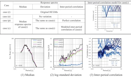
inter-period correlation for their response spectra. The cases of ground-motions set were shown in following.
࣭case(r) : hazard consistent ground motions
࣭case(n) : simulated ground motions which have no variation in response spectra
࣭case(p) : simulated ground motions which have the same variation in response spectra with case(r), where the inter-period correlation coefficient is 1.0.
࣭case(c) : simulated ground motions which the same variation with case(r) and the modelled inter-period correlation of case(r) in the response spectra.
HAZARD-CONSISTENT GROUND MOTIONS
Outline of hazard-consistent ground motions
The HCGMs objected in this study are the ground motions set of “case B” in preceding study by Takada et al. (2014), where the details of HCGMs are given. In this section, the outline of HCGMs is indicated. The HCGMs were generated for seismic sources which contribute to seismic hazard at the reference site, Oarai in Japan (Lat. 36.26°N, Lon.140.55°E). The ground-motion time histories were generated with the hybrid method of the stochastic Green’s function method and the wave integration method. In the ground-motions generation, seismic-source uncertainties are included in fault models by Monte Carlo simulation.
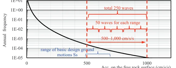
Figure 1 shows the hazard curve evaluated based on the method of HERP (2009), where the index of the seismic intensity is the maximum acceleration on the free rock surface. In the hazard evaluation, the attenuation relationship which is called “taisen spectra” proposed by Noda et al. (2002), was adopted with the variation of 0.23 (common-logarithm standard deviation). The target maximum acceleration of HCGMs was from 500 to 1,000 cm/s2, which correspond to the annual frequency from 10-4 to 10-5. A total of 250 ground motions were reproduced as HCGMs, where 50 ground motions were reproduced for each acceleration range divided into 5 with 100 cm/s2 intervals.
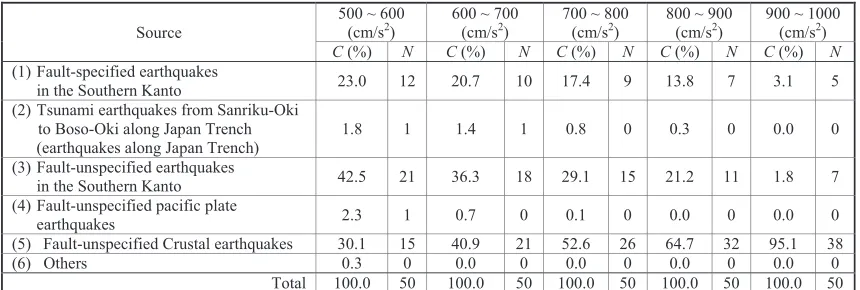
Table 1 shows the seismic sources which contribute to seismic hazard and the number of ground motions to be reproduced for each source. The seismic sources are the same with those in the preceding study by Nishida et al (2013). In the preceding study, only the aleatory uncertainties are included for source characteristics, while not only aleatory uncertainties but also epistemic uncertainties are incorporated for HCGMs in this study. Epistemic uncertainties are included for macro-scopic seismic-source characteristics by logic-tree of empirical equations, and their constants uncertainties and the micro-scopic seismic-source characteristics uncertainties are treated as aleatory uncertainties. These uncertainties are realized by Monte Carlo simulation. Figure 2 shows logic tree for macro-scopic seismic-source characteristics. Seismic moment (M0), fault area (S) and fault length (L) are regarded to have
epistemic uncertainties. Table 3 shows stochastic parameters of micro-scopic source characteristics for HCGMs.
1E-05 1E-04 1E-03 1E-02 1E-01 1E+00 1E+01
0 500 1000
A
n
n
u
al
fr
eq
u
en
cy
Acc. on the free rock surface (cm/s/s)
500~1,000 cm/s/s 50 waves for each range
total 250 waves
range of basic design ground motions Ss
Table 1 : Seismic source which contribute to hazard at reference site (Takada et al. 2014)
Macro-scopic seismic source characteristics of fault model
JMA magnitude Mj Seismic moment M0 Fault area S Fault length L
Figure 2. Logic-tree for epistemic uncertainties (Takada et al. 2014)
Table 2 : Stochastic parameters for seismic source characteristics
Stochastic parameters for seismic
source characteristics Name unit distribution ! or "
# or $
Crusral Japan Trench Other
stress drop %$& MPa
lognormal
3.0,5.0,14.0 0.75 0.42 0.60
shear wave ratio to rupture velocity CVr --- 0.72 0.10 0.056 0.08
rise time of coefficient 'tr --- 0.5 0.20 0.112 0.16
rupture starting points startX
---uniform on the bottom of the asperity
location of the asperity aspX, aspY --- in the fault plane
asperity area ratio CSa --- normal 0.22 0.04 0.028 0.04
frequency for high-cut filter fmax Hz lognormal 6.0,13.5,13.5 0.22 0.126 0.18
Q-value coefficient CQp --- 110 0.55 0.308 0.44
where, ! : median,&" : average,&# : log-standard deviation,&$ : standard deviation
! ("(&of %$ or fmax represent the value for crustal earthquakes, inter-plate earthquakes, intra-plate earthquakes from the top.
Ground-motions characteristics of hazard-consistent ground motions
The statistics values of response spectra such as the median, the natural logarithm standard deviation and inter-period correlation are calculated for HCGMs. The damping ratio of response spectra is 5 % and 1 % in order to evaluate the responses of not only the structure and also the equipment system. Figure 3(1) ~ (3) shows the statistics values of response spectra (1% damping) of 50 motions in each acceleration range.
The acceleration response spectra in the period 0.6s lower become larger in turn of the acceleration level, and the peak of the spectra is in the period of 0.1~0.2s. The common log-standard deviations of response spectra for each acceleration range indicate the values around 0.1 in short period and the values around 0.3 ~ 0.4 in long period. The difference between deviations depending on the
Source
500 ~ 600 (cm/s2)
600 ~ 700 (cm/s2)
700 ~ 800 (cm/s2)
800 ~ 900 (cm/s2)
900 ~ 1000 (cm/s2)
C(%) N C (%) N C(%) N C(%) N C(%) N
(1) Fault-specified earthquakes
in the Southern Kanto 23.0 12 20.7 10 17.4 9 13.8 7 3.1 5
(2) Tsunami earthquakes from Sanriku-Oki to Boso-Oki along Japan Trench
(earthquakes along Japan Trench)
1.8 1 1.4 1 0.8 0 0.3 0 0.0 0
(3) Fault-unspecified earthquakes
in the Southern Kanto 42.5 21 36.3 18 29.1 15 21.2 11 1.8 7
(4) Fault-unspecified pacific plate
earthquakes 2.3 1 0.7 0 0.1 0 0.0 0 0.0 0
(5) Fault-unspecified Crustal earthquakes 30.1 15 40.9 21 52.6 26 64.7 32 95.1 38
(6) Others 0.3 0 0.0 0 0.0 0 0.0 0 0.0 0
Total 100.0 50 100.0 50 100.0 50 100.0 50 100.0 50
where, C: Contribution to the hazard, N: The number of ground motions to be reproduced
Mj Takemura (1990)
Sato (1989) Takemura (1998)
L:W = 1:1 L:W = 2:1
Matsuda (1975)
Shimazaki (1986)
Takemura (1998) Somervile et al. (1999)
acceleration level is not clear. In long-period response, because the medians show the same values and the deviations are large, it can be said that the influence of acceleration level is little for long-period.
Figure 3(3) shows the example of inter-period correlation calculated from HCGMs in the acceleration range of 700 ~ 800 cm/s2. The correlation coefficients are for total 13 of reference periods. While the coefficients are 0.4 ~ 0.75 near the reference period, they shows low correlations across the period around 0.1 ~ 0.2s. This is not induced by the soil characteristics and seismic-source characteristics. Besides, these troughs of correlations, which are evaluated with 50 motions in 700 ~ 800 cm/s2 and are seen in 5 acceleration ranges, do not appear clearly when they are evaluated with 250 motions in 500 ~ 1,000 cm/s2. For these reasons, the trough may be induced by the ground-motions extraction based on maximum acceleration. However the detailed reasons cannot be detected clearly.
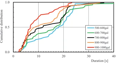
Figure 4 shows the cumulative distribution of duration of HCGMs of each acceleration range. The HGCMs incorporate various kinds of seismic sources and seismic-source characteristics, therefore the durations vary from under 5s to over 30s. It is found that the durations are long for low acceleration levels. The median duration in the acceleration range of 500 ~ 600 cm/s2 is about 18s and that of 900 ~ 1,000 cm/s2 is about 6.5s. This is because the number of ground motions from crustal earthquakes whose fault distances are small increase when the acceleration level is large. The median duration for 250 motions of HCGMs is 13.3s.
1 10 100
0.01 0.1 1 10
A cc . R es p . [c m /s /s ] Period [s] 900-1000gal 800-900gal 700-800gal 600-700gal 500-600gal
h = 0.01
0.0 0.1 0.2 0.3 0.4 0.5
0.01 0.1 1 10
C o m m o n lo g S .D . Period [s] 900-1000gal 800-900gal 700-800gal 600-700gal 500-600gal
h = 0.01
-1.0 -0.8 -0.6 -0.4 -0.2 0.0 0.2 0.4 0.6 0.8 1.0
0.01 0.1 1 10
C o rr el at io n c o ef . Period [s] h = 0.01
Reference period
0.04 ~ 0.1
0.2 ~ 1.0 2.0 ~ 10
(1) Median (2) log-standard deviation (3) Inter-period correlation
Figure 3. Statistics of response spectra (1% damping, on the free rock surface)
0.0 0.5 1.0
0 10 20 30 40
C u m u la ti v e d is tr ib u ti o n Duration [s] 500-600gal 600-700gal 700-800gal 800-900gal 900-1000gal
Figure 4. Cumulative distribution of duration
SIMULATED GROUND MOTIONS COMPARED WITH HAZARD-CONSISTENT GMs
differences between cases are the conditions of realizing the variation or the inter-period correlation of response spectra.
Table 3 describes the conditions for simulating ground-motions. The ground motions of case(n) were generated with no variation in response spectra. The ground motions of case(p) were generated to have the same variation of response spectra with case(r), however the coefficients of inter-period correlation are 1.0. The ground motions of case(c) were generated the way of incorporating the same variation and inter-period correlation of response spectra with case(r). The right column of Table 3 illustrates the inter-period correlation model for case(c). The inter-period correlation model for case(c) was set based on the results of HCGMs, which are ground motions of case(r), shown in Figure.3. The duration of simulated ground motions of case(n), case(p) and case(c) was set as 10s on the basis of the results of HCGMs. For the envelope, was Jennings type of function was applied.
Figure 5 shows the statistics of simulated ground motions. Figure 5(1) and (2) shows respectively the median and common log-standard deviation calculated from response spectra of simulated ground motions for all cases. It can be confirmed that found that the median response spectra in each case show good agreement with that of case(r). As for the variation of response spectra, the deviations of case(p) and case(c) indicate smaller values than those of case(r) in long period. The deviations of case(n) show larger values than the target deviation, 0.0.
Table 3: Conditions for simulating ground motions.
1 10 100
0.01 0.1 1 10
A cc . R es p . [c m /s /s ] Period [s] case(n) case(p) case(c) case(r)
h = 0.01
0.0 0.1 0.2 0.3 0.4 0.5
0.01 0.1 1 10
C o m m o n lo g S .D . Period [s] case(c) case(p) case(n) case(r)
h = 0.01
-1.0 -0.8 -0.6 -0.4 -0.2 0.0 0.2 0.4 0.6 0.8 1.0
0.01 0.1 1 10
C o rr el at io n c o ef . Period [s] case(c) Reference period
0.04 ~ 0.1
0.2 ~ 1.0 2.0 ~ 10 h = 0.01
Figure 5 Statistics of response spectra of simulated ground motions (1% damping, 700~800cm/s2).
SEISMIC RESPONSE ANALYSIS OF GENERAL RC STRUCTURE
Structural Model
Table 4 shows the soil condition at reference site and skeleton curve of structure for 1st floor. The soil of No.5 is the engineering bedrock and No.7 is the bedrock. In the response analysis, the surface soil of No.1 ~ No.4 was ignored and the structural basement was set on the soil layer, No.5.
Case
Response spectra Inter-period correlation model for case(c)
Median Deviation Inter-period correlation
case (r) Original HCGMs
case (n)
Median response spectra
of case(r)
No variation -
case (p) The same as case(r) Perfect correlation
case (c) The same as case(r) Modeled inter-period
correlation of case(r)
(1) Median (2) log-standard deviation (3) Inter-period correlation
-1.0 -0.8 -0.6 -0.4 -0.2 0.0 0.2 0.4 0.6 0.8 1.0
0.01 0.1 1 10
C o rr el at io n c o ef . Period [s] Reference period
0.04 ~ 0.1 0.2 ~ 1.0
Seismic response analyses were conducted for a simple structural model supposed general RC structure which has 4 stories. The structure is modelled as multi-mass shear system with the basement, which does neither swaying nor rocking. The mass and the height of structure are assumed the same values for each story. The stiffness ratio of each story and the initial stiffness of 1st story are decided so that each story drift caused by Ai distribution external force is the same value and the frequency of first vibration mode of the structure is 4.3Hz, which is the same value with that of PWR building. For the non-liner characteristics of shear spring, Takeda model was applied, which is tri-non-liner characteristics where the story drift angle at elastic limit R1 is 1/2,870 radian and the angle at yield point R2 is 1/478 radian. The
stiffness degrading ratio at elastic limit is 0.2 and that at the yield point is 0.005. The damping ratio of response spectra is targeted for 5 % or 1 %, for evaluating responses of equipment as well as of the structure.
Table 4: Soil characteristics at reference site and skeleton curve for structure.
Soil characteristics Structure characteristics of 1st floor
N o.
Soil layer width
(m)
Weight (kN/m2)
Modulus of rigidity (kN/m2)
Damping
(%) Notification
1 2.39 13.9 50.4 1.70 -
2 5.66 18.5 298 0.68 -
3 6.96 17.6 ~ 18.5 154 ~ 298 0.68 ~ 1.73 -
4 11.01 18.5 ~ 19.6 298 ~ 605 0.0 ~ 0.68
5 64.91 18.2 ~ 18.4 318 ~ 345 0.46 ~ 0.74 Engineering
bedrock
6 83.78 17.8 463 ~ 694 2.04
7 ! 19.3 2020 2.04 Bedrock
Maximum Structural Response and Inter-mass Correlation
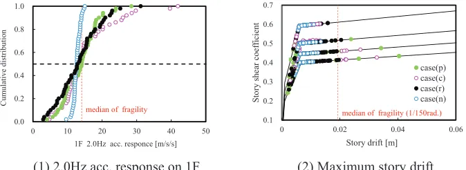
Figure 6 represents the results of maximum structural response by the ground motions in 700~800 cm/s2. Figure(1) shows the cumulative distributions of acceleration response on the 1st floor. Figure(2) shows the maximum story drift of structure. In these figures, the red dotted lines represent the median of fragility for equipment in Figure 7. In figure(1), almost the same distributions can be seen for case(r), case(p) and case(c), however the structural response variation of case(n) is smaller than other cases, because the variation of input ground motions is smaller than others. In figure(2), the story drifts of case(n) indicate the smallest variation and those of case(p) show the largest variation.
0.0 0.2 0.4 0.6 0.8 1.0
0 10 20 30 40 50
C
u
m
u
la
ti
v
e
d
is
tr
ib
u
ti
o
n
1F 2.0Hz acc. responce [m/s/s] median of fragility
0.1 0.2 0.3 0.4 0.5 0.6 0.7
0 0.02 0.04 0.06
S
to
ry
s
h
ea
r
co
ef
fi
ci
en
t
Story drift [m]
case(p) case(c) case(r) case(n)
median of fragility (1/150rad.)
Figure 6. Results of response analysis (700 ~ 800cm/s2).
K0
Story drift angle 0.005K0
0.2K0
Base shear coefficient CB
Rmax
0.4
0.2
R2 R1
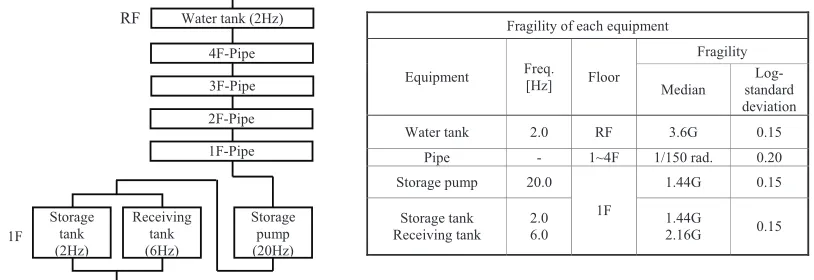
Equipment System and Fragility of equipment
The building function loss evaluation was conducted for simple plumbing system settled on the structure mentioned above. The equipment system tree, the median, deviation and natural frequency of equipment are shown in Figure 7. The plumbing system consists of storage tank, receiving tank, storage pump, pipes, and water tank. The water is pumped by storage pump from water tanks on 1st floor to the water tank on roof floor through pipes. The storage tank and receiving tank on the 1st floor are connected as parallel units, and these tanks, storage pump, pipes and water tank are connected as series units.
The fragility for equipment is assumed to represent the log-normal distribution. The damages of tanks and pumps are decided by the maximum floor acceleration response at their natural frequency, and those of pipes are by the maximum story drift angle.
Here, the median of fragility is assumed to be 3.6 times of design values for the equipment of seismic importance “B” class, which is defined in the guidelines of seismic design for building utility by BCJ (2005), because the acceleration level of targeted ground motions are so large for general equipment. The median of fragility for storage tank (2.0Hz) is set as the 2/3 times of median for receiving tank (6.0Hz) so that the damage probability of each tank becomes almost equal. The natural log-standard deviation of fragilities is set as 0.15 according to seismic PRA guidelines of AESJ (2007). As for the fragility for pipes, the median is 1/150 radian and the deviation is 0.20.
Figure 7. Equipment system tree and Fragility of equipment.
DAMAGE PROBABILITY OF SYSTEM
From the maximum structural response by the seismic analysis for each ground motion, the damage probability of equipment is calculated based on the fragility in Figure 7, and the damage probability of the system is evaluated based on the system tree in Figure 7. The damage probabilities of the system are averages over 50 motions in each acceleration range. The right 4 columns in Table 5 show the damage probabilities of the system for each acceleration range and for each case. In the bottom row of the table, the annual damage frequencies of the system by 500 ~ 1,000 cm/s2 ground motions are listed. These are evaluated with the damage probability of the system for each acceleration range and its annual frequency which are listed in the 2nd column of the table.
The annual system damage frequencies of case(r) and case(c) are about 100x10¬6, almost the same values. Therefore, it can be said that almost the same damage frequency is obtained when the variations and inter-period correlations of response spectra are realized for simulating ground motions. The annual system damage frequencies of case(n) is about 60x10¬6, which is smaller than that of case(r). The results clearly show that the response spectra variations of input ground motions have severe influence on resulted damage probabilities. Damage probabilities of case(n) by 50 motions of 700 ~ 800 cm/s2 range show almost the same values with those of other cases, while larger probabilities are obtained for high
Fragility of each equipment
Equipment Freq.
[Hz] Floor
Fragility
Median
Log-standard deviation
Water tank 2.0 RF 3.6G 0.15
Pipe - 1~4F 1/150 rad. 0.20
Storage pump 20.0
1F
1.44G 0.15
Storage tank Receiving tank
2.0 6.0
1.44G
2.16G 0.15
RF
1F
Water tank (2Hz)
4F-Pipe
3F-Pipe
2F-Pipe
1F-Pipe
Storage pump (20Hz) Storage
tank (2Hz)
acceleration level and lower probabilities for low level. Because of small response spectra variation of case(n), the damage probability might be sensitive for the acceleration level. After all, the annual damage probability of case(n) is evaluated smaller than others, because damage possibilities are low for low acceleration level whose annual frequencies are large.
On the other hand, annual damage probability of case(p) is evaluated as 110x10¬6, the slightly larger values than those of case(r) and case(c). Therefore, it can be said that the effect of setting the correlation coefficient be 1.0 was observed. In this system, the damage probabilities depend on the damage probabilities of water tank on roof floor for low acceleration level, and weight of damage probabilities of tanks on 1st floor increase for higher acceleration levels. The damage probability of two tanks on 1st floor of case(p) is larger than other cases, because response correlation of two tanks in case(p) is higher than in other cases. However, the influence of the difference of response correlation on the system damage probabilities is not large.
As a result, the damage probabilities of system are more influenced by the variation than by the inter-period correlation of response spectra in this study.
Table 5 : Annual probability of hazard consistent ground motions.
Fragility of equipment system
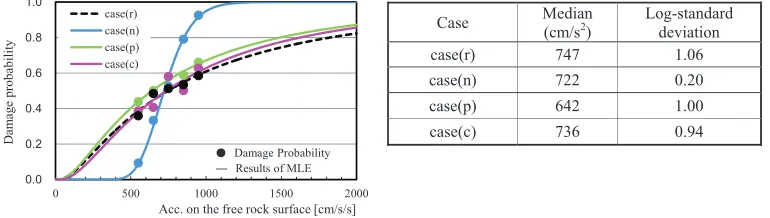
The fragility curves of equipment system are calculated with maximum likelihood evaluation (MLE) method, where the damage probability listed in Table 5 and the median of each acceleration range on the free rock surface are used as the index of the input.
Figure 8 shows the results of fragility curves, the median and deviation of fragility curves for each case. The fragilities of case(r) and case(c) are almost the same distribution, and that of case(n) indicate much smaller variation, therefore it indicate smaller damage probability in low acceleration level. The fragility of case(p) indicates a little larger value than those of case(r) and case(c).
0.0 0.2 0.4 0.6 0.8 1.0
0 500 1000 1500 2000
D
am
ag
e
p
ro
b
ab
il
it
y
Acc. on the free rock surface [cm/s/s] case(r)
case(n) case(p) case(c)
䖃 Damage Probability
" Results of MLE
Figure 8. Fragility of equipment system calculated from maximum likelihood evaluation method.
DAMAGE PROBABILITY OF NUCLEAR POWER PLANT SYSTEM
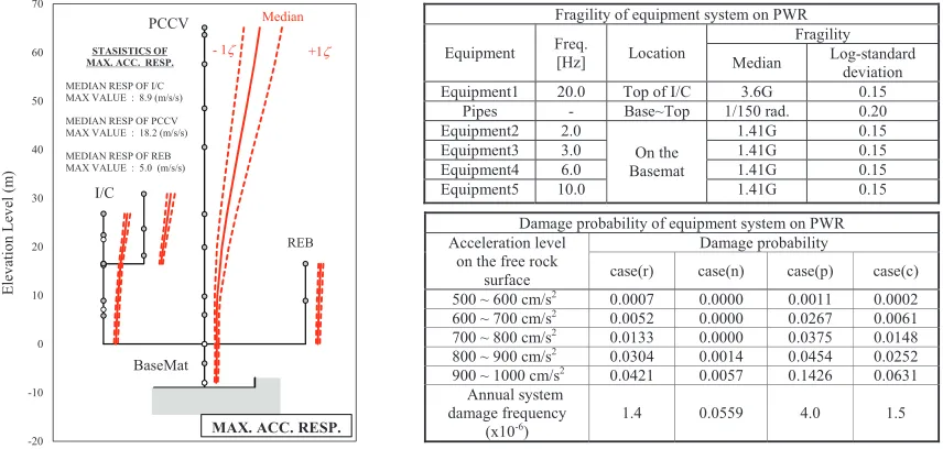
In this section, the response analysis and system damage probabilities evaluation of PWR building are conducted for ground motions of case(r)~(c). Figure 9 shows the examples of maximum
Acceleration level on the free rock surface
Annual frequency of ground motions (x10-6)
Damage probability
case (r) case(n) case(p) case(c)
500 ~ 600 cm/s2 131.4 0.359 0.093 0.438 0.387
600 ~ 700 cm/s2 54.1 0.485 0.333 0.501 0.407
700 ~ 800 cm/s2 24.8 0.512 0.527 0.579 0.581
800 ~ 900 cm/s2 12.4 0.534 0.790 0.589 0.502
900 ~ 1000 cm/s2 6.6 0.585 0.925 0.660 0.626
Annual system damage frequency (x10-6) 97 59 111 98
Case Median
(cm/s2)
Log-standard deviation
case(r) 747 1.06
case(n) 722 0.20
case(p) 642 1.00
acceleration response results by HCGMs (case(r), Igarashi et al. (2015) ) in the acceleration range in 700 ~ 800 cm/s2. The maximum responses by 250 motions of case(r) ~ case(c) were almost within elastic range. In the damage probability evaluation, the simple system is settled on the internal concrete (I/C) of PWR building. The system consists with 4 equipment on the basemat which are different from natural frequency, pipes and equipment on the top floor of I/C. The equipment on the basemat are assumed as parallel system, and the parallel unit, pipes and equipment on the top floor are connected as series units. The fragilities of equipment are decided as the values in Figure 9.
The results of damage probabilities and annual frequency of system are shown in Figure 9. The damage probabilities of case(r) and case(c) are almost the same values, and the same tendencies with general RC structure mentioned above are found to the PBR building.
Figure 9. Maximum acc. response of PWR building (700 ~ 800 cm/s2) and system damage prob.
CONCLUTION
In order to confirm the effectiveness of applying the hazard-consistent ground motions which incorporate the difference of seismic-source characteristics, the building function loss evaluation was conducted for equipment system settled on a general RC structure and PWR building. The hazard-consistent ground motions which are used for advanced PRA incorporate both of epistemic and aleatory uncertainties of seismic source characteristics. The ground motions which have been used for usual PRA scheme rarely incorporate detailed seismic-source characteristics. For example, they are generated to fit to specific response spectra, where the variation and/or inter-period correlation are not involved. In this context, three cases of ground motions set which were generated considering variation and inter-period correlation, case(n) ~ case(c), were examined by comparing their impact on the damage probabilities of the system with each other.
1) Almost the same system damage probabilities with case(r) were obtained for case(c), where ground motions of case(r) are hazard-consistent ground motions as they are, and in case(c), ground motions incorporate the same variation and inter-period correlation of response spectra, while their durations are constant.
2) Smaller damage probabilities than other cases are obtained for case(n) whose ground motions are generated without considering the variation of response spectra. The reasons are that the damage probabilities are low for low acceleration level whose annual frequencies are large.
Fragility of equipment system on PWR
Equipment Freq.
[Hz] Location
Fragility
Median Log-standard
deviation
Equipment1 20.0 Top of I/C 3.6G 0.15
Pipes - Base~Top 1/150 rad. 0.20
Equipment2 2.0
On the Basemat
1.41G 0.15
Equipment3 3.0 1.41G 0.15
Equipment4 6.0 1.41G 0.15
Equipment5 10.0 1.41G 0.15
Damage probability of equipment system on PWR Acceleration level
on the free rock surface
Damage probability
case(r) case(n) case(p) case(c)
500 ~ 600 cm/s2
0.0007 0.0000 0.0011 0.0002
600 ~ 700 cm/s2
0.0052 0.0000 0.0267 0.0061
700 ~ 800 cm/s2
0.0133 0.0000 0.0375 0.0148
800 ~ 900 cm/s2
0.0304 0.0014 0.0454 0.0252
900 ~ 1000 cm/s2
0.0421 0.0057 0.1426 0.0631
Annual system damage frequency
(x10-6
)
1.4 0.0559 4.0 1.5
-20 -10 0 10 20 30 40 50 60 70
!15 !10 !5 0 5 10 15
E
le
v
at
io
n
L
ev
el
(
m
)
PCCV
REB I/C
BaseMat
Median
+1#
- 1#
MAX. ACC. RESP.
STASISTICS OF MAX. ACC. RESP.
MEDIAN RESP OF I/C MAX VALUE : 8.9 (m/s/s)
MEDIAN RESP OF PCCV MAX VALUE : 18.2 (m/s/s)
3) It is found for the system examined in this paper that the variations of response spectra affect strongly on the damage frequencies of equipment system. On the other hand, the inter-period correlation of response spectra does not affect so strongly on them.
ACKNOWLEDGEMENT
The time history data of hazard-consistent ground motions used in this study were provided by Japan Atomic Energy Agency. We express gratitude here.
REFERENCES
D.L.Wells and K.J.Coppersmith (1994). “New Empirical Relationship among Magnitude, Rupture Length, Rupture Width, Rupture Area, and Surface Displacement”, Bulletin of the Seismological Society of America, 84(4), 974-1002.
Igarashi, S., et al. (2015). “Structural response by Ground Motions from Sources with Stochastic Characteristics”, ICONE-23.
Irikura, K. and Miyake, H. (2001). “Prediction of Strong Ground Motions for Scenario Earthquakes (in Japanese)”, Journal of Geography, 110(6), 849-875.
Ishii, T. and Sato, T. (2000), “Relations between the Main Rupture Areas and their Moments of Heterogeneous Fault Models for Strong-motion Estimation (in Japanese)”, The Seismological Society of Japan, B09.
Matsuda, T. (1975). “Magnitude and Recurrence Interval of Earthquakes from a Fault”, Jishin, 2(28), 269-283.
Nishida, A., et al. (2013). “Characteristics of Simulated Ground Motions Consistent with Seismic Hazard”, SMiRT-23.
Noda, S., et al. (2002). OECD-NEA Workshop on the Relations between Seismological Data and Seismic Engineering Analysis.
Nuclear Standards Committee of JEA (2008). “Technical Code for Seismic Design of Nuclear Power Plant”.
Sato, R. (1989). “Handbook for Parameters of seismic faults in Japan (in Japanese)”.
Sakamoto, S., et al. (2014). “Dynamic Analysis of Structures with Hazard Consistent Ground Motions (Part 1) (in Japanese)”, AIJ, 3-4.
Shimazaki, K. (1986). “Small and large earthquakes, The effect of the thickness of seismologenic layer and the free surface”, Earthquake Source Mechanics, AGU Geophysical Monograph, 37, 269-283. Somervile et al. (1999). “Characteristics Crustal Earthquakes Slip Models for the Prediction of Strong
Ground Motion”, Seismological Research Letters, 70(1). Standards Committee of AESJ (2007), “AESJ-SC-P006:2007”
Takada, T., et al. (2014). “Comparison with Ground Motions Generated by Different Methods Considering Source Uncertainties (in Japanese)”, AIJ, 1-2.
Takemura et al. (1990). “Scaling Relation for Source Parameters and Magnitude of Earthquakes in the Izu Peninsula Region, Japan, Tohoku”, Geophys.Journal, 32(3), 4, 77-89
Takemura, M. (1998). “Scaling Law for Japanese Intraplate Earthquakes in Special Relations to the Surface Faults and the Damages.(in Japanese)”, Jishin, 2(51), 211-228.
The Building Center of Japan (2005). “Guideline of seismic design and application of building utility (in Japanese)”.