Maximum Likelihood Analysis of Rare Binary Traits Under Different Modes of Inheritance

(1)

Copyright 8 1996 by the Genetics Society of America

Maximum Likelihood

Analysis

of Rare

Binary

Traits

Under Different Modes of Inheritance

**G. Thder,'t L. DempfleI'**

and

I. Hoeschelety'

*Znstitut f u r Timissenschafen, Technische Universitat Munchen-Weihenstephan, Germany and +Department of Dairy Science, Virginia Polytechnic Institute and State University, Blacksburg, Virginia 24061

Manuscript received June 19, 1995

Accepted for publication April 24, 1996

ABSTRACT

Maximum likelihood methodology was applied to determine the mode of inheritance of rare binary traits with data structures typical for swine populations. The genetic models considered included a monogenic, a digenic, a polygenic, and three mixed polygenic and major gene models. The main emphasis was on the detection of major genes acting on a polygenic background. Deterministic algorithms were employed to integrate and maximize likelihoods. A simulation study was conducted to evaluate model selection and parameter estimation. Three designs were simulated that differed in the number of sires/number of dams within sires (10/10, 30/30, 100/30). Major gene effects of at least one SD of the liability were detected with satisfactory power under the mixed model of inheritance, except for the smallest design. Parameter estimates were empirically unbiased with acceptable standard errors, except for the smallest design, and allowed to distinguish clearly between the genetic models. Distributions of the likelihood ratio statistic were evaluated empirically, because asymptotic theory did not hold. For each simulation model, the Average Information Criterion was computed for all models

of analysis. The model with the smallest value was chosen as the best model and was equal to the true model in almost every case studied.

S

TATISTICAL analyses of mixed major gene and polygenic inheritance models (e.g., KNOTT et al. 1991a,b; JANSS et al. 1995) or of linkage between Quanti-

tative trait loci (QTL) and genetic markers (e.g., Guo and THOMPSON 1992; KNOTT and HALEY 1992) have been applied to continuous measurements rather than to binary or categorical data. For the latter, a polygenic or mixed model of inheritance may be postulated based on the threshold concept (ELSTON and STEWART 1971; GIANOLA and FOULLEY 1983; FALCONER 1986).

Several statistical methods can be applied to determine the most likely mode of inheritance and to obtain parameter estimates. While there are a number of simple statistical tests for the presence of a major gene (HILL and KNOTT 1990), there are two methods that are most powerful and enable most accurate estimation of genetic and nongenetic parameters, unless the data severely violate the assumptions imposed by the methods. These methods are complex segregation analysis

by maximum likelihood (ML) (ELSTON and STEWART

1971; MORTON and MCLEAN 1974) and Bayesian complex segregation analysis (HOESCHELE 1988; JANSS et al. 1995).

In ML, the likelihood function of the observed data is

Curresponding authm: I. Hoeschele, Department of Animal and

Range Sciences, Montana State University, Bozeman, MT 59717.

E-mail: [email protected]

Gambia.

Present address: International Trypanotolerance Centre, Banjul,

On leave from Virginia Polytechnic Institute and State University.

Genetics 143: 1819-1829 (August, 1996)

maximized with respect to all parameters in the model postulated, and hypothesis testing is based on the likelihood ratio statistic. In this paper, we present, under the standard mixed model of inheritance, the classical ML methodology for complex segregation analysis of binary disease traits with data structures representative of swine populations (dams nested within sires and hav- ing multiple offspring) and with parents assumed free of the disease. In another contribution (THALLER et al. 1996), this method was employed to analyze actual data on 32,621 litters and eight binary disease traits in swine. These traits were chosen because their mode of inheritance had not been determined previously from a sufficient range of modes including the mixed. Here, we present results from a simulation study, which was conducted to validate the methodology used for the analysis of actual data. The ML analysis was implemented deter- ministically using numerical integration and derivative- free maximization. Ability to select the correct mode of inheritance and accuracy of parameter estimation were evaluated for three designs increasing in size.

METHODOLOGY

In this section, we first describe the genetic models considered in this study. We then present the classical likelihood for binary disease data under the mixed model of inheritance, followed by deterministic algorithms to implement the ML analysis.

(2)

1820 G. Thaller, L. Dempfle and I. Hoeschele

genetic models can be postulated that differ in the number of loci, the number of alleles per locus, and the relationship between phenotypes and genotypes. Limi- tations in computing and statistical power prohibit comparisons among a large number of models. Therefore, several models were selected that cover a wide range of possible modes of inheritance. The oligogenic models were represented by a one-locus and a two-loci model, each locus being biallelic. In the monogenic model, the defect-causing gene was assumed to be recessive.

Digenic models allow various assignments of affectedness to the genotypes (HARTL and MARUYAMA, 1968). Out of these, the double homozygous recessive model was considered to be most appropriate for a rare disease, with the two loci being unlinked. This digenic model and a model where all individuals being recessive homozygous at at least one locus are affected were used in an analysis of actual data (THALLER et al. 1996). Across all eight traits considered, the double homozygous recessive model provided a much better fit to the data than the single homozygous recessive model and was therefore chosen to represent the digenic models in this investigation.

The purely polygenic model assumed a normally dis- tributed underlying liability with a single threshold and with individuals affected when their liability exceeded the threshold value (FALCONER, 1986). The monogenic and polygenic models were special cases of the classical mixed model of inheritance, which includes the fixed effect of the genotype at a biallelic major locus and a polygenic effect. The mixed model used in this investigation was, in matrix notation,

y = X @ + W T a + Z u + e

Var(u) = AD:, Var(e) = Za:, af = 1, (1)

where

y

was vector of unobserved liabilities of offspring,

p

was vector of fixed effects, X was a design-covariable matrix relating liabilities to fixed effects and possibly containing columns with covariates, (Y was vector of ma-

jor locus parameters a and d, a was half of the homozygote difference, d was dominance deviation, W was an incidence matrix relating liabilities to major genotypes,

T

was matrix relating the three major genotypes to the parameters a and d, u was vector of additive polygenic values, Z was an incidence matrix relating liabilities to the polygenic values, and A was the additive genetic or numerator relationship matrix (HENDERSON 1976).

Classical ML analysis: The likelihood for the classical ML analysis was derived for a hierarchical halfsibfull- sib structure typical for swine populations with one litter per dam. The observed data were the discrete phenotypes with Yqk = 0 for unaffected offspring

K

of dam

j

within sire i and

Elk

= 1 for an affected offspring. After some algebra, the likelihood of the numbers of unaffected ( N , -

K j )

and affected ( Y y . ) offspring in all

litters, given the sires ( i = 1 ,

. .

.

,

S) and dams (i = 1,

. . .

,

D,)

are unaffected and unrelated, could be written as

TABLE 1

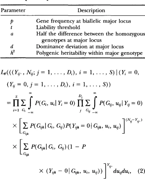
Description of parameters in the models considered

Parameter Description

P

Gene frequency at biallelic major locus t Liability threshold

a Half the difference between the homozygous

d h2

Dominance deviation at major locus

Polygenic heritability within major genotype genotypes at major locus

where S was number of sires, Dj number of dams within sire i, 8 was the parameter vector with 8' =

[p,

a,

d, t, h 2 ] , the parameters in 0 were as described in Table 1, G was major genotype,

ui

was the additive polygenic value of sire i, and uli was the additive polygenic value of dam j nested within sire i. Furthermore, in Equation

2

P( Gqkl Gj, G,) represents the standard Mendelian transmission probability at a single locus. The condi- tional joint probability density of sire major genotype and polygenic value in

(2)

was

where

P(K = 0 ) =

C

P ( G i ) @ ( t - g a ) .

Gi

(3)

Inheritance of Rare Binary Traits 1821

-m

m

-m

where +(q p x , a:) is the density of N ( p , ,

ai).

The last equality was obtained after some algebra and using a result of Curnow (1984) for integrating the product of the standard normal density (evaluated at x) and Q ( a

+

b x ) for some known constants a and 6.

For hypothesis testing, twice the difference in the natural logarithms of the likelihoods of a full and a restricted model was computed,

T = 2 ln[ML(Rl)]-2 ln[ML(Ro)], (5)

where ML(Rl ) is the likelihood maximized under the full model, and ML(Ro) is the likelihood maximized under the restricted model. T was also computed for nonnested models. Under certain conditions, T has an asymptotic chi-squared distribution. Unfortunately, the asymptotic theory does not hold in the following three cases: (1) Neither of the two models compared is nested within the other, (2) there are constraints on a parameter being fixed at the boundary of its space under the null hypothesis (TITTERINGTON 1985), and ( 3 ) the number of degrees of freedom is unclear in certain situations. Here, case (1) applies, e.g., to a comparison between the polygenic and monogenic models, case (2) to the mono- and digenic models, and case ( 3 ) to the polygenic and mixed models, where the polygenic model contains at least two parameters less than the mixed model, but restricting only one parameter, e.g., setting gene frequency

p

= 0 , will reduce the mixed to the polygenic model. Cases

(2)

and ( 3 ) are well known in the general context of finite mixture distributions

(TITTERINGTON et al. 1985). In all three cases, the distribution of the test statistic can be found empirically by simulation or data permutation (CHURCHILL and DOERCE 1994) in simulation studies and real data analyses, respectively, provided that these are computationally feasible. Furthermore, any models, including nonnested models, can be compared using Akaike's Average Information Criterion (AIC) (AKAIKE 1973), which, however, relies on asymptotic normality of the ML estimators. When conditions for this property are not satisfied, the AIC can still be used as an approximation (Wm-4 and KASHIWAGI, 1990). Adding to T the term 2(ro - q), where rj is the number of parameters fitted under model i ( i = 0 , l ) , yields the difference

between the AIC for model 0 and the AIC for model 1 . Small values of AIC, which equals twice the number of (independently adjusted) parameters minus twice the log likelihood, are desirable, hence the model with the smallest AIC value should be chosen.

Deterministic algorithms for ML: Computing the likelihood in (2) requires performing the integrations over the sire and dam effects, respectively. In general, integrals of the form

s s

n

g(z) dz = eP2flz)dz = W&G)

i- 1

-m "m

can be approximated by a weighted summation as shown by NAYLOR and SMITH (1982). Effectively a continuous density function is replaced by a discrete histo- gram, and suitable weights w, and abscissae G have to be supplied. Increasing the number of points in the summation improves the approximation and efficient weights as well as abscissae can be obtained from the Hermite polynomial as the integrand is in the form exp ( -

2 )

( KNOTI et al. 199 l a ) . Tables of abscissae and corresponding weights for various numbers of points are available (e.g., ~ R A M O W I T Z and STECUN 1970).

After substituting ( 3 ) and (4) in (2) the integrands can be rewritten as a product of the normal density flui) with a regular function h ( u i ) for the sire effect and as a product off(uq) with a regular function h(u,) for the dam effect, respectively. Because of the complex- ity of the resulting formula, the numerical integration is demonstrated only for the sire's transmitting ability

ui but applies analogously to the integration over uq. The integrand is

and allowing for ui to have a nonzero mean and a variance different from 1 leads to the explicit expression

Replacing the argument in the exponent by x = (u,

- and transforming ui and dui appropriately

results in

+ m

(4)

1822 G. Thaller, L. Dempfle and I. Hoeschele

TABLE 2

List of models considered and their parameters

Model Parameters

One-locus, monogenic

P

Two-loci, digenic

(double recessive homozygotes affected)

p, q

Polygenic h2, t

Mixed ( d = “a or d = 0) h2, a, d,

p,

t

Initial analyses showed that 10 points yielded sufficient precision. This finding is in agreement with results obtained by KNOTT et al. (1991a).

For maximization of likelihoods, the Powell algo- rithm (PRESS et al. 1986), a derivative-free approach only requiring multiple likelihood evaluations, was chosen. To ensure that the maximum was located within the parameter space, a very small likelihood was as- signed to invalid parameter combinations. The chance of finding a local rather than a global maximum was reduced by using several sets of starting values. Differ- ences in the maximized likelihoods corresponding to different sets of starting values were mostly obtained under the mixed model with the smallest major gene effect (see SIMULATED DATA below), where this occurred in -15% of all analyses. The largest likelihood with corresponding parameter estimates was retained in such cases.

SIMULATED DATA

Data sets were simulated under the six genetic models described in Table

2.

Three data structures were chosen with different numbers of sires and dams within sires. Design 10/10 consisted of 10 sires and 10 dams per sire, design 30/30 of 30 sires and 30 dams per sire, and design 100/30 of 100 sires with 30 dams per sire. Litter size was fixed at 10 offspring in each design. These designs were chosen because the number of 30 dams per sire was in good agreement with actual data analyzed, and because design 100/30 was the largest possible design allowing for sufficient replication from a computational standpoint.

Out of a generated base population, only unaffected parents were selected and mated randomly. The frequency of the favorable dominant allele was 0.8 in the monogenic and

0.7

at both loci in the digenic model. Data sets with polygenic inheritance were simulated using a heritability of the underlying liability of 0.5. For the data sets generated under the mixed model, allele frequency was 0.8, polygenic heritability was 0.5, and the gene effect at the major locus equaled 0.5, 1, or 2 times the standard deviation of liability (a,) within major genotype. These three mixed models will later be referred to as the small, intermediate, and large mixed model, respectively. Incidence of disease for the discrete loci models was determined by allele frequencies, and in the liability models, the threshold was set to a value resulting

TABLE 3

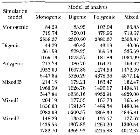
Averages of ML values for different true models and models of analysis

Model of analysis Simulation

model Monogenic Digenic Polygenic Mixed

Monogenic 84.29 83.95 103.04 83.85

719.74 720.01 878.90 719.67

2358.37 2360.60 2885.37 2358.37 Digenic 44.29 40.42 43.18 40.06

361.59 329.23 359.54 336.69

1169.13 1073.37 1181.83 1084.99 Polygenic 217.73 180.70 164.21 163.62

1953.00 1607.88 1474.54 1472.39

6447.84 5320.29 4878.36 4877.14

Mixed05 214.13 179.21 163.47 162.47

1960.59 1626.76 1496.17 1494.31 6447.84 5358.16 4932.91 4929.00

Mixed1 204.19 177.53 167.73 165.54

1856.08 1591.97 1489.34 1480.84 6082.08 5200.37 4868.30 4846.81

Mixed2 148.29 135.56 135.57 127.67

1435.53 1307.83 1260.20 1200.54 4782.70 4365.93 4216.88 4012.37

First figure in each cell is for design 10/10, second for 30/ 30, third for 100/30.

in 5% affected animals in the base population. Design 10/10 was replicated 100 times, while the number of replicates was reduced to 50 for designs 30/30 and 100,’ 30 due to computational constraints.

Additional data sets (A) were generated for design 30/30 and a mixed model with major gene effect 2a,, polygenic heritability of 0.5, allele frequency of 0.9 and incidence of 0.05. These data sets were used to investi- gate the so-called Extreme Category Problem (MISZTAL and GIANOLA 1989).

RESULTS AND DISCUSSION

Model selection: All simulated data sets, except for the additional data sets (A), were analyzed with all genetic models using the classical ML methodology. Aver- ages of the (-2 In ML) values (from here on referred to as ML values) are given in Table 3 for the three different designs. Any two models may be compared by computing T in ( 5 ) , however one can generally not assume that T has a known asymptotic chi-squared distribution. Within each column, corresponding to a particular model of analysis, the AIC value can be obtained by adding 2 to all values in the column for the monogenic model, 4 to all values in the columns for the digenic and polygenic models, and 8 to all values in the column for the mixed model. It is not clear whether 6 should be added to the column for the mixed model rather than 8, however, most of the results presented below were not affected by this number.

For data sets generated under the monogenic model,

(5)

Inheritance of Rare Binary Traits

TABLE 4

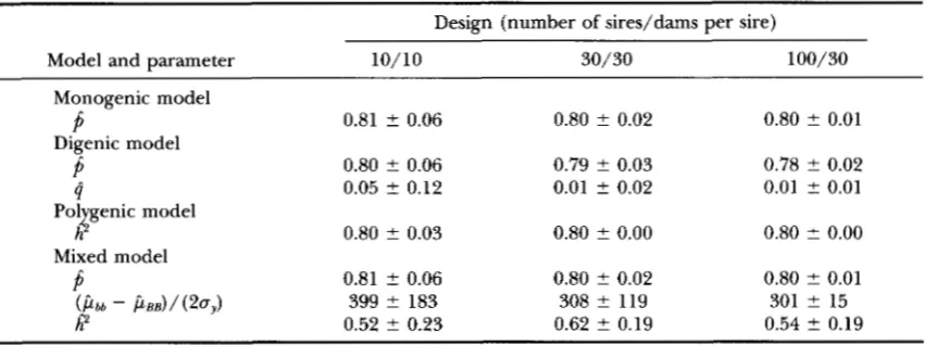
Average parameter estimates and empirical standard errors; true state: one-locus model

Design (number of sires/dams per sire)

Model and parameter 10/10 30/30 100/30

Monogenic model

Digenic model

P

0.81 t 0.06 0.80 ? 0.02 0.80 ? 0.01

P

0.80 2 0.06 0.79 ? 0.03 0.78 ? 0.02

4

0.05 2 0.12 0.01 ? 0.02 0.01 2 0.01

Pol genic model

Mixed model

h

.t:

0.80 ? 0.03 0.80 ? 0.00 0.80 2 0.00

P

0.81 t 0.06 0.80 ? 0.02 0.80 ? 0.01

P

0.52 ? 0.23 0.62 0.19 0.54 t 0.19

( P b b - P B B ) / ( 2 0 y ) 399 ? 183 308 ? 119 301 ? 15

1823

values that were either the lowest or very near the lowest values. The ML values obtained from analysis under the polygenic model were highest, indicating that it is most unlikely in all three designs. The ML values of the digenic model were slightly lower than the ML values for the monogenic model in design 10/10, but somewhat higher in designs 30/30 and 100/30. This result con- firms that one cannot expect a difference of 1 due to constraints on the gene frequency parameters. All replicates in designs 30/30 and 100/30 had their maximum at the boundary of the parameter space with one of the allele frequencies being zero, hence the ML values were equal to those of the monogenic model. In a few replicates, the maximum was not attained due to difficulties in searching at the boundary, which resulted in compar- atively high ML values and a biased average. For the mixed model, the ML values also approached those of the monogenic model for the larger data sets. The parameter solutions achieving these ML values were characterized by extremely large major gene effects (a)

relative to the within genotype standard deviation. Con- sequently, the major genotype perfectly determined the outcome (affected or unaffected) without modifjmg influence of the within genotype variation. In terms of the AIC criterion, the monogenic model had the lowest value across all models of analysis and for each design, resulting in the choice of the correct model.

When the digenic model was the true state of nature, the same model of analysis yielded the lowest ML values except for design 10/10, where the mixed model attained the smallest value. The average differences to the monogenic model increased with the amount of data. The polygenic model fitted the data poorly, while the mixed model provided somewhat better ML values. In general, the differences between the ML values of the polygenic or mixed and the digenic model were large, in particular, for design 100/30 and the polygenic model. Based on the AIC criterion, again the true digenic model had the smallest value for all designs and was hence correctly identified.

Analyzing the data sets generated under the polygenic

model confirmed the expected high power in distinguishing between poly- and oligogenic inheritance. The ML values of the monogenic and digenic models were both very high indicating a bad fit. The differences of the ML values between the polygenic and the mixed models were in the range of 1 to 2. In terms of the AIC criterion, again the correct (polygenic) model was chosen for all three designs.

The data sets simulated under the mixed model were fitted poorly by both discrete loci models as expected. The ML values for the polygenic model were only slightly higher than those for the mixed model, when the major gene effect was only one-half of the standard deviation of liability. The differences between the ML values of the mixed and the polygenic model became larger with increasing amount of data. Using the AIC criterion, the mixed model was correctly identified for all designs when the major gene effect equaled

2

oy,

and for designs 30/30 and 100/30 when the major gene effect was 1 oy For the small major gene effect (one- half of a standard deviation), the polygenic model had the smallest AIC values in all three designs. This also occurred for the intermediate major gene effect and the small design 10/10.

Overall, in the vast majority of the cases studied, the true mode of inheritance was identified correctly based on the AIC criterion.

Parameter estimates: Average parameter estimates and their empirical standard errors obtained from analyses of data sets simulated under the monogenic model

(6)

1824 G . Thaller, L. Dempfle and I. Hoeschele

TABLE 5

Average parameter estimates and empirical standard errors; true state: digenic model

Model and parameter 10/10 30/30 100,’ 30

Monogenic model

Digenic model

P

0.89 5 0.04 0.90 5 0.01 0.90 ? 0.01

P

0.77 ? 0.09 0.75 ? 0.06 0.76 ? 0.05

B

0.50 ? 0.25 0.60 ? 0.15 0.60 t 0.12

Pol genic model

Mixed model

h

4

0.70 t 0.03 0.80 t 0.00 0.80 ? 0.00

P

0.92 ? 0.06 0.90 2 0.05 0.86 2 0.03

w

0.49 t 0.32 0.62 ? 0.29 0.62 ? 0.23

( P b b - bBB)/(20y) 159 ? 239 19.4 ? 70.1 1.85 2 0.73

under the monogenic model, and heritability was estimated with large standard error even for the largest design, which was a result of the lack of influence of the withingenotype variation on the likelihood due to the huge major gene effect.

Average parameter estimates and their empirical standard errors obtained from analyses of data sets simulated under the digenic model are presented in Table 5. Under the monogenic model, the data were best fitted with an allele frequency of 0.9, which results in a frequency of homozygous recessives (0.01) near that under the true digenic model (0.0081). Under the digenic model, allele frequency

( p )

at the first locus was fitted first and was overestimated, while frequency at the second locus ( q ) , fitted subsequently, was underestimated with larger standard error. Across both loci, the average frequency was underestimated, but this downward bias decreased with increasing size of the design. For the polygenic model, heritability was again estimated at or near the upper boundary. Under the mixed model, allele frequency estimates were similar to those obtained with the monogenic model. Estimates of the homozygote difference at the major locus were still very large but decreased with increasing design size. This

decrease was accompanied by a slight reduction in allele frequency, increasing overestimation of polygenic heritability and decreasing standard error of h2.

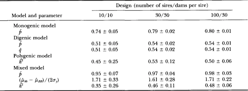
Average parameter estimates and their empirical standard errors obtained from analyses of data sets simulated under the polygenic model are presented in Table 6. The monogenic model fitted best with an allele frequency near 0.8, while the digenic model attained its best fit with allele frequencies at both loci near 0.5. Heritability was estimated unbiasedly and with substan- tial increases in accuracy for the larger designs, when the model of analysis was the same as the simulation model. With the mixed model, homozygote difference at the major locus was large but allele frequency was estimated near 1, resulting in a small variance at this locus. Heritability was underestimated, but to a decreasing extent with increasing design size and allele frequency estimates approaching 1 more closely.

Average parameter estimates and their empirical standard errors obtained from analyses of data sets simulated under the small mixed model are presented in Table

7.

Under the monogenic model, the average estimate of allele frequency was near the true frequency of the major gene but also the same as the estimate

TABLE 6

Average parameter estimates and empirical standard errors; true state: polygenic model

Design (number of sires/dams per sire) -

Monogenic model

Digenic model

P

0.74

t 0.05 0.79 ? 0.02

P

0.51 5 0.05 0.54 ? 0.02

(i 0.51 ? 0.05

0.80 2 0.01

0.54 ? 0.01 0.54 t 0.02 0.54 t 0.01

h

4

0.45 ? 0.25 0.53 2 0.12 0.50 2 0.06

0.98 2 0.03 Pol genic model

Mixed model

P

0.95 ? 0.07 0.97 2 0.04

I? 0.35 t 0.26 0.46 ? 0.11 0.48 ? 0.06

(7)

Inheritance of Rare Binary Traits

TABLE 7

Average parameter estimates and empirical standard errors; true state. mixed model; major gene effect of 0.5 av

Monogenic model

Digenic model

P

0.74 ? 0.05 0.79 ? 0.02 0.80 2 0.01

P

0.51 ? 0.05 0.54 ? 0.03 0.54 ? 0.01

4

0.51 2 0.05 0.54 2 0.03 0.54 ? 0.01

ff

0.51 ? 0.23 0.56 ? 0.13 0.51 t 0.06

P

0.66 ? 0.27 0.71 2 0.31 0.65 t 0.24

ff

0.30 ? 0.28 0.47 ? 0.15 0.49 ? 0.08

Polygenic model

Mixed model

( P b b - D E B ) / (20,) 1.05 ? 0.79 1.04 ? 0.68 0.72 ? 0.52

1825

obtained when the true state of nature was the polygenic model. Similarly, the allele frequencies in the digenic model were again estimated near 0.5. Under the mixed model, allele frequency at the major locus was clearly underestimated, which compensated, at least partially, for an overestimation of the homozygote difference. The latter decreased substantially, while the downward bias of polygenic heritability vanished, with increasing size of the design. Genetic variance at the major locus, with d = -a, equals V, = 4p2( 1 -

p’).’.

While the true value for V, was 0.2304, the estimated value decreased from 1.084 for the smallest design to 0.506 for the largest design, still overestimating the true value by over 100%.

Average parameter estimates and their empirical standard errors obtained from analyses of data sets simulated under the intermediate mixed model are presented in Table 8. Estimates of allele frequencies computed with the monogenic and digenic models of analysis were very similar to those obtained when the polygenic and the small mixed model were the true states of nature. Under the polygenic model, heritability was estimated

not far from its upper boundary with the larger major gene present. For the mixed model, allele frequency at the major locus was much more accurately estimated with the intermediate major locus segregating than with the small locus (Table 7). Homozygote difference was overestimated for the small design, while the upward bias vanished with increasing size of design. Major locus variance V, was still overestimated, with the true value being 0.922 and its estimates for the small and large designs equal to 1.779 and 0.992, respectively. As the upward bias of the major gene variance decreased with increasing design size, the downward bias of the polygenic heritability estimates was reduced.

Average parameter estimates and their empirical standard errors obtained from analyses of data sets simulated under the large mixed model are presented in Ta- ble 9. Estimates of allele frequencies obtained with the monogenic and digenic models were higher than those found with the polygenic, small mixed and intermediate mixed models as the true states of nature, and standard errors of these estimates were increased. Heritabil- ity was estimated at its upper boundary when using the

TABLE 8

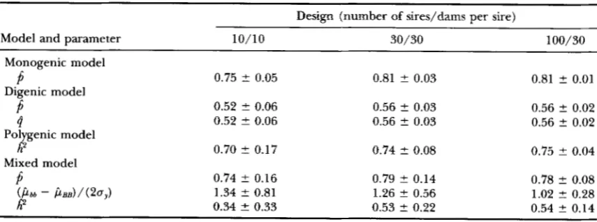
Average parameter estimates and empirical standard errors; true state: mixed model; major gene effect of 1.0

Monogenic model

Digenic model

P

0.75 t 0.05 0.81 ? 0.03 0.81 ? 0.01

P

0.52 2 0.06 0.56 2 0.03 0.56 ? 0.02

4

0.52 2 0.06 0.56 ? 0.03 0.56 ? 0.02

ff

0.70 t 0.17 0.74 ? 0.08

P

0.74 5 0.16 0.79 t 0.14 0.78 2 0.08

Polygenic model

Mixed model 0.75

? 0.04

h2

( b b b - P B B ) / (207) 1.34 5 0.81 1.26 2 0.56 1.02 2 0.28

(8)

1826 G . Thaller, L. Dempfle and I. Hoeschele

TABLE 9

Average parameter estimates and empirical standard errors; true state: mixed model; major gene effect of 2.0 a,

Monogenic model

Digenic

P

model 0.80 t- 0.05 0.85 +- 0.02 0.85

*

0.01

P

0.59 2 0.13 0.65 ? 0.06 0.64 ? 0.03

4^

0.50 t- 0.15 0.55 +- 0.11 0.58 +- 0.05

h-2 0.78 2 0.10 0.80 ? 0.00 0.80 ? 0.00

P

0.79 ? 0.09 0.80 ? 0.02 0.80 ? 0.01

e

Polygenic model

Mixed model

( b b b - bBB)/(2'y) 2.10 ? 1.02 2.19 +- 0.54 2.13 t- 0.29

0.31 ? 0.33 0.56 ? 0.21 0.52 ? 0.12

polygenic model. Under the mixed model, allele frequency at the major locus was estimated accurately, in particular for the largest design. Homozygote difference still tended to be overestimated, although not sig- nificantly due to its large standard error. As a conse- quence, variance VG at the major locus overestimated the true value of 3.686 by attaining values of 4.138 and 4.181 for the smallest and largest design, respectively. Polygenic heritability was underestimated only for the smallest design and its standard errors decreased substantially with increasing design size.

In general, the parameter estimates were helpful in interpreting the results on hypothesis testing in Table 3. Under the true monogenic model, the maximized likelihoods for the monogenic, digenic and mixed models were nearly identical. This can be explained by the allele frequency estimate near zero in the digenic model and the extremely large estimate of the homozygote difference in the mixed model, virtually turning the digenic and mixed models into the monogenic model. Under the true digenic model, the maximized likelihoods for the digenic and mixed models of analysis were very close. Based on the parameter estimates from the mixed model, the effects of the two loci were explained both with the major locus and with polygenic heritability, at least for the largest design.

Extreme category problem: When data were simulated under the monogenic model of inheritance, all individuals homozygous for the recessive allele ex- pressed the disease. When these data were analyzed with the mixed model, the extremely high estimate of the homozygote difference at the major locus caused the mixed likelihood to mimic the monogenic likelihood, where genotype perfectly determines outcome (affected or unaffected). Even when the mixed model is the true state of nature rather than the monogenic model, for certain parameter combinations (e.g., those used in the simulation of the A data sets) it can happen by chance that all recessive homozygous individuals ex- hibit the disease, despite the polygenic background.

That is, in a given sample of data, major genotype determines outcome. To see whether this situation can be distinguished from the monogenic case by the analysis, several A data sets were simulated, and those where all affected individuals were homozygous recessive at the major locus were retained and analyzed.

In the general context of analysis of categorical data, the so-called extreme category problem (ECP) (MIS

ZTAL and GIANOLA 1989) occurs when there is no variation in the observed data within a level of a fixed factor (here, genotype). If all observations on a binary trait within the same level of a fixed effect fall into the same category of response ( 0 or l ) , the estimate of this fixed effect will drift toward - or

+

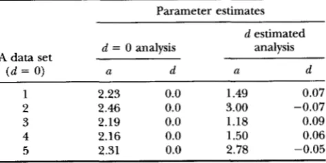
infinity, and convergence of the estimation procedure does not occur. Hence, if the genotypes of all individuals were known and all animals homozygous for the recessive major gene increasing the incidence of the defect were affected, then the genotypic deviation for this genotype cannot be estimated.

The A data sets were simulated both with d = 0 and with d = -a, and were analyzed first with these restrictions and second by estimating parameters a and d freely. Results for the data sets simulated with d = 0 are in Table 10. Parameter a was well estimated with d fixed

TABLE 10

Parameter estimates for major gene and dominance effect when analyzing A data sets with ECP generated under d = 0

Parameter estimates

d estimated analysis

d = 0 analysis

A data set

( d = 0) U d U d

1 2.23 0.0 1.49 0.07

2 2.46 0.0 3.00 -0.07

3 2.19 0.0 1.18 0.09

4 2.16 0.0 1.50 0.06

(9)

Inheritance of Rare Binary Traits 1827

TABLE 11

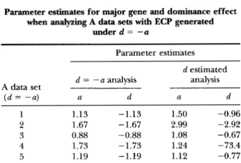
Parameter estimates for major gene and dominance effect when analyzing A data sets with ECP generated

under d = --a

Parameter estimates

d estimated

A data set d = - a analysis analysis

( d = -a) a d a d

1 1.13 -1.13 1.50 -0.96

2 1.67 - 1.67 2.99 -2.92

3 0.88 -0.88 1.08 -0.67

4 1.73 - 1.73 1.24 -73.4

5 1.19 -1.19 1.12 -0.77

at the true value of zero, because the difference in the affectedness of BB and Bb animals ( b being the recessive allele) is sufficient to estimate a. However, estimates of

a and d were inaccurate and very variable when d was also estimated, although the estimate for a did not drift toward infinity. This result can be explained by the analysis considering the genotypes of at least some bb

individuals as uncertain, while under the monogenic model estimates of a drifted toward infinity, because the analysis did not attach any uncertainty to the genotypes of bb individuals. Analyzing data sets generated with d = - a (Table 11) resulted in unreliable estimates for a (although these did not drift toward infinity), even if d was fixed at the true value, because there was no variation between BB and Bb genotypes in affectedness. Parameter estimates under the true mixed model were generally quite accurate in the absence of the ECP (Tables 7-9). If large variability among major gene parameter estimates from different subsets of data or from different starting values are observed in practice, this finding may be caused by all individuals of the extreme genotype falling into the same category of response.

Power and robustness: Empirical distributions of the likelihood ratio test statistic were derived by simulation, with 100 replicates for design 10/10 and 50 replicates for designs 30/30 and 100/30. Results on empirical distributions were obtained with the monogenic and with the polygenic model as the null hypothesis. The data sets analyzed were generated under the respective null hypothesis. Characteristics of the distributions ex- amined were mean, standard deviation and 95% quan- tile. The 95% quantiles were obtained by sorting the 100 (or 50) Tvalues obtained for each design and null hypothesis and finding the smallest Tvalue among the upper 5% of all Tvalues. The empirical 95% quantiles were then used to evaluate the power of the tests and will be referred to as significance thresholds at the 0.05 type-I error level or T ~ % .

The results in Table 12 are based on the monogenic model as the null hypothesis. For testing the digenic against the monogenic model, if one would incorrectly assume asymptotic theory to hold, one would expect a

TABLE 12

Properties of test statistics for the monogenic model

as the null (true) hypothesis

Design

(number of sires/dams per sire)

Alternative model 10/10 30/30 100/30

Digenic model

P

0.34 -0.27 -2.23

B 1

.oo

1.58 4.25

7 5 % 1.89 2.30 2.64

P

-18.75 -159.16 -527.00

B 9.60 37.35 51.48

7 5 % -3.38 -85.38 -434.53

P

0.44 0.07 0.001

b 1.36 0.48 0.0002

7 5 % 3.50 0.06 0.0014

Polygenic model

Mixed model

Means, standard deviations and empirical thresholds for Type I error of 5%.

chi-squared distribution with mean 1, standard deviation of 1.41 and 95% percentile of 3.84. The empirical distribution is in clear disagreement with these expecta- tions. The polygenic and monogenic models are nonnested models for which the likelihood ratio test is not applicable, i e . , the distribution of the differences in log likelihood values must always be found empirically.

The results for testing the mixed us. the monogenic model confirmed again that the mixed likelihood a p proaches the monogenic likelihood, when the monogenic model is the true model. The empirical mean of the likelihood ratio statistics was low and approached zero for the largest design with very small standard deviation.

The results in Table 13 are based on the polygenic

TABLE 13

Properties of test statistics for the polygenic model

as the null (true) hypothesis

Design

(number of sires/dams per sire)

Alternative model 10/10 30/30 100/30

Monogenic model

F

-53.52 -479.46 -1569.48

b 15.08 32.07 64.25

7 5 % -28.77 -421.64 -1476.73

P

-16.49 -134.34 -441.94

b 7.95 22.27 41.82

7-5% -6.05 -100.19 -370.45

P

0.59 1.15 1.22

b 1.28 3.99 2.68

7 5 % 3.31 5.03 8.18

Means, standard deviations and empirical thresholds for

Digenic model

Mixed model

(10)

1828 G. Thaller, L. Dempfle and I. Hoeschele

TABLE 14

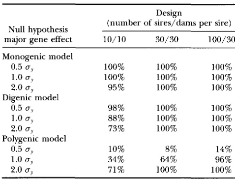
Power of the methodology for accepting the true mixed model compared with the monogenic, digenic

or polygenic model as the null hypothesis

Design

(number of sires/dams per sire) Null hypothesis

major gene effect 10/10 30/30 100/30

Monogenic model

0.5 os 100% 100% 100%

1.0 uy 100% 100% 100%

2.0 oJ 95% 100% 100%

1.0 uy 88% 100% 100%

2.0 o? 73% 100% 100%

1.0 0, 34% 64% 96%

2.0 uy 71 % 100% 100%

Digenic model

0.5 0 , 98% 100% 100%

Polygenic model

0.5 uy 10% 8% 14%

model as the null hypothesis. Again, testing the monogenic and digenic models against the polygenic model involves nonnested models. Mean values for Twere neg- ative and in favor of the true model. The digenic model performed better than the monogenic model as it represents a first step toward the infinitesimal model. The likelihood ratio statistic for the mixed us. the polygenic model does not have an asymptotic chi-squared distribution with degrees of freedom equal to the difference in the number of parameters, although these are nested models. Although the mixed model includes two additional parameters, restriction of only one parameter

( p

= 0 or a = 0) leads to the polygenic likelihood. Both restrictions are at the boundary of the parameter space. Furthermore, given that

p

= 0, the likelihood will be constant for all values of a and vice versa. Therefore, the mixed likelihood will never approximate the shape of a full-rank normal density, even with very large sample sizes, and hence the asymptotic theory is invalid

(e.g., TITTERINCTON et al. 1985).

To evaluate the power of the methodology, data were simulated under the alternative hypothesis. The frac- tion of T values exceeding the threshold value ( T ~ % )

was an estimate of the power for rejecting the null hypothesis. The threshold values were the 7 5 % values in

Tables 12 and 13, and additional T ~ % values were determined analogously for the digenic model as the null hypothesis. Table 14 shows the power for rejecting the null hypotheses equal to the monogenic, digenic and polygenic models in favor of the mixed model. Very high power was achieved for testing the mixed vs. the oligogenic and digenic models, i e . , testing for variation within major genotype. For the smallest design, however, power appeared to decrease with increasing major gene effect.

The power of testing for a major gene in addition to polygenic inheritance (mixed model vs. polygenic

model) was poor for a major gene effect of half of a standard deviation across designs. The power of de- tecting a major gene with an effect of one standard deviation depended strongly on the design, with acceptable power being found for design 30/30 and very high power for design 100/30. For a major gene effect of two standard deviations, power was high in all three designs.

Power estimates for comparisons between the polygenic and the monogenic models were always equal to 1 and are not presented here. Overall, the methodology provided satisfactory power for distinguishing between the modes of inheritance postulated for a rare binary trait and practical designs.

Conclusions: Complex segregation analysis of binary traits by ML, based on the infinitessimal mixed model, with deterministic algorithms is computationally feasible when assuming no relationships among parents and no additional random or fixed effects. Numerical algorithms for integrating and maximizing the likelihood function were efficient even for a design with 100 sires and 30 dams per sire. The result of computational feasi- bility holds only for analyses of individual data sets. Performing hypothesis testing based on the distribution of the test statistic under the null hypothesis is computationally prohibitive, because the distribution must be found empirically by simulation or data permutation, as asymptoptic theory does not hold for comparisons among oligogenic, polygenic and mixed models. Ob- taining reliable empirical threshold values for the likelihood ratio via simulation or data permutation would likely require a large number of replicates or permuta- tions, respectively, e.g., 1000.

Despite these difficulties in hypothesis testing, the results on model choice via the AIC were encouraging, as almost always the correct model was chosen based on this criterion. The only exception occurred for the mixed model with the smallest major gene effect, where the polygenic model was chosen as the best model by the AIC in all designs. Based on the results obtained in this study, major genes with half of the homozygote difference equal to at least one standard deviation (within major genotype) of the underlying liability of a rare binary trait can be detected in practice. TO the authors' knowledge, previous applications of complex segregation analysis in animal genetics all dealt with continuous traits, where the lower limit for detection of a major gene was also equal to one standard deviation of the within-genotype variation (e.g., KNOTT et al.

(11)

Inheritance of Rare Binary Traits 1829

couraging. In particular, data sets simulated under the mixed model were fitted poorly with the monogenic and digenic models, allowing the animal breeder to detect and utilize both major locus and polygenic variance if these coexist.

To demonstrate that major genes with an effect of one standard deviation could exist in actual data ( . g . , THALLER et al. 1996), consider a hypothetical example with an overall disease incidence of 1%, frequency of the recessive homozygotes of 4%, disease incidence of 20% in the recessive homozygotes and of 0.2% in the remaining population. This difference in incidence between the two populations corresponds to a difference in means in the liability scale of near 2 standard deviations. In an analysis of actual data (THALLER et al. 1996), litter variance was fitted as an additional parameter. However, it was not fitted in the simulation study because the increase in CPU time would not have permit- ted sufficient replication of the designs studied here. We do not believe that the inclusion of a litter effect would have affected the conclusions arrived at here. However, fitting litter variance in real data analyses is obligatory, as it could incorrectly indicate the presence of a major gene.

Further improvements in the detection of single genes can be expected when genetic markers and ade- quate statistical methods to utilize this information are available. Although only very small numbers of animals need to be genotyped when using homozygosity mapping (LANDER and BOTSTEIN 1986) to locate a major recessive gene, much larger numbers of individuals are needed for parameter estimation and to distinguish between oligogenic, polygenic and mixed modes of inheritance. With phenotypic observations abundantly available, our methodology is a worthwhile first step in identifying mode of inheritance and single genes affect- ing binary traits of economic importance in livestock.

Two avenues can be followed to accommodate the utilization of all the available pedigree information, which are the application of Markov chain and Monte Carlo algorithms to ML (e.g.,

Guo

and THOMPSON 1992) or Bayesian complex segregation analysis (we will be reporting on this in a separate communication), or complex segregation analysis based on the finite polygenic mixed model of FERNANDO et al. (1995). To accommodate a large number of additional nuisance parameters (fixed effects, variance components), a Bayesian approach seems more suitable than ML, because it can account for uncertainty associated with the nuisance parameters and incorporate prior information, if available.

G. T. acknowledges financial support from the Technische Uni- versiat Mfinchen-Weihenstephan, Germany, and the Deutsche Forschungsgemeinschaft DFG. I.H. acknowledges support from the U.S. National Science Foundation (grant no. BIR-9407862) and from the European Human Capital and Mobility Fund while on research leave at Wageningen University, The Netherlands.

LITERATURE CITED

ABRAMOWTZ, M., and J. A. STEGUN, 1970 Handbook of Mathematical Functions. Dover Publication, Inc., New York.

AKAIKE, H., 1973 Information theory and an extension of the maximum likelihood principle, in Second International Symposium on Information, edited by B. N. PETROV and F. CSAKI. Akademia Kiado, Budapest, Hungary.

CHURCHILL, G. A,, and R. W. DOERGE, 1994 Empirical threshold values for quantitative trait mapping. Genetics 138: 963-971.

CURNOW, R. N., 1984 Progeny-testing for all-or-none traits when a multifactorial model applies. Biometrics 40: 375-382.

ELSTON, R. C., and J. STEWART, 1971 A general model for the genetic analysis of pedigree data. Hum. Hered. 21: 523-542.

FALCONER, D. S., 1986 Introduction to Quantitative Genetics, Ed. 3.

Longman Scientific & Technical, New York.

FERNANDO, R. L., C. STRICHER and R. C. ELSTON, 1994 The finite polygenic mixed model: an alternative formulation for the mixed model of inheritance. Theor. Appl. Genet. 88: 573-580.

GIANOLA, D., and J. L. FOULLEY, 1983 Sire evaluation for ordered categorical data with a threshold model. Genet. Sel. Evol. 15:

201-223.

Guo, S. W., and E. A. THOMPSON, 1992 A Monte Carlo method for combined segregation and linkage analysis. A m . J. Hum. Genet. 51: 1111-1126.

HARTL, D. L., and T. MARUYAMA, 1968 Phenograin enumeration: the number of regular genotype-phenotype correspondences in genetic systems. Theor. Biol. 2 0 129-163.

HENDERSON, C. R., 1976 A simple method for computing the inverse of a numerator relationship matrix used in prediction of breeding values. Biometrics 32: 69-83.

HILL, W. G., and S. A. W o n , 1990 Detection of genes of large effect, pp. 517-537 in Advances in Statistical Methods for Genetic Improvement oflivestock, edited by K. H A ” O N D and D. GIANOIA. Springer Verlag, Berlin.

HOESCHELE, I., 1988 Genetic evaluation with data presenting evi- dence of mixed major gene and polygenic inheritance. Theor. Appl. Genet. 76: 81-92.

HOESCHELE, I., GIANOLA, D. and J. L. FOULLEY, 1987 Estimation of variance components with quasi-continuous data using Bayesian methods. J. Anim. Breed. Genet. 104 334-349.

JANSS, L. L. G., THOMPSON, R. and J. A. M. van AFENDONK, 1995

Application of Gibbs sampling for inference in a mixed major gene-polygenic inheritance model in animal populations. Theor. Appl. Genet. 91: 1137-1147.

S. A,, and C. S. HALEY, 1992 Maximum likelihood mapping of quantitative trait loci using full-sib families. Genetics 132:

1211-1222.

KNOTT, S. A., HALEY, C. S. and R. THOMPSON, 1991a Methods of segregation analysis for animal breeding data: a comparison of power. Heredity 6 8 299-31 1.

KNOm, S. A., HALEY, C. S. and R. THOMPSON, 1991b Methods of segregation analysis for animal breeding data: parameter estimates. Heredity 68: 313-320.

LANDER, E. S., and D. BOTSTEIN, 1986 Mapping complex genetic traits in humans: new methods using a complete RFLP linkage map. Cold Spring Harbor Symp. Quant. Biol. 2: 49-62.

MISZTAL, I., and D. GIANOLA, 1989 Computing asDects of a nonlin- ear method of sire evaluation for citegoryal data. J. Dairy Sci.

72: 1557-1568.

MORTON, M. E., and C. J. MCLEAN, 1974 Analysis of family resem- blance. 111 Complex segregation analysis of quantitative traits.

A m . J. Hum. Genet. 26: 489-503.

NAYLOR, J. C., and A. F. M. SMITH, 1982 Applications of a method for the efficient computation of posterior distributions. Appl. PRESS, W. H., B. P. FLANNERY, S. A. TEUKOLsKYand W. T. VETTERLING,

1986 Numerical recipes-the art of scientific computing. Cam- bridge University Press, Cambridge.

THALLER, G., L. DEMPFLE and I. HOESCHELE, 1996 Investigation of the inheritance of birth defects in swine by complex segregation analysis. J. Anim. Breed. Genet. 113: (in press).

TITTERINGTON, D. M., A. F. M. SMITH, and U. E. MAKOV, 1985 Statisti- cal analysis of finite mixture distributions. John Wiley & Sons, New York.

WADA, Y, and N. KASHIWAGI, 1990 Selecting statistical models with information statistics. J. Dairy Sci. 73: 3575-3582.

Stat. 31: 214-225.

Maximum Likelihood Analysis of Rare Binary Traits Under Different Modes of Inheritance