The complex-step method for sensitivity analysis of
non-smooth problems arising in biology
H.T. Banks, Kidist Bekele-Maxwell, Lorena Bociu,
Marcella Noorman, and Kristen Tillman
Center for Research in Scientific Computation
Department of Mathematics
North Carolina State University
Raleigh, NC 27695-8212
October 15, 2015
Abstract
We investigate the complex-step method as applied to compute sensitivities with respect to model “parameters” for several types of examples. We first consider time delayed differential equations (DDEs) whose sensitivities are known to have lack of smoothness or even discontinuities with respect to parameters such as the delays. The second type of “parameter sensitivity” we consider is that of solutions to partial dif-ferential equations (PDEs) with respect to boundary conditions which again may not possess smoothness. These sensitivities are fundamental in any type of boundary con-trol formulation such as those we motivate in Section 4 below.
Our main focus here is to evaluate the so-called “complex-step methods” for com-puting such sensitivities. This is of interest since the complex-step method was derived based on the Cauchy-Riemann equations for analytic complex functions. Our compu-tational findings are compared to those using the standard chain rule-based sensitivity differential equations which can be rigorously developed even for derivatives possessing much less regularity than analyticity. Our findings suggest that the complex-step meth-ods are in very good agreement with the usual sensitivity equation results up to some critical step size we callhcrit. They can offer significant savings in computational costs
for problems driven by complicated dynamical systems with reasonable parameter size.
1
Introduction
Sensitivity analysis continues to play a fundamental role in modeling, mathematics, statistics and engineering for an incredibly wide range of applications. This topic plays a critical role in widely diverse topics including:
• parameter selection and identifiability [11] and many references therein, [6, 9] in inverse problem formulations;
• statistics and Fisher Information Matrix [13, 25, 34, 35, 62], and in particular asymp-totic theories for large sample size problems;
• data set information content studies [12];
• optimal design of experiments [22, 23];
• PDEs and boundary term sensitivity [19, 21] as potential control formulations in biomedical studies–see, for example, recent references on modeling pathologies such as glaucoma in the human eye [26, 32, 37, 42]; such studies are precursors to general boundary control design which are also often studied in a wide range of engineering problems;
• non-smooth problems where one does not have analyticity of response with respect to the “parameters”, including delay systems with respect to delays [24], where the usual situation is represented by a lack of smoothness, let alone analyticity; and PDE prob-lems with respect to boundary parameters such as those in aggregate data probprob-lems where estimated parameters are probability measures [13, Chapter 6] and the examples and references therein.
In usual sensitivity analyses, one studies how the output of a model is affected by a wide variety of inputs. In these efforts we are concerned with calculating the rates of change in the output variables (solutions or observables) of a system which result from small perturbations in the problem parameters.
We outline an ODE inverse problem framework to illustrate the basic ideas even though we will be concerned with more complicated systems and sensitivities to delays in a DDE and to boundary inputs in PDE formulations. Consider an n-dimensional vector system
dx
dt =g(t,x(t),q) (1.1)
x(t0) =x0
with observation process (we assume without loss of generality a scalar observation process)
f(t;θ) =Cx(t;θ),
whereθ = [qT,x
in notation we do not-see [13, 25] for such more general formulations). The inverse problem is to determineθ using given observations over time. Using an ordinary least-squares method (OLS) for estimation (again, more general formulations can be found in [13, 25]), we wish to find
ˆ
θOLS= arg min
θ∈Ωθ
n
X
j=1
(yj −f(tj;θ))2
where yj is the data at time tj and Ωθ is the admissible set for the parameters.We assume that ˆθOLS follows a normal distribution with meanθ0 and covariance matrix Σ0 ≈σ20[χTχ]
−1
where
χjk =
∂f(tj;θ)
∂θk
(1.2)
The matrix χ is called the sensitivity matrix. Our goal is to compute ∂f(tj;θ)
∂θk as efficiently
and accurately as possible. There are various ways of approximating these derivatives. The most common ones (see [18, 13, 25] and the references therein) are analytic methods, finite difference approximation, automatic differentiation and the use of sensitivity equations. Analytic methods are accurate but they require the derivation and development of a program that is specific to each problem, hence inefficient. The finite difference method, on the other hand, is relatively easy and efficient to implement but it suffers from cancellation error. Sensitivity equations are known to be accurate and computationally inexpensive for reasonably small systems.
More recently, a method referred to as the complex-step has been used to calculate sen-sitivities ([55, 56]). The idea of using complex variables to estimate derivatives originated with the work of Lyness and Moler [52] and Lyness[51]. After its rediscovery by Squire and Trapp in 1998, it has become quite popular in aerodynamic optimization [1, 2, 55, 56, 65]. The complex-step estimate is suitable for use in numerical computing and shown to be very accurate, extremely robust while retaining a reasonable computational cost. Martins, et al., in [55] have shown the method to have implementation advantages over automatic differenti-ation and computdifferenti-ational advantages over finite-differencing. Although a step size parameter is required, in most cases the numerical derivatives are not subject to subtractive cancellation errors as in the use of finite differences, (see [56] for exceptions and remedies). Therefore, the method exhibits true second-order accuracy as the step size is reduced. In addition, the procedure is easily implemented into existing programs. The only requirements are that the floating point variables be declared as complex and that a complex perturbation be added to the variable of interest.
2
The complex-step method
In this section, following [55], we summarize the complex-step method. Given (1.1), let
z = x+iy, x, y ∈ R be a complex number and f(z) = f(x, y) = u(x, y) +iv(x, y) be a function of a complex variable. If f is analytic, we have the following Cauchy-Riemann equations that establish the relationship between the real and imaginary parts of the function.
∂u
∂x(x, y) = ∂v ∂y(x, y),
∂u
∂y(x, y) = − ∂v
∂x(x, y) (2.1)
For a given step size h we can derive a finite difference-like first derivative estimate for real functions using complex calculus. From the first equation in (2.1), and the definition of derivatives we have
∂u
∂x(x, y) = limh→0
v(x, y+h)−v(x, y)
h (2.2)
= lim h→0
Im[f(x+i(y+h))]−Im[f(x+iy)]
h . (2.3)
If f takes a real-valued input (as in the case where, for example, f represents the solution to a differential equation model), then y = 0, f(x) = u(x,0), and v(x,0) = Im[f(x)] = 0. Thus (2.2) becomes
∂f
∂x = limh→0
Im[f(x+ih)]
h . (2.4)
Therefore, for small h, we have the complex-step derivative approximation
∂f ∂x ≈
Im[f(x+ih)]
h . (2.5)
This formula can also be obtained by approximating an analytic functionf with a complex variable using a Taylor series expansion:
f(x+ih)≈f(x) +ihf0(x)− h
2
2!f 00
(x)−ih
3
3!f
(3)
(x) + h
4
4!f
(4)
(x) +· · ·
Taking the imaginary parts of both sides and dividing by h gives
f0(x)≈ Im[f(x+ih)]
h +O(h
2).
Terms of order h2 and higher can be ignored because the step size h can be chosen up to
machine precision. Thus the complex-step derivative is given by (2.5) with a truncation error
Et(h) = h
2
6 f
(3)(x). The method is accurate down to a specific step size we call h
crit. Below
The derivative estimate (2.5) constitutes a big advantage over the finite-difference ap-proach. This is because the finite-difference approximation is subject to subtractive error due to the differencing operation. On the other hand, the accuracy of the complex-step esti-mates is only limited by the numerical precision of the algorithm that evaluates the function
f.
Note that the complex-step approximation formula (2.5) is derived based on the Cauchy-Riemann formula for analytic functions. Therefore, it is important that the function f be analytic. In the case when the functions have singularities or branch cuts where they are not analytic, the complex-step method provides a correct derivative approximation up to the point of discontinuity. In addition, we get accurate approximations of one-side derivatives if we uniquely define the function at that point. The method also provides an accurate first order derivative when a function has jumps in its higher order derivatives (see examples 4.2-4.4).
2.1
Implementation
2.1.1 Complex function definitions
The complex-step approximation formula (2.5) is derived based on the Cauchy-Riemann formula assuming the function f is analytic. Then it is important to investigate to what extent this assumption holds when the value of the function is calculated by a numerical algorithm. In addition we need to extend functions of real variables to complex in such a way that the Cauchy-Riemann equations are satisfied. Even though our discussion below is for implementation of the complex-step in Matlab, the principles are the same for other programming languages. For further discussion and Fortran implementation, we refer the reader to [55] and [56] .
When we convert a ‘real’ algorithm to complex, we are mainly concerned with two types of operations:
1. Relational operators
Relational logic operators like “greater than” and “less than” are defined in Matlab to compare only the real parts of a complex number. These operators are usually used in ‘if’ statements to redirect the execution thread. The original algorithm and its complex version must follow the same execution thread. Therefore, the Matlab definition of these operators is the correct one.
2. Arithmetic functions and operators
In Matlab, complex numbers are a standard data type and many functions have com-plex counterparts. Functions that choose one argument like max and min are based on relational operators. Therefore, one would assume that they are defined based on their real parts in Matlab. Unfortunately, that is not the case. In Matlab, min and
max functions compare the radii of two complex numbers. Hence, they need to be redefined to compare only the real parts.
Another function that we need to give attention to is the absolute value (abs) function.
definition was not derived assuming the Cauchy-Riemann equations, the complex-step method does not give a correct derivative approximation. Therefore, we need to define ‘abs’ so that it satisfies the Cauchy-Riemann equations. Since we know what the value of the derivative must be, we can write
∂u ∂x =
∂v ∂y =
−1, x <0
+1, x >0 (2.6)
From (2.1), since ∂v/∂x = 0 on the real axis, we get ∂u/∂y = 0 on the same axis, so the real part of the result must be independent of the imaginary part of the variable. Therefore, the new sign of the imaginary part depends only on the sign of the real part of the complex number, and an analytic absolute value function can be defined as:
abs(x+iy) =
−x−iy x <0
x+iy x≥0 . (2.7)
This function is not analytic atx= 0. But, as was mentioned earlier, the complex-step approximation yields an accurate derivative up to the discontinuity. In addition, since we have defined the function at x = 0 as for x > 0, the method gives the correct right-hand side derivative atx= 0.
Similarly, for every real valued function, by requiring that its complex extension satis-fies the Cauchy-Riemann equations, and that the real and the complex have the same properties, we can obtain a unique complex function definition either by adjusting the definition of custom functions, or ensuring that Matlab’s complex analog function is correctly defined.
Many of the arithmetic operators including addition, multiplication, and trigonometric function have standard complex definitions that are analytic almost everywhere.
The transpose (·) operator in Matlab gives the complex conjugate of the matrix. So we need to use the non-conjugate transpose (·0) instead.
We remark that before implementing the complex-step method, one always needs to check whether the functions and operators in the algorithm need re-definition and do so accordingly.
2.1.2 Implementation Procedure
Given an analytic functionf, the following is an outline of the general steps for implementing the complex-step method for computing the first derivative, df /dx.
2. Add a small complex stepihto the desired variable ‘x’, run the algorithm that evaluates
f.
3. Compute df /dxusing (2.5).
2.2
Generalization for vector-valued functions
Given a step size h, and the vector valued function f : Rn →
Rm which takes the vector
x∈Rnand produces the vectorf(x)∈
Rm, the complex-step approximation of the Jacobian
matrix is given by [50]
J ≈1
hIm
f1(x+ihe1) · · · f1(x+ihej) · · · f1(x+ihen)
..
. ... ...
fp(x+ihe1) · · · fp(x+ihej) · · · fp(x+ihen) ..
. ... ...
fm(x+ihe1) · · · fm(x+ihej) · · · fm(x+ihen)
(2.8)
3
Sensitivity Equations
In this section, we briefly summarize the derivation of sensitivity equations for the ODE model (1.1) which can be extended for PDEs in a similar way. For extensive discussion of the method, see [13] and [18] and references therein.
Given (1.1), first we derive sensitivity equations for the parameterq. Lets= (sq1,· · · ,sqk),
where
sqk(t) =
∂x
∂qk
(t;θ), k = 1,· · · , p. (3.1) Taking the derivative of equation (1.1) with respect toq, we obtain
ds(t)
dt = ∂g
∂xs(t) +
∂g
∂q (3.2)
s(t0) = 0n×p.
For the initial conditionx0, let r = (rx01,· · · ,rx0n) where
rx0j(t) =
∂x
∂x0j
(t;θ), j = 1,· · · , n. (3.3) Then we obtain the system
dr(t)
dt = ∂g
dxr(t) +
∂g
∂x0
(3.4)
= ∂g
∂xr(t), r(t0) =In×n.
To find sensitivities, we solve equations (3.2) and (3.4) together with (1.1). Namely, we solve
dx(t)
dt =g(t,x(t),q), ds(t)
dt = ∂g
∂xs(t) +
∂g
∂q,
dr(t)
dt = ∂g
∂xr(t), x(t0) = x0,
s(t0) = 0n×p,
4
Numerical Examples
In this section, we apply the complex-step method to compute sensitivities for various kinds of examples and we compare the results with solutions of sensitivity equations ( or analytic solutions when available). The first example is the logistic model for population growth which is a simple enough ODE model yet a widely applied example in biological applications [48, 60]. This simple example can be used to calibrate our computational times.
We then turn to two classes of examples where the underlying foundations for the complex step method do not hold. The first of these is delay differential (also called functional
differential) equations where sensitivity with respect to the delays or hysteresis kernels do
not in general satisfy the analyticity requirements for use of the Cauchy-Riemann equations. Delay equations have been used in a wide variety of biological applications as well as in many engineering problems –see for examples the references [3, 4, 7, 8, 27, 28, 29, 30, 33, 36, 38, 39, 40, 41, 43, 45, 49, 53, 54, 61]. Very early interest in the 1940’s focused around the studies of mechanical systems by Minorsky [57, 58, 59] and slightly later those of Hutchinson [46, 47] in biology. Both of these authors argued that time delays in dynamical systems can produce oscillatory phenomena in an otherwise non-oscillatory system.
In 1948 Hutchinson [46] developed a delay differential equation model, subsequently known as Hutchinson’s equation, which is the delayed logistic equation, to describe the dy-namics of a circular causal system. An example of an ecological circular causal system is a parasite-host interaction where a parasite completes its life cycle without killing the host or drastically altering the growth of the host population. The host population can then continue to exist [46, 49]. The delay in this model can represent various naturally occurring phenomena such as the gestation period in a growing population, the life cycle of a parasite, cell cycle delays, etc. Hutchinson’s equation (to be used along with Minorsky’s harmonic oscillator with a delayed damping in the numerical illustrations below), its variations and other delay systems have also been used to model physiological control systems as well as numerous other biological processes.
Delay differential equations (DDEs) are particularly interesting because the derivatives of their solutions often have discontinuities (see [24] for a theoretical treatment and discussions). This is generally true because the first derivative of a non-constant history function at zero is almost always different from the right derivative of the solution at the initial point. As we shall see below, in addition to the discontinuity at the initial point, discontinuities in derivatives of the initial function tend to be propagated with one degree of smoothness added per time delay interval. Since the complex-step method is derived assuming analyticity, one would expect for the method to fail when it comes to computing the sensitivity with respect to the time lag τ. But the results for these examples show that the complex-step method approximates the sensitivities accurately up to hcrit even in the presence of discontinuities in the solutions.
the perfusion of the lamina cribrosa in the optic nerve head. Retinal hemodynamics plays a crucial role in the pathophysiology of several ocular diseases, including glaucoma, age-related macula degeneration and diabetic retinopathy. The retinal vascular bed nourishes the retinal ganglion cells that are responsible for the transmission of visual information from the retina to the brain, via the optic nerve. Blood is supplied by the central retinal artery (CRA), and drained by the central retinal vein. The central retinal vessels, i.e., central retinal artery and vein, run through the optic nerve canal, where they are exposed to the retrolaminar tissue pressure (RLTp). They also enter inside the eye globe, where they are exposed to the intraocular pressure (IOP). The pressure difference between the RLTp in the optic nerve tissue (baseline value 7-10 mmHg) and the IOP inside the eye globe (baseline value 12-15 mmHg) is maintained by the lamina cribrosa, a collagen structure that is pierced by the central retinal vessels approximately in its center. There are clear evidences that the CRA hemodynamics is strongly affected by the level of IOP inside the eye globe. Control of the IOP leads to a natural optimization problem involving boundary control of a PDE system (a linear poroelastic system). Again in general one does not expect analyticity of the Dirichlet or Neumann BC map to the solution. Here we investigate performance of the complex-step method in computing the relevant sensitivities. Again, in comparing the sen-sitivity equations results to those using the complex-step method, we find good agreement up to somehcrit which suggests that the complex-step method performs well even when the model at hand is more sophisticated and lacks the appropriate analyticity requirements of the boundary-to-solution maps.
4.1
The logistic model for population dynamics
In traditional population growth model, as developed by Malthus (1798), the growth rate is proportional to the size of population:
dx(t)
dt =rx(t)
wherer is the intrinsic growth rate of the population andx(t) represents the population size at timet. As a result, the population grows exponentially:
x(t) =x0ert,
wherex0 =x(0) is the initial population. In reality, this model may only be valid for a short
time period because the environment imposes limitations to population growth. A more accurate model by Verhulst (1836) postulates that the relative growth rate approaches the
carrying capacity K of the environment. The corresponding equation is called the logistic
differential equation:
dx(t)
dt =rx(t)
1− x(t)
K
, 0< t≤T (4.1)
with analytic solution
x(t) = K 1 +xK
0 −1
ert
.
We compute the sensitivities of the solutionxwith respect to the parametersr, K, x0 using
both the complex-step method and sensitivity equations.
0 5 10 15 20 25
0 2 4 6 8 10 12 14 16 18
Time
x(t)
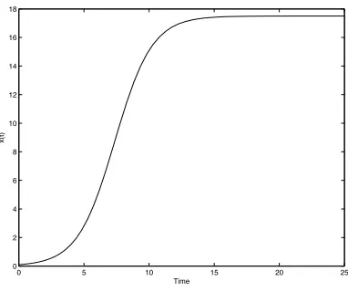
Figure 1: Solution function of the logistic equation atr = 0.7, K = 17.5, x0 = 0.1.
To derive the sensitivity equations, we take the derivative of the equation with respect to each parameter. The sensitivity equations are, thus, given by
dx(t)
dt =rx(t)
1− x(t)
K
, dsr(t)
dt =
r−2r
Kx(t)
sr(t) +x(t)− 1
Kx
2
(t), dsK(t)
dt =
r−2r
Kx(t)
sK(t) + r
K2x 2
(t), dsx0
dt =
r−2r
Kx(t)
sx0(t),
with initial conditions
x(0) =x0, sr(0) =sK(0) = 0, sx0(0) = 1.
where sK(t) = ∂x∂K(t), sr(t) = ∂x∂r(t), sx0(t) =
∂x(t)
∂x0 .
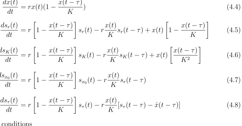
In Figure 2 below, we compare the sensitivity functions computed by solving the above sensitivity equations and the complex-step method. As it is shown, the accuracy of the complex-step approximation starts to decline at hcrit = 10−320. We have displayed the sensitivities at h = 10−40 and at h = 10−321 side by side. (Recall our machine accuracy is 10−324).
0 5 10 15 20 25
0 5 10 15 20 25 30 35 x r(t) complex−step sensitivity equations
0 5 10 15 20 25
0 5 10 15 20 25 30 35 x r(t) complex−step sensitivity equations
0 5 10 15 20 25
0 0.1 0.2 0.3 0.4 0.5 0.6 0.7 0.8 0.9 x K(t) complex−step sensitivity equations
0 5 10 15 20 25
0 0.1 0.2 0.3 0.4 0.5 0.6 0.7 0.8 0.9 1 x K(t)
complex−step sensitivity equations
0 5 10 15 20 25
5 10 15 20 25 30 35 40 x x0(t) complex−step sensitivity equations
0 5 10 15 20 25
0 5 10 15 20 25 30 35 40 x x0(t)
complex−step sensitivity equations
Figure 2: Comparison of sensitivity functions for the logistic equation with respect to growth rate r, carrying capacity K, constant initial state x0, each evaluated at (r, K, x0) =
(0.7,17.5,0.1). The step size for the complex-step approximation is taken to be h = 10−40
4.2
Hutchinson equation
In the previous logistic model it is assumed that the growth rate of a population at any time t depends on the relative number of individuals at that time. In practice, the process of reproduction is not instantaneous. For example, in a Daphnia population, a large clutch presumably is determined not by the concentration of unconsumed food available when the eggs hatch, but by the amount of food available when the eggs were forming, some time before they pass into the brood pouch. Between the determination and the time of hatching many newly hatched Daphnias may have been liberated from the brood pouches of other Daphnia in the culture, which increases the population. Hutchinson (1948) assumed egg formation to occur τ units of time before hatching and proposed the following more realistic delayed logistic equation
dx(t)
dt =rx(t)
1−x(t−τ)
K
(4.3)
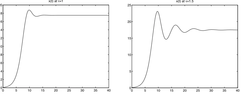
whererand K have the same meaning as the logistic equation (4.1) andτ > 0 is a constant. This equation is referred to as Hutchinson’s equation or the delayed logistic equation. This is a delayed differential equation which is an infinite dimensional equation which is properly posed in a function space requiring an initial function on −τ ≤t≤0 to generate a forward solution [24]. Several solutions are depicted in Figure 3.
0 5 10 15 20 25 30 35 40
0 2 4 6 8 10 12 14 16 18 20
x(t) at =1
0 5 10 15 20 25 30 35 40
0 5 10 15 20 25
x(t) at =1.5
Figure 3: Solution functions of the Hutchinson equation with a small delay τ = 1 (left) and a moderate delay τ = 1.5. The initial condition z0 = (x0, x(θ)) = (0.1,0.1) and parameter
values are r= 0.7 and K = 17.5.
There are several options for a “state space” to develop theoretical foundations for exis-tence, uniqueness, differentiability with repect to parameters, etc. One obvious choice [44] for an n-dimensional vector delay differential equation is C(−τ,0;Rn), however, the more common choice for computational efforts is a state space that treat the current state in a Eu-clidean sense while treating the history part in anL2 sense. That is,Z =Rn×L2(−τ,0;Rn),
sense. Note that the initial function need not be continuous at t = 0, and even if it is left continuous at t = 0, the solution itself need not be continuously differentiable, let alone analytic at t = 0. Moreover, non-analyticity in initial data can be propagated in solutions in time.
The sensitivity equations are derived in similar fashion as in the previous example and have the form (in general the sensitivity equations are also DDEs)
dx(t)
dt =rx(t)(1−
x(t−τ)
K ) (4.4)
dsr(t)
dt =r
1− x(t−τ)
K
sr(t)−rx(t)
K sr(t−τ) +x(t)
1− x(t−τ)
K
(4.5)
dsK(t)
dt =r
1− x(t−τ)
K
sK(t)−rx(t)
K sK(t−τ) +x(t)
x(t−τ)
K2
(4.6)
dsx0(t)
dt =r
1− x(t−τ)
K
sx0(t)−r
x(t)
K sr(t−τ) (4.7)
dsτ(t)
dt =r
1− x(t−τ)
K
sτ(t)−rx(t)
K [sτ(t−τ)−x˙(t−τ)] (4.8)
with initial conditions
x(θ) =x0, sr(θ) =sK(θ) = 0,−τ ≤θ≤0, sx0(0) = 1.
0 5 10 15 20 25 30 35 40 −20
−10 0 10 20 30 40 50 60
time t
xr(t)
complex−step sensitivity equations
0 5 10 15 20 25 30 35 40
−20 −10 0 10 20 30 40 50 60
time t xr(t)
complex−step sensitivity equations
0 5 10 15 20 25 30 35 40
0 2 4 6 8 10 12 14 16 18 20
time t
xK(t)
complex−step
sensitivity equations
0 5 10 15 20 25 30 35 40
0 2 4 6 8 10 12 14 16 18 20
time t xK(t)
complex−step sensitivity equations
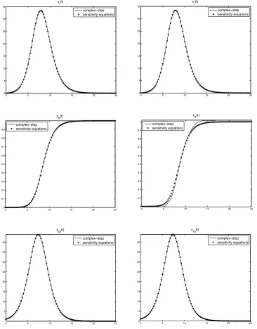
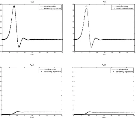
Figure 4: Comparison of sensitivity functions for the Hutchinson equation with respect to growth rate r, and carrying capacity K, each evaluated at (r, K, x0, τ) = (0.7,17.5,0.1,1).
The step size for the complex-step approximation is taken to be h = 10−40 (left) and h =
0 5 10 15 20 25 30 35 40 −20
−10 0 10 20 30 40 50 60 70 80
time t xx0(t)
complex−step sensitivity equations
0 5 10 15 20 25 30 35 40
−20 −10 0 10 20 30 40 50 60 70 80
time t xx0(t)
complex−step sensitivity equations
0 5 10 15 20 25 30 35 40
−5 0 5 10 15 20
time t x (t)
complex−step sensitivity equations
0 5 10 15 20 25 30 35 40
−5 0 5 10 15 20
time t x (t)
complex−step sensitivity equations
Figure 5: Comparison of sensitivity functions for the Hutchinson equation with respect to constant initial state x(θ) =x0 −τ ≤ θ ≤0, and delay τ, each evaluated at (r, K, x0, τ) =
4.3
Harmonic oscillator with delayed damping
As a third example we present the Minorsky harmonic oscillator with a delayed damping. This example arises in many physical applications where oscillatory phenomena are impor-tant and delayed damping is relevant. The equation has the form
d2x(t)
dt2 +K
dx(t−τ)
dt +bx(t) = g(t) (4.9)
where K and b are spring and damping constants. We use the complex-step method and sensitivity equations to determine regions of sensitivity for model parameters K, b and the time delayτ. To derive the sensitivity equations, we take the derivative of the equation with respect to each parameter. First let x1 =x(t) andx2 = ˙x(t) and rewrite equation (4.9) as a
first order system
dx1(t)
dt =x1(t) (4.10)
dx2(t)
dt =g(t)−bx1(t)−Kx2(t−τ). (4.11)
Letting s1(t) = ∂x∂K1(t), s2(t) = ∂x∂b1(t), s3(t) = ∂x∂τ1(t), s4(t) = ∂x∂K2(t), s5(t) = ∂x∂b2(t) and
s6(t) = ∂x∂τ2(t), the sensitivity equations are given by
ds1(t)
dt =s4(t), (4.12)
ds2(t)
dt =s5(t), (4.13)
ds3(t)
dt =s6(t), (4.14)
ds4(t)
dt =−bs1(t)−Ks4(t−τ)−x2(t−τ), (4.15) ds5(t)
dt =−bs3(t)−Ks6(t−τ) +Kx˙2(t−τ), (4.16)
with initial conditionsx(θ) =x0, −τ ≤θ≤0, si(0) = 0, i= 1,2,3,5, si(θ) = 0, i= 4,6. In Figure 6 the solutions of the sensitivity equations are shown for parameter values
0 5 10 15 20 25 30 35 40 45 50 −500 −400 −300 −200 −100 0 100 200 300 400 500
xb(t)
complex−step sensitivity equations
0 5 10 15 20 25 30 35 40 45 50
−500 −400 −300 −200 −100 0 100 200 300 400 500 x b(t)
complex−step sensitivity equations
0 5 10 15 20 25 30 35 40 45 50
−500 −400 −300 −200 −100 0 100 200 300 400 500
xK(t)
complex−step sensitivity equations
0 5 10 15 20 25 30 35 40 45 50
−500 −400 −300 −200 −100 0 100 200 300 400 500 x K(t) complex−step sensitivity equations
0 5 10 15 20 25 30 35 40 45 50
−500 −400 −300 −200 −100 0 100 200 300 400 500 x τ(t)
complex−step sensitivity equations
0 5 10 15 20 25 30 35 40 45 50
−500 −400 −300 −200 −100 0 100 200 300 400 500 x τ(t)
complex−step sensitivity equations
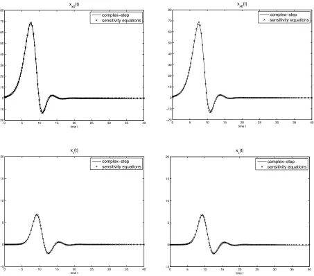
Figure 6: Comparison of sensitivity functions for the harmonic oscillator with delayed damp-ing with respect to the restordamp-ing rate b, damping coefficient K, and delayτ, each evaluated at (b, K, x0, τ) = (2,0.5,0.1,1). The step size for the complex-step approximation is taken
to beh= 10−40 (left) andh
4.4
Time delayed differential equations with non-smooth history
functions
In this section we test the complex-step method for DDEs with nonC1history function. Such systems arise in a wide class of applications, for example, when one has a discontinuous initial function such as x(θ) = 0 for −τ ≤ θ <0, x(0) =x0 6= 0 [24]. We note that discontinuities
in the history propagate to the solution in such a way that there is a jump in subsequent higher derivatives.
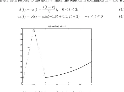
1. The first example is the Hutchinson equation (see Example 4.2) with a history function that has a jump in its first derivative at one point. We are interested primarily in the sensitivity with respect to the delay τ, since the solution is continuous inr and K.
˙
x(t) = rx(1−x(t−τ)
K ), 0≤t≤2τ (4.17)
x0(t) = φ(t) = min(−1.8t+ 0.1,2t+ 2), −τ ≤t≤0 (4.18)
−1 −0.5 0 0.5 1 1.5 2
0 0.1 0.2 0.3 0.4 0.5 0.6 0.7 0.8 0.9 1
φ(t) and x(t) at τ=1
φ(t)
x(t)
Figure 7: History and solution functions
Letsτ = ∂x∂τ(t), the sensitivity equation with respect to the delay is given by
dsτ(t)
dt =r
1− x(t−τ)
K
sτ(t)−r
x(t)
K [sτ(t−τ)−x˙(t−τ)] (4.19)
sτ(θ) = 0, −τ ≤θ ≤0 (4.20)
where
˙
x(t−τ) =
2 0≤t ≤τ /2
0 0.2 0.4 0.6 0.8 1 1.2 1.4 1.6 1.8 2 0
1 2 3 4 5 6x 10
−3 xτ(t)
complex−step sensitivity equations
0 0.2 0.4 0.6 0.8 1 1.2 1.4 1.6 1.8 2 0
1 2 3 4 5 6x 10
−3 xτ(t)
complex−step sensitivity equations
Figure 8: Complex-step approximation of ∂x∂τ overlaid with solution of the sensitivity equa-tions for Hutchinson’s equaequa-tions for t∈[0,2τ], τ = 1. The step size for the complex-step is taken to be 10−40 (left), h
crit= 10−320 (right, where h is taken too small). 2. Next we compute ∂x∂τ for the DDE:
dx
dt =x(t−τ), (4.22)
x0(t) =φ(t) = min{2t+ 2,−2t}, −1≤t ≤0.
The analytic solution for this problem is given by
x(t;τ) =
(t−τ)2+ 2t−τ2 for 0≤t ≤τ /2,
−(t−τ)2+ (τ−1)2+ 1/2 for τ /2< t≤τ.
(4.23)
The sensitivity equation with respect to τ is given by
dsτ
∂t =−x˙(t−τ) +sτ(t−τ), t >0, (4.24)
sτ(θ) = 0, −τ ≤θ ≤0. (4.25)
where sτ = ∂x∂τ(t) and
˙
x(t−τ) =
2 for 0≤t≤τ /2,
−2 for τ /2< t≤τ.
(4.26)
Recall the complex-step formula (2.5) is derived using the fact that the functionf is analytic. Once again these examples demonstrate that the complex-step method provides accurate approximation of the sensitivities when higher derivatives may have discontinuities. From this and other examples it is very clear that analyticity of the solution functions is sufficient
−1 −0.8 −0.6 −0.4 −0.2 0 0.2 0.4 0.6 0.8 1 0
0.1 0.2 0.3 0.4 0.5 0.6 0.7 0.8 0.9 1
φ(t) and x(t) at τ=1
φ(x)
x(t)
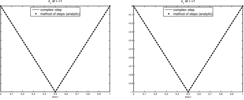
Figure 9: History and solution functions of equation (4.22) atτ = 1.
0 0.1 0.2 0.3 0.4 0.5 0.6 0.7 0.8 0.9 1 −1
−0.9 −0.8 −0.7 −0.6 −0.5 −0.4 −0.3 −0.2 −0.1 0
time t
x τ at τ =1
complex−step method of steps (analytic)
0 0.1 0.2 0.3 0.4 0.5 0.6 0.7 0.8 0.9 1 −1
−0.9 −0.8 −0.7 −0.6 −0.5 −0.4 −0.3 −0.2 −0.1 0
time t x
τ at τ =1
complex−step method of steps (analytic)
4.5
Elasticity Equations
As a final example, we compute the sensitivities of the solution u of the linear elasticity model with respect to the parameters µ, λ and a constant boundary condition g. Given a domain Ω⊂R2 with boundary∂Ω = Γ
0∪Γ1, the linear elasticity equations are given by the
system of PDEs:
−div(σu) = f, in Ω (4.27)
u= 0, on Γ0 (4.28)
σ(u)·¯n=g, on Γ1 (4.29)
Here the stress tensor σ(u) is given in terms of the strain (u) by the constitutive law:
σ(u) = λTr((u))I + 2µ(u),
where (u) = 12(Du+ (Du)T), and λ and µ are the Lam´e parameters.
In the following, we look at the cases when we have mixed Dirichlet-Neumann boundary and pure Dirichlet boundary conditions. We have documented a detailed explanation of the finite element method implementation for solving the linear elasticity equations in [16]. To compute the sensitivities using the complex-step method, we only add the increment ih to the desired sensitivity variable into the existing finite element program that solves (4.27), that is, we solve for u(λ +ih), u(µ+ih) and u(gk + ihk) and compute ∂u∂λi , ∂u∂µi , ∂u∂gki, respectively using equation (2.5). The sensitivity equations to compute sensitivities with respect to parametersµ and λ (Refer to [16] for derivation) are given by
−div(σ(u)) =f, in Ω
−div(σ(s1))− ∇(divu) = ∂f∂λ in Ω
−div(σ(s2))−∆u− ∇(divu) = ∂f∂µ in Ω
σ(u)¯n=g, on Γ1
(σ(s1) + (Tr(ε(u)))I)¯n= ∂g∂λ on Γ1
(σ(s2) + 2ε(u))¯n = ∂µ∂g on Γ1
u= 0, s1 = 0, s2 = 0 on Γ0
(4.30)
and the system for the sensitivity with respect to the boundary g reads:
−div(σu) =f, in Ω
−div(σr1) = 0, in Ω
−div(σr2) = 0, in Ω
u= 0, on Γ0
r1 = 0, on Γ0
r2 = 0, on Γ0
σ(u)·n¯ =g, on Γ1
σ(r1)·n¯ = (1,0), on Γ1
σ(r2)·n¯ = (0,1), on Γ1,
where s1 = ∂u∂λ , s2 = ∂µ∂u, r1 = ∂g∂u
1, and r2 =
∂u ∂g2.
The above system is solved using the finite element method (see [16] for details). In all of our computations, we use P-2 finite elements for spatial discretization, i.e., the solutionu
is approximated using polynomials of degree two. The mesh step size for the finite element discretization is taken to be k = 1/30.
As shown below in the figures, the complex-step approximations consistently agree with the ones obtained by deriving sensitivity equations up to some step size hcrit, where the complex-method starts to break down due to numerical underflow.
4.5.1 Elasticity system with mixed Neumann-Dirichlet boundary condition
In this first case, we consider the mixed Neumann-Dirichlet boundary problem. We take the domain Ω to be the unit square [0,1]× [0,1] with boundary ∂Ω = Γ0 ∪ Γ1 where
Γ0 = [0,1]× {0}and Γ1 =∂Ω\Γ0.
1. Sensitivities with respect to lam´e coefficients
We compute the sensitivities with respect to the coefficients µ and λ for the elasticity system at µ=λ= 1 with the right hand side and boundary data:
f =
2µy+ 4(µ+λ)xy−2(2µ+λ) 2µy2+ 2(2µ+λ)x2−2µx−3µ−λ
g =
µ(x2−y2+ 2xy2−3x+ 1)
2(2µ+λ)x2y−4µxy−λ(2x+y−1)
0
0.5
1
0 0.5
1 −0.4 −0.3 −0.2 −0.1 0
u1
−0.25 −0.2 −0.15 −0.1 −0.05 0
0
0.5
1
0 0.5
1 −0.25 −0.2 −0.15 −0.1 −0.05 0
u2
−0.2 −0.15 −0.1 −0.05
In Figures 12 and 13 we present a side by side comparison of the approximation of the sensitivity functions du1
dλ, du2 dλ, du1 dµ and du2
dµ computed using the complex-step and sensitivity equations methods.
0 0.5 1 0 0.5 1 −0.1 −0.05 0 0.05 0.1
du1/d
−0.06 −0.04 −0.02 0 0.02 0.04 0.06 0 0.5 1 0 0.5 1 −0.1 −0.05 0 0.05 0.1
du1/d
−0.06 −0.04 −0.02 0 0.02 0.04 0.06 0 0.5 1 0 0.5 1 −0.1 −0.05 0 0.05 0.1
du2/d
−0.08 −0.06 −0.04 −0.02 0 0.02 0.04 0 0.5 1 0 0.5 1 −0.1 −0.05 0 0.05 0.1
du2/d
−0.08 −0.06 −0.04 −0.02 0 0.02 0.04
Figure 12: Sensitivities of the solution u = (u1, u2) with respect to λ at λ = 1 computed
0
0.5
1
0 0.5
1 −0.1 −0.05 0 0.05 0.1
du1/dµ
−0.06 −0.04 −0.02 0 0.02 0.04 0.06
0
0.5
1
0 0.5
1 −0.1 −0.05 0 0.05 0.1
du1/dµ
−0.06 −0.04 −0.02 0 0.02 0.04 0.06
0
0.5
1
0 0.5
1
−0.1
−0.05 0 0.05 0.1
du2/dµ
−0.04
−0.02 0 0.02 0.04 0.06 0.08
0
0.5
1
0 0.5
1
−0.1
−0.05 0 0.05 0.1
du2/dµ
−0.04
−0.02 0 0.02 0.04 0.06 0.08
Figure 13: Sensitivities of the solution u = (u1, u2) with respect to µ at µ = 1 computed
The sensitivity function approximation with the complex-step method starts to decline after the critical step hcrit= 10−318 and it becomes meaningless for smaller values of h than that as seen in Figure 14.
0 0.5 1 0 0.5 1 −0.02 0 0.02 0.04 0.06 0.08 0.1
du1/d
0 0.01 0.02 0.03 0.04 0.05 0.06 0.07 0.08 0 0.5 1 0 0.5 1 −0.05 0 0.05 0.1 0.15 0.2
du2/d
−0.04 −0.02 0 0.02 0.04 0.06 0.08 0.1 0.12 0.14 0.16 0 0.5 1 0 0.5 1 −0.2 −0.1 0 0.1 0.2 0.3
du1/dµ
−0.1 −0.05 0 0.05 0.1 0.15 0.2 0.25 0 0.5 1 0 0.5 1 0 0.1 0.2 0.3 0.4
du2/dµ
0 0.05 0.1 0.15 0.2 0.25 0.3 0.35
Figure 14: Inaccurate approximations of the sensitivities by the complex-step method at
2. Sensitivity with respect to a constant boundary function
We compute the sensitivity of the solution to the elasticity system with respect to a constant boundary function g with the right hand side data:
f =
2µy+ 4(µ+λ)xy−2(2µ+λ) 2µy2+ 2(2µ+λ)x2−2µx−3µ−λ
g = (g1, g2) = (1,1).
0
0.5
1
0 0.5
1 −0.15 −0.1 −0.05 0 0.05 0.1
u1
−0.12 −0.1 −0.08 −0.06 −0.04 −0.02 0 0.02 0.04 0.06
0
0.5
1
0 0.5
1 −0.15 −0.1 −0.05 0 0.05 0.1
u2
−0.12 −0.1 −0.08 −0.06 −0.04 −0.02 0 0.02 0.04 0.06
0
0.5
1
0 0.5
1
−0.1 0 0.1 0.2 0.3
du1/dg1
0 0.05 0.1 0.15 0.2
0
0.5
1
0 0.5
1 −0.1 0 0.1 0.2 0.3
du1/dg1
0 0.05 0.1 0.15 0.2
0
0.5
1
0 0.5
1 −0.03 −0.02 −0.01 0 0.01 0.02 0.03
du2/dg1
−0.02 −0.015 −0.01 −0.005 0 0.005 0.01 0.015 0.02
0
0.5
1
0 0.5
1 −0.03 −0.02 −0.01 0 0.01 0.02 0.03
du2/dg1
−0.02 −0.015 −0.01 −0.005 0 0.005 0.01 0.015 0.02
Figure 16: Sensitivity of the solution u = (u1, u2) with respect to a constant boundary
functiong1 forg = (1,1) computed using the complex-step method (left) and the method of
0
0.5
1
0 0.5
1 −0.05 0 0.05
du1/dg2
−0.04 −0.03 −0.02 −0.01 0 0.01 0.02 0.03 0.04
0
0.5
1
0 0.5
1
−0.05 0 0.05
du1/dg2
−0.04
−0.03
−0.02
−0.01 0 0.01 0.02 0.03 0.04
0
0.5
1
0 0.5
1 0 0.05 0.1 0.15 0.2 0.25
du2/dg2
0 0.05 0.1 0.15 0.2
0
0.5
1
0 0.5
10 0.05 0.1 0.15 0.2 0.25
du2/dg2
0 0.05 0.1 0.15 0.2
Figure 17: Sensitivity of the solution u = (u1, u2) with respect to a constant boundary
functiong2 forg = (1,1) computed using the complex-step method (left) and the method of
4.5.2 Elasticity system with homogeneous Dirichlet boundary condition
In this example, we solve the elasticity system with homogeneous Dirichlet boundary condi-tion. Again we take Ω to be the square domain [0,1]×[0,1] with boundary ∂Ω = Γ0. The
right had data for the system is given by:
f =
−2(λ+ 2µ)(y2−y)−(λ+µ)(2x−1)(3y2−2y)−2µ(x2−x)
−2(λ+ 2µ)(x2−x)(3y−1)−(λ+µ)(2x−1)(2y−1)−2µ(y3−y2)
0
0.5
1
0 0.5
1 0 0.02 0.04 0.06 0.08
u1
0 0.01 0.02 0.03 0.04 0.05 0.06
0
0.5
1
0 0.5
10 0.01 0.02 0.03 0.04
u2
0 0.005 0.01 0.015 0.02 0.025 0.03 0.035
0 0.5 1 0 0.5 1 −1 0 1 2
x 10−8
du1/d
−4 −3 −2 −1 0 1 2 3 4 x 10⁻⁸
0 0.5 1 0 0.5 1 −2 −1 0 1 2 3
x 10−8
du1/d
−4 −3 −2 −1 0 1 2 3 4 x 10⁻⁸
0 0.5 1 0 0.5 1 −4 −2 0 2 4
x 10−8
du2/d
−3 −2 −1 0 1 2 3 4 5 x 10⁻⁸
0 0.5 1 0 0.5 1 −4 −2 0 2 4
x 10−8
du 2/d −3 −2 −1 0 1 2 3 4 5 x 10⁻⁸
Figure 19: Sensitivities of the solution u = (u1, u2) with respect to λ at λ = 1 computed
0 0.5 1 0 0.5 1 −2 −1 0 1
x 10−8
du1/dµ
−4 −3 −2 −1 0 1 2 3 4 x 10⁻⁸
0 0.5 1 0 0.5 1 −3 −2 −1 0 1 2
x 10−8
du1/dµ
−4 −3 −2 −1 0 1 2 3 4 x 10⁻⁸
0 0.5 1 0 0.5 1 −2 0 2 4 6
x 10−8
du2/dµ
−5 −4 −3 −2 −1 0 1 2 3 x 10⁻⁸
0 0.5 1 0 0.5 1 −2 0 2 4 6
x 10−8
du2/dµ
−5 −4 −3 −2 −1 0 1 2 3 x 10⁻⁸
Figure 20: Sensitivities of the solution u = (u1, u2) with respect to µ at µ = 1 computed
The sensitivity function approximation with the complex-step method starts to decline after the critical step hcrit = 10−314 and it becomes meaningless for smaller values ofh than that as seen in the figures below.
0 0.5 1 0 0.5 1 −4 −3 −2 −1 0
x 10−7
du1/d
−4.5 −4 −3.5 −3 −2.5 −2 −1.5 −1 −0.5 0 x 10−7
0 0.5 1 0 0.5 1 −2 −1 0 1 2
x 10−7
du2/d
−1.5 −1 −0.5 0 0.5 1 1.5 2 x 10⁻⁷
0 0.5 1 0 0.5 1 −2.5 −2 −1.5 −1 −0.5 0
x 10−7
du 1/dµ
−2.5 −2 −1.5 −1 −0.5 0 0.5 x 10⁻⁷
0 0.5 1 0 0.5 1 −1 0 1 2 3
x 10−7
du2/dµ
−0.5 0 0.5 1 1.5 2 2.5 x 10⁻⁷
For all of our computations, we used Matlab version 2014a on a Red Hat Linux Work-station featuring Intel(R) Core(TM) i7-2600 CPU - 3.40 GHz. For solving the DDEs, we modified the Matlab solver dde23 [63] to work for complex variables. For solving the elastic-ity equations in the last example, the complex-step is built into a finite-element solver. In the Table 1, we report on computation time for the examples presented.
Example No. Complex-Step Sensitivity Equations
4.1 0.29s 0.06s
4.2 0.43s 0.15s
4.3 7.59s 0.35s
4.4 (no.1) 0.04s 0.05s
4.4 (no.2) 0.03s 0.11s
4.5.1 (no.1) 5.21s 5.49s
4.5.1 (no.2) 2.92s 3.00s
4.5.2 4.81s 4.39s
Table 1: Computation times for the complex-step method and sensitivity equations in sec-onds.
5
Conclusions
We have demonstrated use of the complex-step method for computing sensitivities. The method is applied to examples of various complexity and the results are compared with solutions of traditional sensitivity equations. Even though there is a step size parameter
h to be chosen, the method gives consistently second order accurate approximation of the derivative starting from h as large as 10−2 up to h = hcrit which is on the order of 10−300 (approximately our machine precision ath= 10−324) with a true second order accuracy. Even
though the complex-step formula is derived assuming analyticity of the sensitivity function, we observed that the approximation provides accurate one-sided derivatives for functions with far less smoothness. Thus our conclusion is that analyticity of the solution functions is
sufficient but NOT necessary for the complex-step method to be effective.
One disadvantage of the complex-step approximation is when the number of sensitivity parameters to be considered is very large. In this case the method becomes computationally inefficient because to compute sensitivity with respect to each parameter, the increment
ih has to be added separately to the parameter of interest while the rest are kept constant. Therefore, the program needs to be run as many times as the number of the parameters being investigated. On the other hand the sensitivity equations give the sensitivities with respect to all the parameters at once as a vector, which can provide a big savings in computational times (see Table 1 for comparison of computation times). The complex-step approximation is still more robust when the dimension of the underlying dynamics is large compared to the number of parameters, this could be a big advantage. Even with this additional computational cost for problems with many parameters, its ease of implementation makes it a very good alternative to methods using the sensitivity equations. In light of the amount of effort involved in deriving sensitivity equations for complicated dynamical problems, the complex-step method could be a reasonable choice. Some of the pros and cons of the complex-complex-step method are summarized below:
Pros
• Easy to implement, no derivation of sensitivity equations required.
• The complexity of the algorithm is the same as the complexity of the algorithm eval-uating the function f (In our case, the algorithm solving the differential equations).
• Less computation time is needed if the number of parameters is not large compared to the dimension of the problem.
Cons
• A step size parameter is required.
For a problem of dimension n and m parameters, comparison of the complex-step ap-proximation with the use of sensitivity equations is summarized below.
Complex-Step Sensitivity Equations
Add a perturbation on existing algorithm New program to solve new set of equations.
Equations of size n to solve n+nm equations to solve
Has step size No step size
Need to run the programm times for each parameter
Program runs only once
Table 2: Comparison of the complex-step method and method of sensitivity equations.
Acknowledgments
This research was supported in part by the Air Force Office of Scientific Research under grant number AFOSR FA9550-12-1-0188 and and grant number AFOSR FA9550-15-1-0298.
References
[1] W. Kyle Anderson and Eric J. Nielsen, Sensitivity analysis for navier– stokes equations on unstructured meshes using complex variables, AIAA Journal, 39 (2001).
[2] W. Kyle Anderson, Eric J. Nielsen, and D.L. Whitfield, Multidisciplinary sensitivity derivatives using complex variables, Technical report, Engineering Research Center Re-port, Missisipi State University, mSSU-COE-ERC-98-08, July, 1998.
[3] J. Arino, L. Wang and G. Wolkowicz, An alternative formulation for a delayed logistic equation, J. Theo. Bio., 241 (2006), 109–118.
[4] H.T. Banks, Delay systems in biological models: approximation techniques, Nonlinear
Systems and Applications(V. Lakshmikantham, ed.), Academic Press, New York, 1977,
21–38.
[5] H.T. Banks, J.E. Banks, J. Rosenheim, and K. Tillman, Modeling populations ofLygus
Hesperus on cotton fields in the San Joaquin Valley of California: The importance
of statistical and mathematical model choice, CRSC-TR15-04, Center for Research in Scientific Computation, N. C. State University, Raleigh, NC, May, 2015; J. Biological
Dynamics, to appear.
[7] H.T. Banks and D. M. Bortz, A parameter sensitivity methodology in the context of HIV delay equation models, J. Math. Biol.,50 (2005), 607–625.
[8] H. T. Banks, D. M. Bortz and S. E. Holte, Incorporation of variability into the math-ematical modeling of viral delays in HIV infection dynamics, Math. Biosciences, 183
(2003), 63–91.
[9] H.T. Banks, A. Cintron-Arias, A. Capaldi and A. L. Lloyd, A sensitivity matrix based methodology for inverse problem formulation, CRSC-TR09-09, April, 2009; J. Inverse
and Ill-posed Problems, 17 (2009), 545–564.
[10] H.T. Banks, J. Catenacci and S. Hu, Asymptotic properties of probability measure esti-mators in a nonparametric model, SIAM/ASA Journal on Uncertainty Quantification, to appear.
[11] H.T. Banks, A. Cintron-Arias and F. Kappel, Parameter selection methods in inverse problem formulation, CRSC-TR10-03, N.C. State University, February, 2010, Revised, November, 2010; in Mathematical Modeling and Validation in Physiology: Application
to the Cardiovascular and Respiratory Systems,(J. J. Batzel, M. Bachar, and F. Kappel,
eds.), pp. 43 - 73, Lecture Notes in Mathematics Vol. 2064, Springer-Verlag, Berlin 2013.
[12] H.T. Banks, Marie Doumic, Carola Kruse, Stephanie Prigent, and Human Rezaei, In-formation content in data sets for a nucleated-polymerization model, CRSC-TR14-15, N. C. State University, Raleigh, NC, November, 2014; J. Biological Dynamics, (2015), DOI:10.1080/17513758.2015.1050465
[13] H.T. Banks, S. Hu, and W.C. Thompson, Modeling and Inverse Problems in the
Pres-ence of Uncertainty, Chapman & Hall/CRC Press, Boca Raton, FL, 2014.
[14] H.T. Banks, J.E. Banks, K. Link, J.A. Rosenheim, C. Ross, and K.A. Tillman, Model comparison tests to determine data information content, CRSC-TR14-13, N.C. State University, Raleigh, NC; Applied Mathematical Letters, 43 (2015), 10–18.
[15] J.E. Banks, H.T. Banks, K. Rinnovatore, C.M. Jackson, Optimal sampling frequency and timing of threatened tropical bird populations: a Modeling approach, Ecological
Modeling,303 (2014),70–77.
[16] H.T. Banks, K. Bekele-Maxwell, L. Bociu, M. Noorman and K. Tillman, Sensitivity analysis for elasticity equations. In preparation.
[17] H.T. Banks, Stacey L. Ernstberger and Sarah L. Grove, Standard errors and confi-dence intervals in inverse problems: Sensitivity and associated pitfalls , CRSC-TR06-10, March, 2006; J. Inverse and Ill-posed Problems, 15 (2007), 1–18.
[19] H.T. Banks, S. Dediu and H.K. Nguyen, Sensitivity of dynamical systems to parameters in a convex subset of a topological vector space , CRSC-TR06-25, September, 2006;
Math. Biosci. and Engr., 4 (2007), 403–430.
[20] H.T. Banks, S.L. Ernstberger and Shuhua Hu, Sensitivity equations for a size-structured population model, CRSC-TR07-18, September, 2007; Quarterly of Applied Mathemat-ics,LXVII (2009), 627–660.
[21] H.T. Banks and H.K. Nguyen, Sensitivity of dynamical systems to Banach space param-eters, CRSC-TR05-13, February, 2005; J. Math. Analysis and Applications,323(2006), 146–161.
[22] H.T. Banks and Keri L. Rehm, Experimental design for vector output systems, CRSC-TR12-11, N. C. State University, Raleigh, NC, April, 2012; Inverse Problems in Sci.
and Engr., 22 (2014) 557–590. doi:10.1080/17415977.2013.797973.
[23] H.T. Banks and K.L. Rehm, Parameter estimation in distributed systems: Optimal design, CRSC TR14-06, N. C. State University, Raleigh, NC, May, 2014; Eurasian
Journal of Mathematical and Computer Applications, 2 (2014), 70-79.
[24] H.T. Banks, Danielle Robbins and Karyn L. Sutton, Theoretical foundations for tra-ditional and generalized sensitivity functions for nonlinear delay differential equations CRSC-TR12-14, N. C. State University, Raleigh, NC, July, 2012; Math. Biosci. Engr.,
10 (2013), 1301–1333; http://dx.doi.org/10.3934/mbe.2013.10.1301
[25] H.T. Banks and H.T. Tran, Mathematical and Experimental Modeling of Physical and
Biological Processes, CRC Press, Boca Raton, FL, July, 2008, 308pp. published, January
2, 2009.
[26] L. Bociu, G. Guidoboni, R. Sacco, and J.T. Webster, Analysis of nonlinear poro-elastic and poro-visco-elastic models, Archive of Rational Mechanics and Analysis, 2015, sub-mitted.
[27] J.A. Burns, E.M. Cliff and S.E. Doughty, Sensitivity analysis and parameter estimation for a model of Chlamydia Trachomatis infection, J. Inverse Ill-Posed Problems, 15
(2007), 19–32.
[28] S.N. Busenberg and K.L. Cooke, eds., Differential Equations and Applications in
Ecol-ogy, Epidemics, and Population Problems, Academic Press, New York, 1981.
[29] V. Capasso, E. Grosso and S.L. Paveri-Fontana, eds., Mathematics in Biology and
Medicine, Lecture Notes in Biomath., Vol.57, Springer-Verlag, Berlin, Heidelberg, New
York, 1985.
[31] A. Casal and A. Somolinos, Forced oscillations for the sunflower equation, entrainment,
Nonlinear Analysis: Theory, Methods and Applications,6 (1982), 397–414.
[32] Paola Causin, Giovanna Guidoboni, Alon Harris, Daniele Prada, Riccardo Sacco, and Samuele Terragni, A poroelastic model for the perfusion of the lamina cribrosa in the optic nerve head, Mathematical Biosciences, (2014), March 11, submitted.
[33] J.M. Cushing,Integrodifferential Equations and Delay Models in Population Dynamics, Lec. Notes in Biomath., Vol. 20, Springer-Verlag, Berlin and New York, 1977.
[34] M. Davidian and D.M. Giltinan, Nonlinear Models for Repeated Measurement Data, Chapman and Hall, London, 2000.
[35] A. Ronald Gallant,Nonlinear Statistical Models, John Wiley and Sons, New York, 1987.
[36] U. Forys and A. Marciniak-Czochra, Logistic equations in tumor growth modelling,
Int.J. Appl. Math. Comput. Sci., 13 (2003), 317–325.
[37] Giovanna Guidoboni, Alon Harris, Lucia Carichino, Yoel Arieli and Brent A. Siesky, Ef-fect of intraocular pressure on the hemodynamics of the central retinal artery: A math-ematical model, Math. Biosci. Engr., 11 2014, 523–546. doi:10.3934/mbe.2014.11.523
[38] L. Glass and M. C. Mackey, Pathological conditions resulting from instabilities in phys-iological control systems, Ann. N. Y. Acad. Sci. 316 (1979), 214–235.
[39] B.C. Goodwin, Temporal Organization in Cells: a dynamic theory of cellular control
processes, Academic Press, London, 1963.
[40] B.C. Goodwin, Oscillatory behavior in enzymatic control processes,Adv. Enzyme Reg.,
3 (1965) 425–439.
[41] K. Gopalsamy, Stability and Oscillations in Delay Differential Equations of Population
Dynamics, Kluwer, Dordrecht, 1992.
[42] Rafael Grytz, G¨unther Meschke and Jost B. Jonas, The collagen fibril architecture in the lamina cribrosa and peripapillary sclera predicted by a computational remodeling approach,Biomech Model Mechanobiol.,10 (2011), 371—382 DOI 10.1007/s10237-010-0240-8.
[43] K. P. Hadeler, Delay equations in biology, in Functional differential equations and
ap-proximation of fixed points (H. O. Peitgen and H. O. Walther, eds.), Lect. Notes Math.
730 Springer-Verlag Berlin, 1979, 136–156.
[44] J. Hale, Theory of Functional Differential Equations, Springer-Verlag, New York, 1977.
[46] G. E. Hutchinson, Circular causal systems in ecology, Annals of the NY Academy of
Sciences,50 (1948), 221–246.
[47] G. E. Hutchinson, An Introduction to Population Ecology, Yale University, New Haven, 1978.
[48] Mark Kot,Elements of Mathematical Ecology, Cambridge University Press, Cambridge, 2001.
[49] Y. Kuang, Delay Differential Equations With Applications in Population Dynamics, Vol. 191 of Mathematics in Science and Engineering, Academic Press, New York, NY, 1993.
[50] Kok-Lam Lai, Generalizations of the complex-step derivative approximation, PhD the-sis, University at Buffalo, Buffalo, NY, 2006.
[51] J. N. Lyness, Numerical algorithms based on the theory of complex variables, Proc.
ACM 22nd Nat. Conf., 4 (1967), 124—134.
[52] J. N. Lyness and C. B. Moler, Numerical differation of analytic functions, SIAM J.
Numer. Anal., 4(1967), 202—210.
[53] N. MacDonald, Time lag in a model of a biochemical reaction sequence with end-product inhibition, J. Theor. Biol., 67 (1977), 727–734.
[54] N. MacDonald, Time Lags in Biological Models, Lecture Notes in Biomathematics 27, Springer, Berlin, 1978.
[55] Joaquim R. R. A. Martins, Ilan M. Kroo, and Juan J. Alonso. An automated method for sensitivity analysis using complex variables. AIAA Paper 2000-0689 (Jan.), 2000.
[56] Joaquim R. R. A. Martins, Peter Sturdza, and Juan J. Alonso. The complex-step deriva-tive approximation. Journal ACM Transactions on Mathematical Software (TOMS), 2003.
[57] N. Minorsky, Self-excited oscillations in dynamical systems possessing retarded actions,
Journal of Applied Mechanics, 9 (1942) A65–A71.
[58] N. Minorsky, On non-linear phenomenon of self-rolling, Proceedings of the National
Academy of Sciences, 31 (1945), 346–349.
[59] N. Minorsky, Nonlinear Oscillations, Van Nostrand, New York, 1962.
[60] S. I Rubinow, Introduction to Mathematical Biology,J. Wiley, New York, 1975.
[62] G.A.F. Seber and C.J. Wild, Nonlinear Regression, J. Wiley & Sons, Hoboken, NJ, 2003.
[63] Lawrence F. Shampine and Skip Thompson, Solving ddes in matlab,Applied Numerical
Mathematics, 37, No. 4 (2001), 441–458.
[64] F. R. Sharpe and A. J. Lotka, Contribution to the analysis of malaria epidemiology IV: Incubation lag, supplement to Amer. J. Hygiene 3 (1923), 96–112.
![Figure 8: Complex-step approximation of ∂x∂τ overlaid with solution of the sensitivity equa-tions for Hutchinson’s equations for t ∈ [0, 2τ], τ = 1](https://thumb-us.123doks.com/thumbv2/123dok_us/1750609.1224488/20.612.106.506.63.224/figure-complex-approximation-overlaid-solution-sensitivity-hutchinson-equations.webp)