The maintenance of single-locus polymorphism. I. Numerical studies of a viability selection model.

The Maintenance of Single-Locus Polymorphism.

I.

Numerical Studies

of

a Viability Selection Model

Hamish G.

Spencer,**t9’

and R.

William Marks*

*Department ofBiologica1 Sciences, Stanford University, Stanford, Calqornia 94305, tMuseum of Comparative Zoology, Haruard University, Cambridge, Massachusetts 02138, and $Department of Biology, Villanova University, Villanova, Pennsylvania 19085

Manuscript received October 5, 1987 Revised copy accepted July 1 , 1988

ABSTRACT

The ability of viability selection to maintain single-locus polymorphism is investigated with two models in which the population is bombarded with a series of mutations with random fitnesses. In the first model, the population is allowed to reach equilibrium before mutation resumes; in the second the iterations and mutation occur simultaneously. Monte Carlo simulations of these models show that viability selection is easily able to maintain stable 6- or 7-allele polymorphisms and that monomorphisms and diallelic polymorphisms are uncommon. The question of how monomorphisms arise is also discussed.

H

OW large amounts of genetic variation are pre- served in populations has been a recurring ques- tion in theoretical population genetics since the advent of electrophoresis in the late 1960s revealed that such variation was widespread [see LEWONTIN (1 974) for a discussion]. However, most of the theoretical models so far examined suggest that multiallele (one-locus) polymorphisms are extremely difficult to construct. LEWONTIN, GINZBURG and TULJAPURKAR (1 978)

showed that under constant viability selection the proportion of randomly generated fitness matrices that lead to stable, feasible polymorphisms for more than five alleles was vanishingly small (see also GIL-

LESPIE 1977). They also looked at the cases in which

the loci were pairwise heterotic (i.e., each heterozygote had greater viability than both the corresponding homozygotes) and totally heterotic (i.e., all heterozy- gotes were fitter than the fittest homozygote). Again they found that the chances of stable feasible poly- morphisms were miniscule.

In a study of structured fitness matrices, KARLIN

(198 1) showed that the probability of a (globally) stable equilibrium was greater than in the purely random case. For example, in the “generalized domi- nance fitness model” (in which the alleles have a dominance ordering A I

<

A2

< .

. .

<

Ar and the fitness

of A, A, is given by a, for i

<

j and that of A, A, by bj) the probability of a stable 5-allele polymorphism is about 0.0062, about 100 times the probability for a “random” matrix. When the aj and bj are ordered (ai

<

a, and bi

<

b, for all i

<

j ) then the probability increases t o about 0.1 113. This latter model also maintains a fairly large number of alleles at equilib-

’

Present address and address for correspondence: Department of Math- ematics and Statistics, University of Auckland, Private Bag. Auckland, New Zealand.

Genetics 1 4 0 605-613 (October, 1988)

rium (given a larger number in the initial frequency distribution) (KARLIN and FELDMAN 198 1). For ex- ample, when starting with eight alleles, the average number at equilibrium was 3.17 compared to 1.68 in the random case.

CLARK and FELDMAN (1986) found no qualitative difference between random single-locus fertility and random viability models in their ability to maintain large levels of polymorphism.

The theoretical population genetics problem of how alleles are maintained is analogous to the stability vs. complexity problem in theoretical ecology. The greater the number of species present in a community the smaller is the proportion of the ecological param- eter space that permits all the species to coexist (MAY

1974). One approach to the ecological problem has been to change the question from “Are stable multi- species communities rare in parameter space?” to “Are multispecies communities hard to construct?” (TAY- LOR 1985). TAYLOR has shown that by introducing species one at a time to an already stable multispecies community, the number of species present can be increased to quite high levels. Sometimes the intro- duction of the new species can trigger a partial collapse of the system, but over time the number of species will increase. Hence, although multispecies commu- nities are rare in the total parameter space, they may not be hard to reach.

The analogous approach has been used here to see if multiallele polymorphisms are hard to construct.

DYNAMICS OF VIABILITY SELECTION AND MUTATION

606 H. G. Spencer and R. W. Marks

greater than the mean fitness of the population at the equilibrium, i.e., w, + 1 ,

.

w, +

.

>

zlr (KINCMAN 196 1). If it does invade then the changes in allele frequencies will be governed by

p l

= wi ,

.

wi,

.

pi p;/G, for

i = 1, 2,

. .

.,

n

+

1 (1)

in which pi is the frequency of the ith allele at gener- ation t ,

p l

is the frequency at generation t

+

1,

w;,. = wit,

p,

is the marginal fitness of the ith allele at generation t ,

wij is the viability of an individual with genotype AiA, and

zlr =

x

w,,&p, is the mean fitness of the population at generation t .

An equilibrium is reached when

p i

=

pi

for all i = 1, 2,

. .

.,

n

+

1. For the one locus viability model KINCMAN (1 96 1) has shown that at most one (n

+

1)- allele polymorphism is stable for a given set of w;j values and that it is globally stable. Hence it will be reached irrespective of the value of the n-allele poly- morphism. Of course, the successful invasion of the (n

+

1)th allele may not result in a stable (n

+

1)-allele polymorphism, but instead in the extinction of one or more of the alleles present in the n-allele polymor- phism.

AOKI (1980) used this dynamic to see how often a stable n

+

1 allele polymorphism was reached after an unbroken run of n successful increasing invasions. (By an increasing invasion we mean an invasion leading from a stable n-allele polymorphism to a stable (n

+

1)-allele polymorphism. By contrast, a decreasing in- vasion leads to a decrease in the number of alleles present at the new equilibrium, while in a replacement invasion the invading allele drives one other to extinc- tion leaving the system with an n-allele polymor- phism.) AOKI looked at the stability of the new system in which the fitnesses of the mutant (i.e., the wi,, + 1’s i = 1, 2,

. .

.,

n

+

1) were drawn from the uniform distribution on ( 0 , 1). His results indicated that the most likely outcome was the repulsion of the invading allele, i.e., it did not successfully invade. T h e next most likely was a replacement or a decreasing invasion, and always the least likely was an increasing invasion. Moreover, the probability of an increasing invasion given that there was an invasion was a decreasing function of n. These results held for n = 2, 3, 4 and 5 and when the w , , ~ + 1’s were drawn from a

p

(3, 3) distribution. Furthermore, the probability of success- ful invasion decreased as the number of alleles in- creased, but this is confounded by the fact that zir

increases monotonically over time and the greater zir

the harder it is for a mutant to invade, everything else being equal (see below).

AOKI also conducted two runs in which he looked

at all systems, not just those with unbroken runs of increasing invasions. If the mutant invaded success- fully he iterated Equation 1 to equilibrium and found that some polymorphisms were remarkably stable to invasion, one run maintaining a seven-allele polymor- phism in the face of 94,266 mutations. T h e other run, however, was unable to sustain more than two alleles, although it ran for only 36 mutations.

MODEL 1-MUTATION W I T H INTERVENING EQUILIBRATION

This first model was very similar to AOKI’S latter model. The initial system consisted of one allele with w1,l = 0.5 and was bombarded with new mutants (potential second alleles), the w;,2 (i = 1 , 2 ) being drawn from the uniform distribution on ( 0 , 1). If the mar- ginal fitness of a new mutant was greater than the mean fitness, i.e., w2 ,

.

wp> zlr (w1,p

>

w l , 1) we had a successful invasion and Equation 1 was iterated to equilibrium. T h e invading allele was given an initial frequency of an allele was considered extinct if its frequency fell below 5 X and equilibrium was defined as the point at which the maximum change in allele frequency in one generation was less than 5 x This sequential invasion process was repeated until the required number of invasions had occurred. T h e simulations were written in Pascal, compiled with the TURBO-87 compiler and performed on an IBM- X T microcomputer. The (pseudo)random numbers came from a lagged Fibonacci generator (KNUTH

1981), as the TURBO generator does not correctly supply a uniform distribution.

MODEL 1-RESULTS

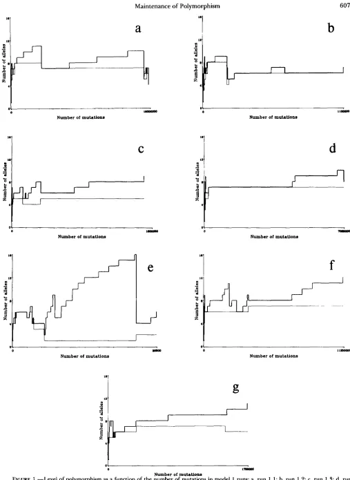
T h e levels of polymorphism for seven replicate runs (runs 1.1-1.7) are shown in Figure 1 and Table 1. Run 1.4 had 25 invasions, run 1.7 28 and the rest 40. Clearly the number of alleles maintained under this scheme is much larger than might be expected from a naive reading of LEWONTIN, GINZBURC and TULJA- PURKAR’S (1978) results. T h e minimum number of alleles after 1 O4 mutations (which was about the length of time until the system settled down) was 4, and it was not unusual to observe

7

or 8. This was also true if we restrict ourselves to “common” alleles, by which

we mean those with frequencies of 0.01 or greater. Many multiallele polymorphisms were resistant to invasion. T h e most resistant was run 1.4, in which a 7-allele polymorphism repulsed 4,2 10,363 mutants. T h e vulnerability of a polymorphism to invasion is a function of zir and the number and frequencies of

1..

a

I2

0

0 -1

Number of mutations

1.'

1x1

C

0 -1

Number of mutations

0

N u m b e r of mutations

I O

IZ

01

a

b

0 1 l a o m

Number of mutations

"1

d

121

0

-

Number of mutations

f

osm 0

Number of mutations

1 1 z 5 o o O O

I

TABLE 1

H. G. Spencer

Model 1-levels of polymorphism

No. of alleles Run attempts No. successful Total Common ui

No. invasion

1 . 1 15,814,342 40 5 4 0.9718

1.2 1,098,893 40 7 6 0.9672

1.3 1,506,796 40 9 5 0.9785

1.4 7,006,429 25 8 7 0.9703

1.5 20,446 40 6 2 0.9940

1.6 11,161,155 40 12 7 0.9704

1.7 1,742,571 28 11 6 0.9624

TABLE 2

Model 1-measures of evenness for three 7-allele polymorphisms

Run Theoretical mini-

Measure" mum/maximum 1.2 1.3 1.4

2 0.00000 0.02718 0.04178 0.02533

H 0.8571 0.6669 0.5647 0.6799

E 1.9459 1.3649 1.0500 1.3662

liJ 1

.oooo

0.96564 0.97851 0.96963

No. mutations 105,650 164,013 4,210,363

repulsed

2 = variance =

x(#;

-

# / n , where of course n = 7 and ji =

%; H = heterozygosity = 1

-

x p : ; E = entropy = -CpJnp;.

complex way: more even allelic distributions are more resistant to invasion. This is because more of the w,,, + matter in the calculation of w, +

,.

.

If, for example, allele

k

is rare, then it is irrelevant what wk,, + is-it contributes very little to wn +

,.

.

T h e success of the mutant thus depends on the w,,, + 1's in which allele i is common, and the fewer of these the greater the chance of success. This boils down to the probability that the weighted sum of n uniform ran- dom numbers on (0, 1) will exceed zir, a constant (%). In general the weighted sum has mean L/2 and variance

p?/12. For an absolutely even distribution the weights ( i . e . , the pi's) are all l / n and so the variance is 1/(12n). As n becomes larger, the distribution of the weighted sums becomes bell-shaped ($ the central limit theorem). At the other extreme, a very uneven distribution has n

-

1 of the pi's close to 0.0 and one

1.0, and so the variance is Y 1 2 , much larger than before. T h e larger the variance the greater the prob- ability that a particular sum will exceed the zir thresh- old. Thus the variance of the allele frequencies is the best measure of the invadability of a polymorphism. Increasing the number of alleles in a polymorphism often, but not always, increases the evenness of the allelic distribution and if it does so will also increase the polymorphism's stability to invasion. Various measures of evenness for three actual 7-alleles poly- morphisms are shown in Table 2. These all show that the more even the allelic distribution, the more resist-

and W. Marks

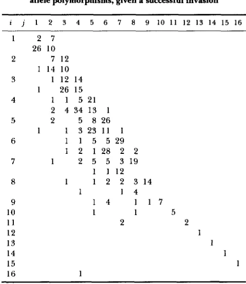
TABLE 3

Model 1-No. of transitions from i-allele polymorphisms to j -

allele polymorphisms, given a successful invasion

I j 1 2 3 4 5 6 7 8 9 1 0 1 1 1 2 1 3 1 4 1 5 1 6

1 2 7

26 10 2 7 12

1 14 10 3 1 12 14

1 26 15

4 1 1 5 2 1

2 4 34 13 1

5 2 5 8 2 6

1 1 3 23 11 1

6 1 1 5 5 2 9

1 2 1 2 8 2 2

7 1 2 5 5 3 1 9

8 1 1 2 2 3 1 4

9 1 1 7 1 4

1 1 12

1 1 4

10 1 1 5

1 1 2 2

12 1

13 1

14 1

15 1

16 1

The first (or only) line of numbers is the number of transitions between polymorphisms counting all alleles; the second counts only common ones. Blanks indicate zeros.

ant to invasions the polymorphism was, allowing for the differences in 6.

T h e numbers of transitions between levels of poly- morphism in runs 1.1-1.7 are shown in Table 3. T h e elements on the diagonal represent replacement in- vasions, those below it decreasing invasions and those above increasing invasions. Inspection of Table 3 and Figure 1 reveals that decreasing invasions often led to extinction of more than one allele. This was in part a consequence of a quasi-equilibrium being reached in which the frequencies of rare transient alleles change very slowly before extinction (which looks like a true equilibrium to the program) and hence some of the levels of polymorphism are inflated. T h e same pattern was observed, however, with the common alleles. Ta- ble 3 shows that for common alleles the transition from n to n

-

1 alleles occurred eleven times and that from n to n

-

2 or less, ten. This is not surprising given the nature of the equilibria: if the maintenance of an allele is thought of as being partitioned among the alleles, then because alleles mutually maintain each other, the extinction of one allele may easily remove the main support of another, driving the latter to extinction.

Run 1.5 (Figure 1 e) showed the most extreme quasi- equilibria. Only at the two major extinctions, when the number of alleles fell from 9 to 5 and 16 to 4,

Equation 1 and so the true levels of polymorphism were probably in the vicinity of 4 or 5 alleles for most of this history. Note that at the latter extinction the number of common alleles increased. An increase in the number of common alleles at the same time as a decrease in the total number of alleles as the system moved to a true equilibrium was not uncommon.

Run 1.5 also illustrates one reason that mono- morphism may be hard to reach. The early polymor- phism with three common alleles at 2991 to 4489 mutations had a mean fitness of 0.93859, while after the successful invasion that brought the system to monomorphism (with respect to common alleles) 13 was 0.99388. For an invasion leading to monomorph- ism to occur the new mutation must have most wi,, + 1 (i # n

+

1) less than wn + I,, + 1. Since w, + I , ~ + I is

irrelevant to the calculation of w, + 1,. and hence the success of the invasion itself, mutations with low w, + 1.

+ 1 values are not selected out, at least not until they are common. T h e method of generating the wi,, + 1's in the simulation may appear to exacerbate this fea- ture: because the maximum value of any wi,,, + 1 is 1 , the wLn + (i # n

+

1) of successful invaders will become closer and closer to 1 as the simulation pro- ceeds and yet the w , + l.n + 1 will continue to range

from 0 to 1 . However, drawing the wi,

,

+ 1 from an unbounded distribution (say a normal) may not make much difference because the w, + I,, + 1 are irrelevant to the success of the invasion and will often be less than most if not all the wi,, + I (i # n

+

1). Studies of

this modification to the model are underway. T h e distributions of the alleles during the runs showed a wide range of forms. Some polymorphisms had J-shaped distributions: one allele would be by far the commonest with the remainder less than lo%,

e.g., in run 1.2, the %allele polymorphism lasting from mutations 35524 to 93083 had one allele at a fre- quency of 0.7736, the others being at 0.0623, 0.0581, 0.0292,0.0262, 0.0261, 0.0125 and 0.0120. Later in the same run, the 6-allele polymorphism lasting from mutations 638,938 to 1,098,893 had a more even distribution, the frequencies being 0.4828, 0.1462, 0.1418, 0.1028, 0.0782 and 0.0483. T h e final equi- librium in run 1 . 1 showed no predominant allele- the frequencies here were 0.3539, 0.3403, 0.1614, 0.1443 and 0.0001.

T h e form of some of the wit, matrices was also investigated. Of the six matrices examined one showed total heterosis, four were pairwise heterotic, and one had a heterozygote less fit than one of its (two) corresponding homozygotes. In this last case the distribution was noticeably J-shaped, one allele ac- counting for 0.7749 of the frequency distribution. Its homozygote fitness was greater than 13 of the 21 heterozygote fitnesses (there were 7 alleles present at equilibrium), but not one of the 13 involved that

allele. T h e heterozygotic fitness (0.6318) that was lower than its corresponding homozygotic fitness (0.6693), involved one extremely rare allele (with homozygotic fitness 0.4001), so that the frequency of the heterozygote involved would have been 2pqwP,J

zz, =

5.7

x lo-*.

MODEL 2-MUTATION WITH SIMULTANEOUS EQUILIBRATION

Model 1 assumes that equilibrium will always be reached before a new mutant can invade the popula- tion. To see what effect this had on the results above and to get around the quasi-equilibrium problem, the model was altered so that new mutants arose while Equation 1 was still being iterated. T h e number of mutations occurs according to a Poisson distribution with mean m mutants per generation ( i e . , per itera- tion). Simulations were run for 1

o6

generations.

MODEL 2"RESULTS

a

O t

0 soom 6c4ono nmon IOOODDO

Number of ganerationa

C

0 amno 6mnoa noom OlOODDO

Number of generations

e

0 . . .

0 zomm Moo00 mow0 l O D o m 0

Number of generations

b

O L - . . . , . .

0 amno 6c4ono 11OOOO L O D O D D O

Number of generatioas

d

o l

0 amno asmoo noom IDODD0

Number of generations

f

0

0 zwoao smooo mow0 lDmm0

Number of generations

h

ol . . .

0 zomm smooo moo00 l D o o p m 0 zomm soom0 wmo lmoD00

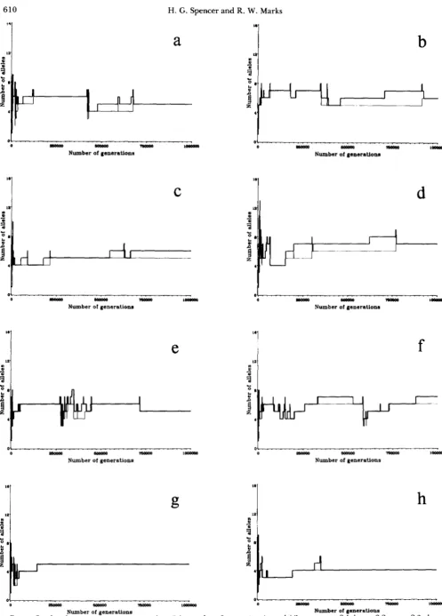
FIGURE 2.-Level Number ot polymorpnlsm as a runction of the number of generations in model 2 runs: a , run 2.1; b, run 2.2; c, run 2.3; d , run

of generations Number of generations

2.4; e , run 2.5; f, run 2.6; g, run 2.7; h , run 2 .8. Heavy (upper) lines indicate the total number of alleles, light (lower) lines indicate the number of common alleles.

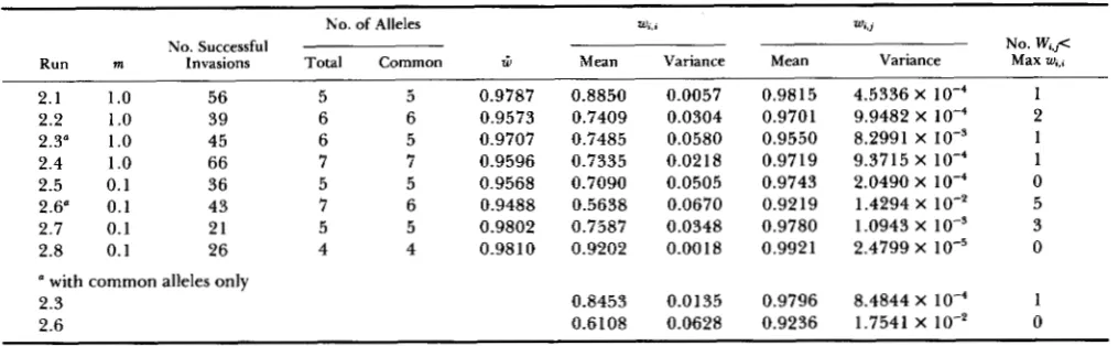
TABLE 4

Model 2-levels of polymorphism and statistics of fitnesses

No. of Alleles W.,. Wi,

No. Successful No. W,,,<

Run m Invasions Total Common i Mean Variance Mean Variance Max

2.1 1.0 56 5 5 0.9787 0.8850 0.0057 0.9815 4.5336 X loF4 1

2.2 1.0 39 6 6 0.9573 0.7409 0.0304 0.9701 9.9482 X 2

2.3“ 1.0 45 6 5 0.9707 0.7485 0.0580 0.9550 8.2991 X IO-’ 1

2.4 1.0 66 7 7 0.9596 0.7335 0.0218 0.9719 9.3715 X 1

2.5 0.1 36 5 5 0.9568 0.7090 0.0505 0.9743 2.0490 X 0

2.6” 0.1 43 7 6 0.9488 0.5638 0.0670 0.9219 1.4294 X lo-‘ 5

2.7 0.1 21 5 5 0.9802 0.7587 0.0348 0.9780 1.0943 X lo-’ 3

2.8 0.1 26 4 4 0.9810 0.9202 0.0018 0.9921 2.4799 X 0

Ii with common alleles only

2.3 0.8453 0.0135 0.9796 8.4844 X 1

2.6 0.6108 0.0628 0.9236 1.7541 X lo-’ 0

was 0.1 this was not nearly so apparent: the longer intervals between invasions allowed more equilibra- tion and extinction. Also, when the number of alleles had recently been reduced a rapid series of invasions could occur. This is because the system is effectively unchanged after a successful invasion and invasion can occur easily because the number of alleles is small. T h e difference in initial behavior between runs with different m values suggests that m is an important parameter in a system with few alleles. Suppose that

m was large enough so that several mutants invaded before equilibrium was reached. If these same muta- tions arose but at a different rate ( i e . , m was different), then the subsequent polymorphism could well be dif- ferent. This is because the success of a mutant may well depend on the w , , ~ + 1 of the ith allele (say) which would have been extinct or rare and hence irrelevant to the mutation’s success if the mutation had arisen later. Thus not only is the order of events important in evolution (see, e.g., LEWONTIN 1967), but so is the rate at which they occur.

T h e main difference between the results of models 1 and 2 is in the number of rare alleles present. As was noted above, the quasi-equilibrium problem of model 1 means that the levels of polymorphism for the total number of alleles is probably inflated. In model 2 this problem is removed and although the number of common alleles does not appear to be different, the number of rare alleles is not usually greater than one. When more than one rare allele is present, it is most frequently immediately after an invasion and the system is probably not at equilibrium.

T h e forms of the distributions of alleles were similar to those in model 1 , with some J-shaped (e.g., the end of run 2.7) and others very even (e.g., the end of run 2.4) and most in between. T h e final 8 wtd matrices showed two cases of total heterosis (runs 2.5 and 2.8) and 6 of pairwise heterosis. Note that the two runs that resulted in total heterosis had the two lowest

levels of polymorphism (5 and 4 alleles, respectively) and neither had any rare alleles. In contrast, the furthest departure from total heterosis, run 2.6, had 2 homozygotes fitter than 5 heterozygotes and an- other homozygote fitter than 3 (of the same) hetero- zygotes and maintained 7 alleles, 6 of which were common. A more detailed investigation of a much larger sample of such matrices may be found in MARKS and SPENCER ( 1 989).

T h e differences and similarities between runs with

m = 1 .O and those with m = 0.1 are interesting. There was no significant difference in ZZ, at either lo5 or l o6 generations (indeed at the latter the mean of the 13’s

was greater for m = O.l!). T h e number of successful invaders, however, was different ( t = 3.598, P

<

0.02 and t = 2.593, P

<

0.05 at lo5 and lo 6 generations respectively), those runs with m = 1.0 having about 2.05 (lo5 generations) and 1.65 ( lo6 generations), times the number of successful invasions as those with

m = 0.1.

DISCUSSION

T h e above models show that viability selection is capable of maintaining as many as eight alleles in a population. This is in spite of the fact that random fitness matrices leading to stable feasible equilibria with five of more alleles are extremely rare (LEWON-

TIN, GINZBURC and TULJAPURKAR 1978). Even when the matrices are given some nonrandom structure, the probability of stability is still low (KARLIN 1981 ;

612 H. G. Spencer and R. W. Marks

lose one or more alleles. Third, and most important, natural populations are more realistically thought of as being the results of a nonrandom selective process that weeds out unstable fitness matrices (and in partic- ular the more pathological alleles) and leaves popula- tions at stable polymorphisms. Furthermore, these stable polymorphisms are most unlikely to be the result of a series of monotonically increasing polymor- phisms of lesser degree, as in AOKI’S (1980) model. Rather, the periodic collapses of a polymorphism when a new mutant invades the population strengthen the resistance of the system to further invasions. It should be noted, however, that the models were una- ble to maintain an extremely large number of alleles, such as occurs at the esterase-5 locus in Drosophila pseudoobscura with at least 41 alleles (KEITH 1983).

T h e ability of viability selection to maintain poly- morphisms and the speed with which new mutants invade after a collapse raise the question of how monomorphisms and diallelic polymorphisms arise. One possible answer is that the population sizes are smaller than in the models. In model 2, m = 2Ncp, where N e is the effective population size and p the mutation rate. Hence reducing Ne is tantamount to decreasing m and this does result in a decrease in ne,

the effective number of alleles in the population: at the end of runs 2.1-2.4 (m = 1 .O) ne = 3.452, whereas at the end of runs 2.5-2.8 (m = 0.1) ne = 2.5061. A parallel argument holds for a reduction in the muta- tion rate p. Incorporation of a finite population size also introduces the effect of drift which would elimi- nate some of the rare alleles. This is unlikely, however, to alter either the number of common alleles or ne,

unless the population size is quite small (less than 1000). We are currently investigating the effects of drift on these models.

T h e distributions of model 2 can be compared with those of the neutral infinite allele model [see EWENS (1979) for a complete description]. T o see how close the distributions are we can ask what number of genes would need to be sampled from one of the final model 2 distributions in order to reject neutrality in favor of heterosis. We used a 5 % significance level and as- sumed that the sample homozygosities are the same as those of the distributions from which they are sampled. From the table in Appendix C of EWENS (1 979) we see that for all the distributions, except that of run 2.4, many more than 500 genes would need to be sampled. For run 2.7 it is unlikely that any sample size could distinguish the neutral and actual distribu- tions. In run 2.4 a sample of at least 200 would be required. Because the fitnesses were drawn from a range with a upper bound of 1 and zi, is nondecreasing, over time more and more of the alleles present in the population have w,,, values very close to 1. This means that, not only does the invadability of the polymor- phism decrease, but also the differences in heterozy-

gote fitnesses become smaller. T h e model is slow to converge to a neutral one, however, since the homo- zygote fitnesses increase at a much slower rate (MARKS and SPENCER 1989).

One shortcoming of the above models is that they assume constant fitnesses for an inordinately long time. These simulations, however, could have been started at any point in their history and the same results obtained. Indeed, this rationale enables us to ignore the first 1000 or so generations of model 2 runs if we consider the low initial zi, unrealistic. Never-

theless, random fluctuations or small but persistent decreases in the fitnesses might be expected to lead to different levels of polymorphism. We are currently investigating models of this type. Note, however, that the rapid increase in the number of alleles at the start of every run suggests that such models will not show long periods of reduced variability.

One interesting extension of the models would be to change the way the w ; , ~ + 1 are generated. It seems more probable that there would be some correlation between the values (including wn + l , n + and this might make invasion easier. It is not clear what effect this would have on the level of polymorphism, but AOKI’S (1 980) results suggest that it might reduce it slightly.

We have greatly benefited from discussions with K. AOKI, A. CLARK, M. FELDMAN, R. LEWONTIN, G. MAYER, S. TULJAPURKAR and M. TURELLI on this an related subjects and we thank them for their help. L. GINZBURG and two anonymous reviewers also pro- vided numerous useful suggestions. P. DANAHER and G. MARSACLIA kindly supplied us with the random number generator. This work was supported by National Institutes of Health grants GM-28016 to M. W. FELDMAN and GM-21179 to R. C. LEWONTIN.

LITERATURE CITED

AOKI, K., 1980 A criterion for the establishment of a stable polymorphism of high order with an application to the evolu- tion of polymorphism. J. Math. Biol. 9 133-146.

CLARK, A. G., and M. W. FELDMAN, 1986 A numerical simulation of the one-locus multiple-allele fertility model. Genetics 113: 161-176.

EWENS, W. J., 1979 Mathematical Population Genetics. Springer- Verlag, Berlin.

GILLFSPIE, J., 1977 A general model to account for enzyme vari- ation in natural populations. 111. Multiple alleles. Evolution 31: 85-90.

KARLIN, S., 1981 Some natural viability systems for a multiallelic locus: a theoretical study. Genetics 97: 457-473.

KARLIN, S., and M. W. FELDMAN, 1981 A theoretical and numer- ical assessment of genetic variability. Genetics 97: 475-493. KEITH, T. P., 1983 Frequency distribution of esterase-5 alleles in

t w o populations of Drosophila pseudoobscura. Genetics 105:

KINGMAN, J. F. C., 1961 A mathematical problem in population genetics. Proc. Camb. Philos. SOC. 57: 574-582.

KNUTH, D. E., 1981 The Art of Computer Programming, Vol. 2, Ed. 2. Addison-Wesley, Reading, Mass.

LEWONTIN, R. C., 1967 The principle of historicity in evolution. pp. 81-94. In: Mathematical Challenges to the Neo-Danuinian Interpretation of Evolution, Edited by P. S. MOORHEAD and M. M. KAPLAN. Wistar Institute Press, Philadelphia.

LEWONTIN, R. C., 1974 The Genetic Basis of Evolutionary Change. MAY, R. M., 1974 Stability and Complexity in Model Ecosystems. Ed.

Columbia, New York. 2. Princeton University Press, Princeton, N.J.

LEWONTIN, R. c., L. GINZBURG and S. TULJAPURKAR, TAYLOR, P. J., 1985 Construction and turnover of multispecies

1978 Heterosis as an explanation for large amounts of genic polymorphism. Genetics 88: 149-170.

communities: a critique of approaches to ecological complexity. Ph.D. thesis, Department of Organismic and Evolutionary Bi-

single-locus polymorphism. 11. The evolution of fitnesses and

allele frequencies. Am. Nat. (in press). Communicating editor: B. S. WEIR