Comparative Analysis of DSP Interpolation
Process for Diverse Insertion Techniques and
FIR Filtering
F.R. Castillo-Soria
1, I. Algredo-Badillo
1, S. Sánchez-Sanchez
2, M. A. Castillo-Soria
3, S.Juárez-Vázquez
1Professor, Computer Engineering Department, UNISTMO University, Tehuantepec, Oaxaca, Mexico1
Professor, Institute of Energy Studies, UNISTMO University, Tehuantepec, Oaxaca, Mexico2
Professor, Interdisciplinary Center for Marine Sciences, IPN. La Paz BCS, Mexico3
ABSTRACT: In many digital signal processing (DSP) applications, it is required to increase the number of samples that a discrete time signal contains; this process is called interpolation and it implies an estimation of the values to be inserted. In this work, a comparative analysis of the digital interpolation process for diverse techniques of insertion and FIR filtering is presented. The aim is to obtain the best reconstruction of a test signal which has been designed to be a simple model of a real signal. First, decimation is used up to the limit of the Nyquist theorem in order to generate the test signal. Then, this signal is fed into the interpolator, passing through two stages: 1) sample insertion, which is based on zero stuffing, zero-order hold and splines, and 2) filtering, which is based on two FIR techniques, such as time convolution and fast filtering using DFT. The results show that by using the zero stuffing technique together with the fast filtering, a despicable reconstruction error is obtained. In addition, this arrangement has the advantage of a fast response.
KEYWORDS: Interpolation filter, sample insertion, signal reconstruction, spline, zero stuffing, zero-order hold
I. INTRODUCTION
It is known that human beings have been using interpolation since the Second Century A.D. [1]. At the present time, there are diverse techniques that can be utilized for signal reconstruction. Some of the more commonly used techniques are: cubic, Lagrange, splines, Hermite and statistical interpolation [2, 3]. In the world of the digital signal processing, the technique used is the so called digital interpolation (DSP interpolation)[4, 5].In digital signal processing, it is sometimes required to vary the sampling rate, for example, when information is shared between two processors which are working at different sampling rates, when scaling is applied to an image and to simplify a system in order to improve the information transmission speed [6, 7]. The decimation process can be defined as decreasing the sampling rate by extracting samples of a signal (usually D is defined as the decimation order). If it is required to increase the sampling rate, the interpolation process is implemented (usually M is defined as interpolation order), which implies an estimation of the values of the added samples [8].
In general, it is important to highlight that decimation can cause the loss of information. Furthermore, if an interpolation is used, the designer will always try to get the best approximation to the original signal. In the process of digital interpolation two stages are defined [9]: 1) insertion of samples to increase the sampling rate, and 2) filtering the signal to eliminate the undesirable spectral components, originating the effect of a smooth signal in the time domain. In this way, the effectiveness of the interpolation depends on the insertion technique as well as on the filter [10, 11].
In [14], digital interpolation systems consideringan integer upsampling are presented, here, implementation issues arediscussed for different types of filters however the insertion techniques are not analyzed.
In this work, the digital interpolation process is analyzedconsidering different insertion techniques. As a test bed, it is proposed to use a signal that has a uniform content of low frequencies. This original signal is transformed to the time domain by using the Inverse Discrete Fourier Transform (IDFT), and then the signal is decimated taking into account the Nyquist theorem, see Fig. 1. The signal fed to the interpolator is composed of 16 samples from the original 160 (using a decimation with D=10). In the stage of the sample insertion, three techniques have been selected for comparative analysis. These techniques have been chosen to cover a wide range of insertion techniques.
The first is a classic technique called zero stuffing, which consists of insertion of zeros in the places where the signal would have a value. The second is the zero-order hold, which holds the current level of the signal; it better approximates the time domain signal. The third is a more complex insertion technique, a smooth interpolation using spline method, which at this stage approximates the original signal the best possible way in the time domain.
Fig.1Block diagram of the proposed architecture
In the filtering stage, the signals with insertion of samples are fed into the low-pass digital filters. Two types of FIR (Finite Impulse Response) filters are implemented: i) a classic filter by mean of convolution in the time domain and ii)
a fast filtering using the DFT. In the filter’s outputs, the interpolated or reconstructed signals are obtained.
The error is measured in the last module. The result is obtained by comparing processed signals against the original signal without decimation. A comparison of the processing time is also presented. Results are based on simulations in the programming language MATLAB.
II. DESIGNOFTHELOW-PASSTESTSIGNAL
samples and oversampled. If a resolution in frequency of 1 KHz is considered, the cut-off frequency has a value of 16 KHz / 2 = 8 KHz, and the original sampling rate is 160 KHz. At the Nyquist rate limit, the sampling rate is reduced to
fs = 16Ksamples/second. According to the sampling theorem, this is the lowest sampling rate which will still permit adequate reconstruction of the original signal [15].
Fig.2 The original test signal: (a) signal in frequency domain, (b) signal in time domain (c) decimated signal D=10
The discrete time signal x(n) is obtained by computing the IDFT to the original test signal X(m), (Eq. 1).
(1) Where:
x(n): the input sequence
X(m): the mth DFT input component
N: Number of samples
m: Frequency index
n: Time index
UsingN=16 samples, the time period for the sequence xd(n) is computed as:
(2)
III.SAMPLEINSERTION
The process of sample insertion is applied to the decimated signal using the three techniques previously mentioned: zero stuffing, zero-order hold and spline interpolation. Fig. 3-5 show the signals modified by the sample insertion techniques. These signals will be applied to the second stage. Additionally, the DFT, see Eq. 3, is used to obtain their spectral characteristic in the frequency domain.
For a given signal x(n), the DFT in exponential form is described by Eq. 3.
(3)
0 20 40 60 80 100 120 140 160
0 0.5 1
(a) The original signal in frequency domain
Frequency
X
(m
)
0 20 40 60 80 100 120 140 160
-1 0 1
(b) The signal in time domain
time
x
(n
)
0 2 4 6 8 10 12 14 16
-1 0 1
(c) Decimated signal D=10
A. Zero Stuffing
Using an interpolation order of M=10, the inserted signal with zero stuffing has 160 samples, see Fig. 3a. Its DFT is shown in Fig. 3b. The effect of the zero stuffing occurs in the frequency domain as separated replicas fs Hz (16 samples). However the same form of the original signal is obtained in each replica (image).
Fig.3 Applying zero-stuffing insertion to the decimated signal: (a) signal in the time domain, (b) signal in the frequency domain.
B. Zero-order hold
Using zero-order hold insertion technique, the generated signal better approximates to the original signal when it is compared (in this intermediate point) against the signal with zero stuffing. In the frequency domain, it has attenuated amplitude of the high-frequency components (images), see Fig.4b, however spectral components are modified in the pass-band in comparison to the original signal.
Fig.4 Applying zero-order hold insertion to the decimated signal: (a) signal in the time domain, (b) signal in the frequency domain.
C. Spline Interpolation
Performing spline insertion, the signal presents a waveform that better approximates to the original signal, when it is compared against zero stuffing and zero-order hold. In the frequency domain, as shown in Fig. 5b, the images are attenuated and the passband is slightly modified.
0 20 40 60 80 100 120 140 160
-0.5 0 0.5 1
(a) Signal with zeros insertion (zero stuffing)
Time
xi
(n
)
0 20 40 60 80 100 120 140 160
0 0.5 1 1.5
(b) The signal in frequency domain
Frequency Xi
(m
)
0 20 40 60 80 100 120 140 160
-0.5 0 0.5 1
(a) Insertion by zero-order hold
Time xi
(n
)
0 20 40 60 80 100 120 140 160
0 5 10 15
(b) The signal in frequency domain
Freq Xi
(m
Fig.5 Signals using spline insertion: (a) signal in the time domain, (b) signal in the frequency domain
Each insertion technique affects the passband in different way. The three types of insertion present small variations to each other, see Fig. 3b, 4b and 5b.
D. Convolution FIR filter
To design the FIR filter impulse response h(k), first the filter response is proposed in the frequency domain. Next, IDFT is applied to obtain h(k). Additionally, a small adjustment is required to centerh(k) to the origin. The low pass filter has 320 taps and the cut-off frequency is 8 kHz. This design allows the low-pass signals and rejects the high-frequency components added in the insertion of samples, see Fig. 6.
Applying the IDFT to H(m), it is possible to obtain the impulse response h(k) of the filter, see Eq. 4. If the pulse is centred in the origin, the result has only real components.
(4)
Eq. 4 can be solved as:
(4a) Where:
K: amount of samples with unitary amplitude of the frequency signal H(m).
m,k: indexes for the frequency and time, respectively.
The peak amplitude is computed with Eq. 5.
0 20 40 60 80 100 120 140 160
-0.5 0 0.5 1
(a) Signal with splines insertion
time
x
(n
)
0 20 40 60 80 100 120 140 160
0 5 10 15
(b) The signal in frequency domain
Freq X (m )
/2Fig.6Design of the convolution filter (a) desired response in the frequency domain, (b) impulse response h(k) in the time domain
(5)
The architecture used for the filter by convolution is shown in Fig. 7; this filter operates the data h(k), generating y(n)
that is determined by the convolution function, see Eq. 6.
(6)
Fig.7Block diagram of the FIR filter using convolution
The signals y(n) generated by the FIR filter are normalized and set in phase before comparisons. Fig. 8 shows a comparison of output signals, considering the original signal x(n).
0 50 100 150 200 250 300 350
0 0.5 1
(a) Low-pass filter frequency response H(m)
Frequency
H
(m
)
0 50 100 150 200 250 300 350
-0.05 0 0.05 0.1 0.15
(b) Time domain h(k) coefficients
Time
h
(k
)
1
.
0
320
32
N
K
Ap
10
)
(
)
(
)
(
*
)
(
)
(
M
k
i
i
n
h
k
x
n
k
Fig.8Comparison of the interpolated signals in the time domain
As a measurement of the error, a definition of the average sample error is used, see Eq. 7.
(7)
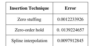
Table 1 shows results for each of the sample insertion methods and the FIR filter using convolution of 320 taps.
TABLEI
AVERAGE ERROR PER SAMPLE FOR THE CONVOLUTION FIR FILTER
Insertion Technique Error
Zero stuffing 0.0012233926
Zero-order hold 0. 0139224657
Spline interpolation 0.0097912845
In Fig. 9, frequency components of the FIR filter output signals before being trimmed are shown. It can be observed in the highest frequencies that the interpolated signal using splines presents the greater attenuation, whereas the signal with zero stuffing has significant components in the high frequencies. The signal inserted by the zero-order hold technique appears in the middle.
0 20 40 60 80 100 120 140 160
-0.2 0 0.2 0.4 0.6 0.8 1 1.2
Comparison of the interpolated signals in time domain
Time
x
'(
n
)
Zero stuffing Zero-order hold Splines Original signal
N
n
x
n
x
E
N
n
erp real
m
1int
(
)
Fig.9The output signal’s spectra for the convolution filter
In Fig. 10, the measured error for the comparator is shown. It is presented for each of the signals interpolated through filtering by convolution. In order to compare it to the original signal, the output signals of the filter have been trimmed to 160 samples.
Fig.10Comparison of the error for the three interpolated signals with the FIR filter using convolution
The program was carried out on a personal computer with a 3 GHz Pentium IV processor. On average, the time needed for the convolution filter process was 99.4908 ms.
0 50 100 150 200 250 300 350 400 450 500
10-10 10-8 10-6 10-4 10-2 100
Comparison of the interpolated signals in frequency domain
Frequency
X
'(
m
)
Zero stuffing Zero-order hold Splines
0 20 40 60 80 100 120 140 160
10-6 10-5 10-4 10-3 10-2 10-1
Error comparison
Samples
E
rr
o
r
IV.FASTFIRFILTERINGUSINGDFT
Since the convolution in the time domain corresponds to multiplication in the frequency domain, the scheme shown in the Fig. 11 can be used to realize the filtering. First, the spectra of the signals are obtained, which is reached by using the DFT for both the input signal xi(n) and the filter response h(k). Next, the multiplication is realized in the frequency domain and then, the IDFT is applied to return to the time domain, obtaining y(n). In several studies, it is demonstrated that these filters are faster than the filters that use convolution, whenever the output sequence size is greater than 30 [8].
Fig.11Block diagram for the implementation of the fast FIR filtering using the DFT
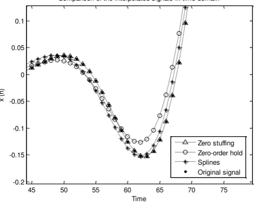
Fig. 12 shows results for the implementation of the DFT filtering with 160 points for each of the inserted signals.
Fig.12Zoom-in effect of the output signals of the fast filter using DFT
Applying a zoom-in from samples 45 to 75, see Fig. 12, the original signal appears within the triangle that represents the signal with zero stuffing. The measured error represented as the magnitude of the difference between the values of the interpolated functions and the original function, is shown in Fig. 13. Table 2 shows the average error per sample using fast filtering and Eq. 7.
45 50 55 60 65 70 75
-0.2 -0.15 -0.1 -0.05 0 0.05 0.1
Comparison of the interpolated signals in time domain
Time
x
'(
n
)
Fig.13Error comparison for the three interpolated signals using DFT-based fast filter
With the fast filtering method, the signal with zero-order hold and the signal with spline insertion report a smaller error than when using convolution. Nevertheless, the interpolated signal with zero stuffing appears to overlap the original signal, presenting a despicable error.
TABLEII
AVERAGE ERROR PER SAMPLE FOR THE CONVOLUTION FIR FILTER
Insertion Technique Error
Zero stuffing 0.0000000000
Zero-order hold 0.0113832780
Spline interpolation 0.0092012190
On average, the execution time for the fast filtering process using the DFT was 3.0353 ms.
V.RESULTS
Considering the filters implemented by convolution with a length of 320 taps, there is a reported average error of 0.001, 0.013 and 0.009 respectively for the techniques of zero stuffing, zero-order hold and spline interpolation. These results show an error that can be slowly reduced for higher-order filters. Using the DFT-based fast filter, the obtained average error is: 0.000, 0.011 and 0.009 respectively for the techniques of zero stuffing, zero-order hold and spline interpolation.
The frequency domain analysis for the output of the convolution FIR filter shows that the interpolated signal using spline has the best response in the higher frequencies. This characteristic can be important if a suitable filtering stage is not possible. On the other hand, the signal with zero stuffing insertion does not alter the signal in the passband. In this case the reconstruction with the DFT-based fast filter showed a perfect reconstruction. Comparing the execution time, the fast filtering process using the DFT was 37 times faster than the convolution based filter.
0 20 40 60 80 100 120 140 160
10-5 10-4 10-3 10-2 10-1
Samples
E
rr
o
r
Error comparison
VI.CONCLUSION
The analysis of the different interpolation techniques shows that the spline-based interpolation and the zero-order hold techniques have a relatively small reconstruction error. This takes into account high-frequency ranges, which can be desirable if a suitable filtering stage is not available. However, these two insertion techniques add frequency components in the passband range. On the other hand, the technique of zero stuffing does not add new frequency components in the passband, but their images can cause a problem if the quality of the filter is not appropriate.
Both, the filter using convolution and the DFT-based fast filter, execute interpolation with a relatively small error. Nevertheless, the latter shows better results when the zero stuffing insertion technique is implemented because it suppresses the images that are the primary weakness of this technique. Therefore, the insertion technique of zero stuffing together with DFT-based fast filtering is a recommendable choice due to its low reconstruction error and lower computation time in comparison to the convolution filter.
REFERENCES
[1] Neugebauer, O., “Astronomical Cuneiform texts. Babylonian Ephemerides of the Seleucid period for the motion of the sun, the moon and the planets”, London UK Lund Humphies, 1955.
[2] Ortega Aramburu, J. M., “Introducció a l'AnàlisiMatemàtica”, 2nd ed., Ed. Univ. Autònoma de Barcelona, 2002.
[3] Castillo Soria, F. R., Arellano Pimentel, J. J. , and Sánchez Sánchez, S.,“Statistical Approach to Basis Function Truncation in Digital
Interpolation Filters”, International Journal of Electrical and Electronics Engineering, Vol.4, Issue 3, 2010.
[4] Oetken, G.,“A new approach for the design of digital interpolating filters”, IEEE Transactions on Acoustics, Speech and Signal Processing, Vol. 27, Issue 6, January 2003.
[5] Schafer, R.W.,Rabiner, L., "A digital signal processing approach to interpolation," Proceedings of the IEEE , Vol.61, Issue 6, pp.692,702, June 1973.
[6] Aboul-Hosn, R.,and Bozic, S. M.,“Multirate techniques in narrow band FIR filters”, International Journal of Electronics, Vol. 71, Issue 6, 2007.
[7] Glasbey, C. A.,Van Der Heijden, G. W. A. M.,“Alignment and Sub-pixel Interpolation of Images using Fourier Methods”, Journal of Applied Statistics, Vol. 34, Issue 2, 2007.
[8] Lyons Richard, G.,“Understanding Digital Signal Processing”, 2nd ed., Ed. Prentice Hall, 2008.
[9] Fliege, N. J. , “Multirate digital signal processing: Multirate systems, Filter banks, and Wavelets”, John Wiley & Sons, 2000. [10] MitraS., “Digital Signal Processing: A Computer-Based Approach”, 3rd ed., McGraw-Hill International Press, 2005.
[11] Cormac Herley, and Ping Wah Wong, “Minimum Rate Sampling and Reconstruction of Signals with Arbitrary Frequency Support”, IEEE Transactions on Information Theory, Vol. 45, Issue 5, July 1999.
[12] Maday, Y., Cuong Nguyen, N., Patera, A. T., and Pau, G. S. H., “A general multipurpose interpolation procedure: the magic points”, Communications on Pure and Applied Analysis –Commun Pure Appl Anal., Vol. 8, Issue. 1, pp. 383-404, 2008.
[13] Mastroianni, G., Milovanović, G. V., and Notarangelo, I., “On an interpolation proces of Lagrange-Hermite type”, Publications de
L’InstitutMathematique Nouvelle série, tome 91(105), pp. 163–175, 2012.
[14] Turek, D. B., “Design of Efficient Digital Interpolation Filters for Integer Upsampling”, Master Thesis, Massachusetts Institute of Technology, June 2004.