Supernova Remnants as a Probe of Dust Grains in the Interstellar Medium

(1)

!!" ##$!%&$"$!'!"(#$$)*!!*

(2)

!" #

$%

%&!"

'()(

*+,-.

////////////////////////////////////////

0 11232 "4" "4"

(3)

!" #$ $ $## ## $!%%##&$ # $& ' !( $ $ #) %& * &+ %,# # '''!

($$- #.& & ( ! /& #$!# # $ ! &$ # $$ $ ( ## $ !

+$#$ # 0! / '''$ 1 2 # $$## !3 # $$$ 14!5! # !## 4!5!''2 --$ !

(4)

ACKNOWLEDGEMENTS

To my advisors, Steve Reynolds and Kazik Borkowski: Thank you, not only for teaching me about the universe, but also for your tireless efforts to turn me into a real scientist (or at least a reasonable first-order approximation of one). I will always appreciate the open doors that both of you had.

To my many collaborators: Thank you for your advice, patience, scientific contributions, and co-authorship of much of the work that has gone into this document.

To my friends in the Physics Department: Thank you for the countless opportunities to socialize and vent about classes, homework, research, and the general trials and tribulations that accompany graduate student life.

To my wife, Michelle Pearce: There are too many things to thank you for in this limited space. I will simply say this: Thank you for asking me to dance.

To my father, Steve Williams: Thank you for all of your never-ending love, support and interest in my work. You have been an ideal role model, and I could not ask for a better father.

(5)

iv

LIST OF TABLES

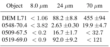
Table 3.1. Measured Fluxes and Upper Limits... 46

Table 3.2. Model Input Parameters... 47

Table 3.3. Model Results... 48

Table 4.1. Measured Fluxes... 58

Table 4.2. Model Inputs... 59

Table 4.3. Model Results... 60

Table 5.1. Aperture Parameters for Region Extractions ... 90

Table 5.2. MIPS 70/24 µm Regions Summary... 91

Table 5.3. MIPS 8/24 µm Regions Summary... 92

Table 6.1. Measured Fluxes... 128

Table 6.2. Line Fits ... 129

Table 6.3. Normalized Emission Line Fluxes ... 130

Table 8.1. Model Input Parameters... 187

(9)

viii

LIST OF FIGURES

Fig. 1.1. Hertzsprung-Russell Diagram, showing temperatures of stars vs. luminosity. Taken from http://www.le.ac.uk/ph/faulkes/web/stars/o_st_overview.html... 15

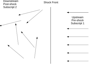
Fig. 1.2. Shockwave diagram, in the frame of reference of the shock. Arrows represent the velocities of particles upstream and downstream of the shock. In this frame, upstream material (at rest in the observer’s frame) races in towards the shock. The shock then randomizes the velocities of the particles, and

gives them a bulk velocity downstream of ! their initial velocity... 16

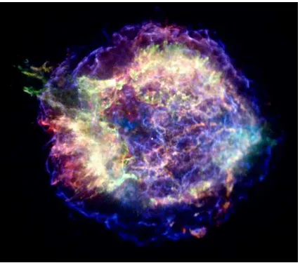
Fig. 1.3. SNR Cassiopeia A, seen in X-rays from the Chandra X-ray

Observatory. Image from http://chandra.harvard/edu/photo/2006/casa ... 17

Fig. 2.1. Background Subtracted Spitzer IRS spectra of warm dust in

SNR 0509-67.5, with model overlaid. The model will be discussed further in

chapter 7. Note absence of lines in spectrum. ... 29

Fig. 2.2. Diagram of the Spitzer Space Telescope, taken from

http://www.nasa.gov/missions/deepspace/f_spitzerbirth_prt.htm ... 30

Fig. 2.3. Figure 18 from Weingartner and Draine (2001), showing the size distribution of silicate (top) and carbonaceous grains (bottom) for the Large

Magellanic Cloud. For this work, I use their model “2.0 A.”... 31

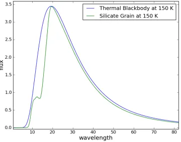
Fig. 2.4. Comparison of thermal blackbody at 150 K (blue) with single

silicate grain at 150 K (green)... 32

Fig. 2.5. Figure 17 from Draine (2003), showing grain temperature vs. time for 4 different grain sizes, heated by photons from the interstellar radiation

field. A similar stochastic heating process occurs for collisionally heated grains ... 33

Fig. 2.6. Figure 1a and 1d of Nozawa et al. (2006), showing the sputtering yield as a function of impinging particle energy for a variety of ions into carbonaceous

and SiO2 grains ... 34

Fig. 2.7. Figure 3a from Jurac et al. (1998), showing the enhancement in yield for protons of various energies, scaled to the yield for isotropic bombardment

of a flat surface (semi-infinite solid approximation) ... 35

(10)

ix

by protons with energy 10 keV. Rates used in code shown in blue, bulk solid approximation shown in green. Increase in rate from 10-2 – 10-1 µm due to enhancement of sputtering for small grains, dropoff short of ~10-2

µm due

to decreased energy deposition rate for energetic particles... 36

Fig. 2.9. The 70/24 µm MIPS flux from Kepler’s SNR (see Chapter 6) as a function of electron density, neand pressure, nekTe. The background

color scale indicates 70/24 µm ratio, as indicated by the color bar at right. Dashed lines are lines of constant temperature. The solid magenta

diagonal line at lower right indicates where the modeled shocks would become radiative, assuming solar abundance models and an age of 400 yr. Three solid curves are lines of constant 70/24 µm MIPS flux ratios, 0.30, 0.40, and 0.52 (from top to bottom). Position of a Balmer-dominated fast shock is marked by a star. There are many combinations of density and temperature

that can yield an identical 70/24 µm flux ratio... 37

Fig. 2.10. Spitzer IRS data of “faint” region (see Chapter 8) of 0509-67.5, overlaid with 90% confidence limits from model fit. The best-fit density for this data was np= 0.88 cm-3, and the 90% confidence lower and upper

limits are 0.7 and 1.0 cm-3, shown I green and blue, respectively. !2 statistics were only performed in the region from 21-32 µm, where

signal-to-noise was strongest... 38

Fig. 3.1. Top row: DEM L71 at 24 and 70 µm, H", and X-ray (red, 0.3 – 0.7 keV; green, 0.7 – 1.0 keV; blue, 1.0-3.5 keV; smoothed with 1 pixel Gaussian). Second row: 0548-70.4 with red, 24 µm; green, IRAC 8.0 µm; blue, IRAC 5.8 µm; 70 µm, H", and X-ray image as for DEM L71, smoothed with 2 pixel Gaussian. Third row: 0509-67.5 at 24 µm, H", and X-ray: red, 0.3 – 0.7 keV; green, 0.7 – 1.1 keV and blue, 1.1 – 7.0 keV, Bottom row: 0519-69.0, as in third row. Half-arcminute

scales are shown for each SNR... 49

Fig. 4.1. Top row, from left to right: N132D at 24 and 70 microns (the region of interest at 70 microns is marked on the iamge), in the X-rays (broadband, Chandra image) and in the optical (overlay of MCELS images, with [S II], H-alpha and [O III] marked in red, green, and blue, respetively). Second, third, and fourth rows show the same sequence for N49B, N23, and 0453-68.5, respectively. One arc-minute scales

are shown on the 24 µm images... 61

(11)

x

Scaling is set to a compromise level to show the overall structure to best advantage. The 24 µm image is by far the deepest and most detailed

of the Spitzer images. ... 93

Fig. 5.2. A six-panel color figure concentrating on the IRAC images and their comparison to other wavelength bands. Panel a shows a three-color IRAC image with 8 µm in read, 5.6 µm in green and 3.6 µm in blue. Panel b is similar, but for 5.6 µm in red, 4.5 µm in green, and 3.6 µm in blue. The orange color of the SNR filaments indicates emission in both 4.5 and 5.6 µm, but only from the brightest filaments seen at 8 µm. Panel c is a difference image of 8 µm minus 5.6 µm, scaled to show the extent of faint emission at 8 µm. Panel d shows the 4.5 µm minus 3.6 µm difference image. Panel e shows the 24 µm MIPS image from Fig. 5.1 to the same scale as the other images. The 8 µm image closely tracks the brightest regions at 24 µm. Panel f shows the soft band (0.3 – 0.6 keV) Chandra image from archival data, which again looks astonishingly like the 8 µm image in panel c. All images

are aligned and scaled exactly the same... 94

Fig. 5.3. A six-panel color figure concentrating on the MIPS images and their comparison to other wavelength bands. Panels a and b show the MIPS 24 µm data with a hard stretch and a soft stretch, respectively, to show the full dynamic range of these data. Panel c shows the MIPS 70 µm data after running through the GeRT software to improve the appearance of the background. Panel e shows the MIPS 160 µm data for the same field of view, although no SNR emission is actually seen at this wavelength. Panel d shows the star-subtracted H" image from Blair et al. (1991). Panel f shows a three-color representation of the Chandra

data for Kepler, with the red being 0.3 – 0.6 keV (as in Fig. 5.2f), green

being 0.75 – 1.2 keV, and blue being 1.64 – 2.02 keV ... 95

Fig. 5.4. SED apertures selected for assessing the bright NW radiative

emission and the sky background, projected on the 24 µm image ... 96

Fig. 5.5. Background subtracted SED 55-95 µm spectrum of the NW

region of Kepler’s SNR, as indicated in Figure 5.4... 97

(12)

xi

image was used to subtract stars from this image. See text for details ... 98

Fig. 5.7. This figure shows the object and background extraction regions selected for determining ratios between 24 and 70 µm (panels a and b) and between 8 and 24 µm (panels d and e). For reference, the regions are also projected onto the optical H" image from Blair et al. (1991) in panels c and f. Note that the images shown in panel a and d are the versions that have been convolved to the lower resolution image. Also, panel b shows the original (non-GeRT-corrected) 70 µm image. The labels

are used in the text and Tables 5.2 and 5.3... 99

Fig. 5.8. A ratio image of the 70 µm and 24 µm data, where only the regions with significant signal have been kept. The color bar provides an indication of the measured ratio, ranging from 0.28 to 0.9. A simple contour from the 24 µm image is shown for comparison. Note the lower values of the ratio in the regions of brightest emission, indicating

they are somewhat warmer. ... 100

Fig. 5.9. The 70/24 µm MIPS flux ratio as a function of electron density and pressure for plane shock dust models described in the text.The

background color scale indicates 70/24 µm ratio, as indicated by the color bar at right. Dashed lines are lines of constant temperature. The solid magenta diagonal line at lower right indicates where the modeled shocks would become radiative, assuming solar abundance models and an age of 400 yr. Three solid curves are lines of constant 70/24 µm MIPS flux ratios, 0.30, 0.40, and 0.52 (from top to bottom). Position of a Balmer-dominated fast shock

is marked by a star... 101

Fig. 6.1. Images of PWN 0540-69.3. Each image is approximately 100 arcseconds across. Left to Right, Top to Bottom: IRAC Chs. 1-4 (3.6, 4.5, 5.6, and 8.0 µm, respectively), MIPS 24 µm, Chandra broadband X-ray image. The location of the PWN is marked with a circle in the IRAC Ch. 1

image, and X-ray contours are overlaid on the IRAC Ch. 4. image ... 131

Fig. 6.2. Coverage of IRS slits overlaid on a MIPS 24 µm image... 132

Fig. 6.3. The short-wavelength, low-resolution spectrum of the PWN. Local background has been subtracted as described in the text. Dashed line is source + background; dotted line is background, solid line is the spectrum

of the source only... 133

(13)

xii

are the same as in Figure 6.3 ... 134

Fig. 6.5. The high-resolution spectrum of the PWN, with no background

subtraction. Measured lines are marked, along with a dust feature at ~11 µm ... 135

Fig. 6.6. An example of our two-component fit to the lines identified in the high-resolution spectrum of the PWN. [Ne III] is clearly seen to have two components. Noisy pixels were clipped out for the fitting, but were left

in this image to show their relative level of contribution... 136

Fig. 6.7. A cartoon sketch of our general picture discussed in section 6.4.1. Not to scale. FS refers to the forward shock from the SN blast wave, at a radius of 30”. RS refers to the reverse shock, which has not yet been observed, and is at an unknown position between 10 and 30” from the pulsar. [O III] refers to the extent of the halo of material that has been photoionized, and is seen in optical images to extend to 8”. PWN refers to the edge of the shock driven by the pulsar wind, and is located at a radius of 5”. Interior to this shock, ejecta material has fragmented into clumps. The PWN as a whole is observed to have a redshifted velocity as reported in previous optical observations, possibly resulting from a pulsar kick. This is also the region where relativistic particles from the pulsar create observed synchrotron

emission; see discussion in text. ... 137

Fig. 6.8. Hubble Space Telescope WFPC2 image of PWN 0540-69.3, from Morse et al. (2006). Colors are: Blue – F791W continuum; Green –

F502N [O III]; Red – F673N [S II]... 138

Fig. 6.9. The background subtracted low-resolution spectrum of the PWN is plotted as the solid line, with the radio synchrotron component shown

as a dashed line. A clear rising excess can be seen longward of 20 µm ... 139

Fig. 6.10. Broadband spectrum of 0540. Radio points (diamonds):

Manchester et al. (1993). IR points (triangles): our MIPS and IRAC fluxes. Optical points (circles): Serafimovich et al. (2004). X-rays (solid line):

Chandra (Kaaret et al. 2001). Dashed line: model described in text... 140

Fig. 7.1. Size distribution of porous grains in the ISM, from Clayton

et al. (2003)... 154

Fig. 7.2. Size distribution of porous grains in the ISM, from Mathis (1996). Eq. (3) of his paper gives the functional form of the distribution as

(14)

xiii

"2 = 0.437 µm, and "3= 50 µm-2... 155

Fig. 7.3. The impact of proton heating of grains for slow (~1000) and fast (~ 3000 km s-1) shocks. For slow shocks, the difference between proton heating and no proton heating is hardly noticeable, but for fast shocks it becomes quite significant. Top: Thermal spectrum of warm grains heated behind slow non-radiative shock. Blue curve shows spectrum with Tp = 1 keV, Te = 0.5 keV, Green curve shows Tp = 0 keV, Te = 0.5 keV. Bottom: Same as top, but for fast non-radiative shock. Blue curve shows spectrum with Tp = 20 keV, Te = 1 keV, Green curve shows Tp = 0 keV, Te =

1 keV ... 156

Fig. 7.4. Comparison of model spectra from 10 – 200 µm for silicate grain size distribution of varying porosity. Blue: Compact silicate grains; Green: 10% porous silicate grains; Red: 25% porous; Cyan: 50% porous. Size distribution of Clayton et al. (2003) assumed, heating model (identical plasma conditions for all grain populations) described in text. Sputtering

is neglected to highlight differences by heating only... 157

Fig. 7.5. Stopping power of a proton in silicon dioxide (SiO2) as a function

of proton energy. Taken from the NIST PSTAR database (see text) ... 158

Fig. 7.6. Stopping power of astronomical silicate, as calculated from Bragg’s Rule (see text). For comparison, the stopping power of SiO2 obtained from

the NIST PSTAR database is also shown ... 159

Fig. 7.7. Projected range of a proton for MgFeSiO4 as a function of energy. Solid curve is calculation described in text; dashed curve is approximation of Draine & Salpeter (1979) that is valid at E < 100 keV. The slight discrepancy at low energy is result of approximations in Bragg’s

rule and in Draine & Salpeter (1979)... 160

Fig. 7.8. $p (a,E), the fractional energy deposited by a proton into a silicate grain as a function of particle energy. From bottom-left (blue) to top-right (black), curves represent grains of radius 0.001, 0.003, 0.01, 0.03, 0.3 and

1.0 µm... 161

Fig. 7.9. Zeta function for a single grain of 0.05 µm radius. Solid curve is calculation described in text, dashed curve is approximation of Dwek &

Werner (1981) (see text)... 162

(15)

xiv

in this work to approximations from Draine & Salpeter (1979) & Dwek & Werner (1981) for an impinging particle energy of 100 keV, as a function

of grain radius ... 163

Fig. 7.11. Comparison of spectra produced in dust heating model for protons of 100 keV. Solid line: spectrum assuming proton projected

ranges calculated in Section 7.5. Dashed line: spectrum assuming analytical approximation to proton projected range from Draine & Salpeter (1979).

Electron heating (Te = 2 keV) is included in this model ... 164

Fig. 7.12. Ratio of spectra from Figure 7.11 ... 165

Fig. 7.13. 3-color image of the P7 region of the Cygnus Loop. Red: H";

Green: Spitzer 24 µm; Blue: Chandra X-ray... 166

Fig. 7.14. Spitzer 24 and 70 µm images of the Cygnus Loop, with analysis

regions overlaid... 167

Fig. 7.15. 70/24 µm flux ratio as a function of sputtering timescale for a temperature of Tp = Te = 0.3 keV, appropriate for the Cygnus Loop. Solid black curve includes effects from both thermal and non-thermal sputtering,

dashed black line includes only thermal sputtering ... 168

Fig. 7.16. Sputtering rate as a function of grain radius, where sputtering is done by protons with energy 10 keV. Rates used in code shown in blue, bulk solid approximation shown in green. Increase in rate from 10-2 – 10-1 µm due to enhancement of sputtering for small grains, dropoff short of ~10-2µm due

to decreased energy deposition rate for energetic particles. Same as Figure 2.8. ... 169

Fig. 7.17. Sputtered fraction, by mass, for grains as a function of sputtering timescale. Solid black line: Silicate grains (MgFeSiO4); Dashed line: Graphite

grains. Plots are for dust in the ISM of the Milky Way. ... 170

Fig. 7.18. Same as Figure 7.17, but for post-shock proton temperatures of 3

and 10 keV... 171

Fig. 8.1. Top: MIPS 24 µm image of SNR 0509-67.5, overlaid with regions of spectral extraction as described in text, where magenta region is “faint” region and cyan is “bright.” Bottom: MIPS 24 µm image of SNR 0519-69.0. Green bar on both images corresponds to 30”. FWHM of MIPS 24 µm PSF

(16)

xv

Fig. 8.2. 14 – 35 µm IRS spectrum of the “faint” region of 0509, overlaid

with model fit... 190

Fig. 8.3. 14 – 35 µm IRS spectrum of the “bright” region of 0509, overlaid

with model fit... 191

Fig. 8.4. 14 – 35 µm IRS spectrum of SNR 0519-69.0, extracted from a slit placed across the middle of the remnant, free of emission from the bright

knots seen in the 24 µm image; model overlaid. ... 192

Fig. 8.5. Top: XMM-Newton RGS spectrum of 0509-67.5, from 5 – 23 angstroms. Bottom: RGS spectrum of 0519-69.0, from 5 – 27 angstroms;

models overlaid in both as described in text... 193

Fig. 8.6. Star-subtracted H" images of 0509 (left) and 0519 (right). Note

(17)

1

1. Introduction to Supernovae and Supernova Remnants

Supernova explosions are among the most energetic events in the universe since the Big Bang, releasing more energy (∼ 1051−1053 ergs) than the Sun will release over its entire lifetime. They are the cataclysmic ends of certain types of stars, and are responsible for seeding the universe with the material necessary to form other stars, planets, and life itself. We owe our very existence to generations of stars that lived and died billions of years ago, before the formation of our Sun and solar system. The processes of stellar evolution continue to occur today, with typical galaxies like the Milky Way hosting several super-novae per century, on average. The study of supersuper-novae and the role they play in shaping the evolution of star systems and galaxies is truly an exploration of our own origins. Super-nova remnants (SNRs), the expanding clouds of material that remain after the explosion, spread elements over volumes of thousands of cubic light-years, and heat the interstellar medium through fast shock waves generated by the ejecta from the star.

1.1. Stellar Evolution

Any study of SNRs must begin with the processes which cause a star to go supernova. Stars come in all sizes and colors (where the color of a star is related to its temperature), but virtually all stars live out their lives in a similar fashion. They spend the majority of their lives fusing hydrogen in their cores into helium, a process which releases energy. This process is not particularly efficient in stars; nevertheless, the sheer mass of available ma-terial to burn means that stars shine at a roughly constant brightness for millions, billions, even tens of billions of years. The life expectancy of a star is a rather sensitive function of its initial mass. This relationship is perhaps counterintuitively inverted, such that the more massive a star is, the shorter its lifetime. (This is due to the fact that massive stars, while having much more fuel to burn, fuse it at a much faster rate than do low-mass stars). Stars that are on the hydrogen burning phase of their lives are said to be on the “main sequence,” a reference to the Hertzsprung-Russell diagram seen in Figure 1.1.

(18)

2

provide the necessary counter-balancing force. The fate of a star at this point depends on its mass, with high and low-mass stars following very different paths.

1.1.1. Low-Mass Stars

Stars that begin their main-sequence lives with a mass of less than about 8 solar masses (M!, whereM!is∼1.99×1033grams) will spend the majority of their lives in the

hydro-gen burning phase. When their hydrohydro-gen runs out, they will swell into red giants, increasing in volume by a factor of>1000. (The smallest of stars, with masses <0.5M!, will not

even have enough power to reach this stage). The red giant phase is typically characterized by a helium core surrounded by a hydrogen burning shell. When the core contracts and heats to temperatures above∼ 108 _{K, helium burning will begin, fusing helium to carbon}

via the triple-alpha process. The core of the star that remains typically cannot fuse much beyond carbon and oxygen, and collapses further when the helium supply is used up. The outer layers of the star are ejected, creating the misleadingly named “planetary nebula.” Collapse continues until the degenerate pressure of electrons in the plasma is sufficient to balance the gravitational forces, creating a “white dwarf” star. A typical white dwarf has a mass of∼0.6−0.7M!contained in a volume about the size of the Earth (R∼6000km),

which leads to an average density for a white dwarf of ∼ 106 _{g cm}−3_{. White dwarfs are}

typically very stable (although see section 1.2), and will exist as burned-out remnants of once bright stars indefinitely.

1.1.2. High-Mass Stars

Stars above ∼ 8 M! are hot enough at their cores to fuse hydrogen into helium,

helium into carbon, carbon into oxygen, neon, silicon, sulfur and other elements, stepping up the periodic table. Once iron (element 26) is reached, though, it no longer becomes energetically favorable for the fusion process to continue. The iron core collapses in upon itself on timescales of the order of a second, sidestepping electron degeneracy pressure by eliminating electrons, combining them with protons to form neutrons. Once nuclear density (∼1015_{g cm}−3_{) is reached, the degeneracy pressure of neutrons is sufficient to halt}

(19)

3

from the core bounces off of this now hard core, ejecting the outer layers of the star in a fantastic explosion known as a “core-collapse supernova.” The proto-neutron star forms a neutron star, a stellar remnant of order 1 M! and R ∼ 10km, with an average density

of ∼ 1015 _{g cm}−3_{. For highly massive stars, it is possible that even neutron degeneracy}

pressure cannot halt the collapse of the core, and a stellar-mass black hole is formed.

1.2. Supernova Classification

As in many sciences, observations of events or objects in astronomy often precede theoretical explanations for said events. However, unlike in most disciplines, astronomers normally do not have the means to conduct laboratory tests of observed phenomena. This often leads to a significant time delay between the observation of and the theoretical de-scription of a given event. As a result, the field is riddled with examples of “historical inac-curacies” when it comes to naming and classification schemes. A prime example of this is the supernova classification scheme, where astronomers classify supernovae as “Type I” or “Type II” based solely on the existence of hydrogen lines in their spectra; Type I SNe show no hydrogen lines, Type II do. It was only later realized that vastly different processes can be responsible for this bit of observational data.

1.2.1. Type Ia

The vast majority of stars in the galaxy are <8M!, meaning (see Section 1.1.1) that

they are destined to end their lives as white dwarfs. However, many stars in the galaxy are also part of binary (or even triple) systems. If a white dwarf is contained in a binary system with a companion star that enters its red giant phase (or has even slightly evolved off the main sequence), and the separation between the stars is sufficiently close, the white dwarf can gravitationally strip matter from its companion. Mass transfer occurs between the two stars, with the white dwarf growing in mass via an accretion disk. White dwarfs can only exist up to the “Chandrasekhar limit,” and a white dwarf pushed over this limit (∼1.4M!)

(20)

4

at speeds of∼ 10,000 km s−1_{, releasing about 10}51 _{ergs of kinetic energy. Type Ia SNe}

leave behind no compact remnant, and their light curve, i.e. the brightness of the supernova as a function of time, is primarily powered by the radioactive decay chain of nickel-56 to cobalt-56 to iron-56. Their light curves peak a few days after explosion, then slowly fade over the course of a few months. Since all white dwarfs are thought to explode at an identical mass via the same mechanism, their light curves are quite similar in peak brightness, and can be used as a “standard candle” to determine extragalactic distances. Type Ia spectra show no hydrogen because white dwarfs are made mostly of carbon and oxygen, nearly all of which is burned to nickel in the explosion.

1.2.2. Type II

Type II supernovae result from the deaths of massive stars, greater than 8 M!, but

generally not more than ∼ 25−30M!. These stars end their lives as core-collapse SNe

(CCSNe), ejecting their outer layers (5-25 M!) at a velocity of ∼ 5,000 −10,000 km

s−1_{. Coincidentally, they yield roughly the same amount of kinetic energy (}_∼ ₁₀51 _ergs)

as do type Ia SNe, but their overall energetics are much greater. Ninety-nine percent of the energy released in a CCSN is carried off by neutrinos. Type II SNe leave behind a neutron star that is typically∼1.4M!with an initial temperature (kT) of several MeV. Type II SNe

can be further divided into subclasses based either on the shape of the light curve or the spectrum (e.g. IIP, IIL, IIb, IIn, etc.). They show hydrogen lines in their spectra because the outer atmosphere of the star at the time of explosion still contained a significant amount of hydrogen.

1.2.3. Type Ib and Ic

(21)

5

are believed to be the result of stars with a progenitor mass of >_∼ 30M!, although this

number could be lower in binary systems. They leave behind neutron stars and stellar-mass black holes. As with type II SNe, most of their energy is carried off in neutrinos, and their light-curves, both in peak brightness and in shape, can vary greatly.

1.3. Astrophysical Shocks

Shock waves, propagating supersonic disturbances, occur commonly in all sorts of astro-environments throughout the universe, where conditions are unlike those found on Earth. Densities in the interstellar medium (ISM) are on the order of a few particles per cubic centimeter, six orders of magnitude less than can be produced in the best laboratory vacuum systems. Sound speeds in the ISM are usually on the order of a few km s−1_,

rel-atively slow by astrophysical standards. The shock waves generated by a supernova are an excellent example of a strong shock, with shock speeds often being several thousand times the speed of sound in the ISM. These shock waves compress, sweep, and heat inter-stellar material. In fact, supernova shock waves are one of the main sources of heating of the interstellar medium, as well as the mechanism for distributing material throughout the universe.

The following is a mathematical description of a shock wave, beginning with the Rankine-Hugoniot Conditions, given by

ρ1v1 =ρ2v2, (1)

ρ1v12+p1 =ρ2v22+p2, (2)

1 2v

2

1 +E1+

p1

ρ1 = 1

2v 2

2 +E2+

p2

ρ2

, (3)

(22)

6

post-shock gas. These equations are written in the frame of reference of the shockwave (see Figure 1.2). In particular, this means that v1 is not zero (in fact, v1 = −vshock) even

though there is no motion in front of the shock in the observer’s frame.

Equation (1) is the conservation of mass across the shock, while Equation (2) shows that the sum of the ram pressure, ρv2_{, and thermal pressure} _p _{must be equal across the}

shock. This amounts to a conservation of momentum. Equation (3) is the conservation of energy (kinetic, internal, and thermal).

The volume of the gas is given by V, such that dV =d1_ρ. Thus dE = −pdV =

−Kργ_d1

ρ, which can be integrated to obtain E =

1

γ−1

p

ρ. The thermodynamic relation

be-tween pressure and density isp = Kργ _where_K _{is a constant (although it is not constant}

across the shock) andγ is the polytropic index of the gas.γ varies depending on the prop-erties of the fluid and is given by:

γ = 5/3for non-relativistic monoatomic gas (as is generally found in the ISM),

γ = 4/3for relativistic monoatomic gas,

γ = 7/5for non-relativistic diatomic gas.

Using this, eq. (3) becomes

1 2v

2

1+

1

γ−1

p1 ρ1 = 1 2v 2 2+ 1

γ−1

p2

ρ2

(4)

Using the Rankine-Hugoniot conditions, it can be shown that

ρ2

ρ1

= (γ+ 1)p2+ (γ−1)p1 (γ+ 1)p1+ (γ−1)p2

= v1

v2

. (5)

This is the shock jump condition for density, giving the compression ratio, which relates density (and thus fluid velocity) ahead of the shock and behind the shock. In the limit of strong shocks, that is,p2 $p1, orM $1, whereM is the Mach number (defined

asvshock/vsound), we can neglect the pre-shock pressure so that

ρ2

ρ1

= γ+ 1

(23)

7

forγ = 5/3. In the limit of a strong shock, we also have

p2

p1

= 2ρ1v 2 1

p1(γ+ 1), (7)

or

p2 = 2ρ1v12

γ+ 1. (8)

The gas is also governed by the ideal gas law such thatp2 =n2kT2, where k is Boltzmann’s

constant. So

p2 = 2ρ1v12

γ+ 1 =

3 4ρ1v

2

1 =n2kT2, (9)

wheren = _mρ = total particle number density, andmis the mean mass per particle. Thus,

p2 = 2ρ1v12

γ+ 1 =

3 4ρ1v

2

1 =

ρ2

µmp

kT2, (10)

wheremp is the mass of a proton, equal to 1.67×10−24 grams. Further simplifying, we

have

kT2 = 3 16µmpv

2

s, (11)

whereµmp is the mean mass per particle behind the shock (for a fully ionized plasma of

cosmic abundances, µ ∼ 0.6). This is the temperature behind a shock, where vs = v1

is the shock speed. kT2 is the “shock temperature,” which is the average of proton and

electron temperatures. In the absence of heating of electrons at the shock (and assuming no sharing of energy between protons and alpha particles), the initial temperature ratio be-tween protons and electrons,Tp/Te, is just the ratio of the masses of protons and electrons, mp/me = 1836. Behind the shock, these temperatures equilibrate to bring down Tp and

bring up Te, but the timescale for equilibration is long, and is a function of the post-shock

(24)

8

electrons at the shock, with near full equilibration seen in old remnants like the Cygnus Loop (vs∼300−400km s−1) and little equilibration seen in younger remnants like Tycho

(vs ∼2000km s−1).

For supernova shock waves of order a few thousand km s−1_{, this shock temperature}

will be of order 10 million K. Thus, shocked gas will radiate thermal emission at X-ray en-ergies, however, other emission mechanisms also operate in SNRs. Non-thermal emission from synchrotron radiation is often seen near the forward edge of the shock wave in young SNRs, and line emission from ionized elements is common in the shocked ejecta. Shocks in SNRs are “collisionless,” in that collisions between particles are extremely rare, mean-ing that particle interactions are mediated by magnetic fields. This is a good approximation when the Coulomb mean free path is much greater than the gyroradius of the thermal par-ticles.

1.4. Supernova Remnants

The expanding material ejected from the star, rich in heavy elements like oxygen, silicon, and iron, as well as the shock wave which it drives into the ISM is known as a supernova remnant (SNR). Figure 1.3 shows Cassiopeia A, an example of a young (∼

330 yrs) SNR in our own galaxy. Although Cassiopeia A is known to have resulted from a CCSN, it is generally difficult to tell the type of SN only by looking at the remnant. SNRs remain visible for thousands, often tens or hundreds of thousands of years before dissipating their energy into the ISM. The life of a SNR can be thought of as consisting of four phases.

1.4.1. Free Expansion Phase

Immediately following the explosion, the ejecta from the supernova race out into the ISM at speeds of∼ 10,000km s−1_{, driving a strong shock at the leading edge. Since the}

(25)

9

1.4.2. Reverse-Shock Phase

As the shock continues to expand and sweep material it encounters, the accumulated mass becomes non-negligible, and gradually causes the shock to slow. The ejecta behind the shock, however, are still traveling at a free-expansion velocity, and slam into the decel-erating material ahead of it. This causes a reverse shock to form. Initially, this “reverse” shock moves inward only in the Lagrangian shock frame, and still moves outward in the observer’s frame. The reverse shock, however, eventually “turns around” and moves in-ward in the frame of reference of the observer. It typically takes of order hundreds of years for this transition to occur. When the ejecta are in free-expansion cooling is almost en-tirely adiabatic. While this adiabatic cooling is effective in lowering the temperature of the ejecta, energy is still conserved for the system because the energy is not radiated away. Upon encountering the reverse shock the ejecta are heated, like the ISM at the forward shock, to very high temperatures, thus radiating strongly in X-rays. This radiative cooling is still relatively inefficient, and most of the energy of the SNR+ISM system is conserved. The duration of the reverse shock phase can last tens to thousands of years.

1.4.3. Sedov-Taylor Phase

Once the mass swept-up by the forward shock greatly exceeds the ejecta mass, the remnant enters the Sedov-Taylor phase (often known simply as the Sedov phase). The reverse shock has propagated all the way back through the ejecta and dissipated, and the remnant can be described by a self-similar solution (Sedov 1959). The similarity variable can be derived by dimensional analysis, and is given by

ξ=R(ρ/Et2₎1/5 ₍₁₂₎

(26)

10

R ∝(E

ρ)

1 5t

2

5. (13)

It can be immediately seen from this that the shock velocity is given by

Vs= dR

dt =

2R

5t . (14)

The Sedov phase lasts for thousands to tens of thousands of years after the explosion.

1.4.4. Radiative Phase

The shock continues to sweep up material and decelerate, eventually reaching a point where the forward shock speed is only a few hundred km s−1_{. At this point, the temperature}

of the post-shock gas drops below 106 _{K, and radiative cooling of the gas becomes}

impor-tant. Cooling of the gas is a runaway process, as the more it cools, the more the cooling rate increases. As the gas temperature drops further, the material once again becomes visible in optical radiation. The forward shock is driven mostly by momentum conservation at this point, and eventually will turn sub-sonic and dissipate into the ISM.

1.5. Radiation Mechanisms in SNRs

SNRs radiate throughout the electromagnetic spectrum. In radio waves, the emis-sion is entirely non-thermal in origin, resulting from synchrotron radiation from relativistic electrons spiraling around magnetic fields. Synchrotron emission is characterized by a fea-tureless power-law spectrum, where the radio flux, Sν is given bySν ∝ ν−α, where ν is

the frequency andαis the spectral index, which depends on the energy distribution of the electron population.

(27)

11

Fe.

At optical wavelengths, radiation prior to the radiative phase comes primarily from hydrogen Balmer lines (transitions from n ≥3→ 2), such as Hα, λ= 656.3 nm, and Hβ,

λ= 486.1 nm. This requires the presence of neutral hydrogen ahead of the shock, which is much more easily attained in the case of a type Ia SN, since CC SNe generally ionize the surrounding medium, either with ionizing radiation from the progenitor, or a flash of ultra-violet (UV) radiation at the moment of explosion. Charge exchange between slow neutral atoms and fast protons behind the shock produces fast-moving neutral atoms, generating a broad Hα line, with a narrow component arising from stationary neutral atoms in the post-shock medium. During the radiative phase, strong optical lines are seen from a variety of atomic species, most strongly from Hα and singly-ionized sulfur ([S II]). Ultraviolet (UV) emission from SNRs is also produced, generally from higher ionization states than in optical.

Soft X-rays (0.1-2 keV) are generally thermal in origin, and in SNRs are often domi-nated by line emission from highly ionized elements. Typically, elements that emit X-ray line emission have been stripped of all but one or two electrons, making them “hydrogen-like” or “helium-like.” As with optical and infrared lines, downward transitions of electrons to lower energy levels causes emission of a photon whose energy is equal to the transition energy between the electron’s bound states. For elements that still contain multiple elec-trons, the transitions between energy states become more complicated, and generally gener-ate numerous lines which are smeared together by current X-ray spectroscopic technology. Continuum emission, detailed below, is also observed at these energies.

(28)

12

Non-thermal emission in SNRs arises from synchrotron emission identical to that seen in radio waves, but from much more energetic electrons. The maximum photon energy in keV of an electron with energyEis given by

hν = 1.93(E/100T eV)2(B/10µG)keV. (15)

In order to produce synchrotron emission in the 2-10 keV range, electrons with energies of 100-200 TeV are required. Because this is well beyond the particle thermal energies for even a fast shock, another process must accelerate particles to high energies in remnants where non-thermal emission is conclusively identified. The origin of these high-energy cosmic-ray electrons is discussed in the next section.

At gamma-ray energies, emission can be produced by one of three processes; two of which are leptonic in origin, one of which is hadronic. Bremsstrahlung, both thermal and non-thermal in origin, can account for photons of all energies, up to TeV emission. Inverse-Compton scattering from relativistic electrons off of cosmic microwave background or far-infrared photons can upscatter the photons to very high energies. The only known hadronic source of gamma-ray emission is the decay of neutral pions, orπ0 _{particles, into}

two gamma-ray photons. This process occurs 98.7% of the time in π0 _{decays. The} _π0

particles themselves are produced in collisions between cosmic-ray protons and thermal protons, as well as protons and alpha particles in the pre-shock gas. The minimum pion energy required to produce a gamma-ray of energy Eγis given by

Emin(π) =Eγ+ (m2πc4/4Eγ) (16)

To produce high energy gamma rays (> 1GeV), the last term on the right becomes neg-ligible, and the minimum pion energy needed is roughly equal to the gamma-ray energy observed.

(29)

13

1.6. Cosmic-Ray Acceleration in SNRs

Cosmic-rays are highly energetic particles, typically protons, alpha particles, and nu-clei of heavier elements, with a small percentage of the population consisting of electrons, streaming through space at relativistic speeds. They can either be detected directly (at lower energies), or indirectly through interactions with atoms in the Earth’s upper atmosphere (at high energies). Upon the collision of a cosmic-ray with our atmosphere, a shower of particles (mostly containing pions) is produced. These pions decay further into elec-trons, posielec-trons, muons, neutrinos, and photons, and can be detected from ground-based Cherenkov telescopes. Such telescopes can even reconstruct the events to determine the location in the sky from which the cosmic-ray came. Unfortunately, this location is not indicative of the original source of the particle. Since cosmic-rays are charged particles, they gyrate around the magnetic field lines of our Galaxy, and are essentially randomized by the time they reach Earth. This leads to a mystery: from where do cosmic-rays come?

1.6.1. Cosmic-Ray Sources

The fact that synchrotron emission is observed in radio waves for every Galactic SNR known shows that, at the very least, electrons are efficiently accelerated to energies of a few GeV. If electrons are accelerated, protons and ions should be accelerated as well. This, unfortunately, is a difficult thing to observationally verify, because the synchrotron radia-tion from relativistic protons is orders of magnitude weaker than from electrons spiraling around a magnetic field. Gamma-ray production via the decay ofπ0_{particles, discussed in}

the previous section, requires that protons at GeV energies exist. Unambiguous detection of this hadronic gamma-ray signal in SNRs would provide the observational confirmation that such acceleration of ions is taking place. Searches for this signal are currently underway.

Detection of non-thermal synchrotron emission at X-ray energies is a clear indication that the shock is accelerating electrons beyond TeV energies. If the shocks are equally as efficient at accelerating protons, this could account for the galactic cosmic-ray spectrum to energies up to∼1015_{eV. Cosmic-rays at much higher energies have been detected, but it is}

(30)

14

If supernova shock waves are efficiently accelerating cosmic rays, then the equations detailed in Section 1.3 are no longer valid, since escaping cosmic rays can rob the shock of energy. This leads to a higher compression ratio (r ≡ ρ2/ρ1), and a lower post-shock

temperature. Even if no cosmic rays escape, the compression ratio can still be increased if relativistic particles dominate, since r→7 asγ → 4₃.

1.7. Summary

Supernovae represent the end of a star’s life, but in the process of dying, elements that will go on to form future generations of stars and planets are spread throughout the galaxy. The universe is nearly 14 billion years old, old enough that every cubic centimeter of a galaxy like the Milky Way has been overrun numerous times by shock waves produced by SNe. They represent one of the main feedback mechanisms in the evolution of a galaxy, shaping and recycling products in the ISM.

(31)

15

(32)

16

(33)

17

(34)

18

2. Infrared Emission from Young Supernova Remnants

IR emission from SNRs is predominantly thermal emission from warm dust grains, heated via collisions with hot electrons and ions in the post-shock gas. Although IR line emission can become strong once a shock reaches its radiative phase, it is virtually non-existent in fast, non-radiative shocks, as Figure 2.1 shows. This work focuses on emission from these non-radiative shocks, which typically persist for hundreds or thousands of years in SNRs before becoming radiative.

2.1. What is Dust?

Dust grains in the ISM are not like the dust that accumulates on top of TVs and coun-tertops. ISM grains are microscopic, ranging in size from molecules of a few atoms to small solid bodies, several microns (µm, where 1 µm = 10−6_{meters) in radius. Grains are made}

up of various elements, most notably carbon (which can exist in either crystalline forms like graphite or in amorphous forms), oxygen, silicon, magnesium, and iron. Polycyclic aromatic hydrocarbons (PAHs) have also been spectroscopically identified as residing in the ISM. These molecules are similar to PAHs produced on Earth, typically as byproducts of fuel burning. PAHs consist of aromatic rings of carbon with hydrogen atoms at their edges. On average, about 0.1-1% of the mass of the ISM is contained in dust grains, with the remainder being in the gaseous phase.

2.2. Dust Formation Sites

Dust plays an important role in both the evolution the ISM in galaxies and the universe as a whole. It plays an important role in star formation, acting as a catalyst for the formation of H2molecules, which are efficient coolants, giving dense clouds a chance to contract and

create new stars. Early observations of the disk of the Milky Way galaxy showed dark lanes of dust that block starlight, and high-redshift observations of galaxies in the early universe show large quantities of dust present shortly after the Big Bang.

(35)

vapor-19

ization temperature for grains. These conditions are not frequently found together in the universe, but two sites are often suggested as potential hosts for dust nucleation: atmo-spheres of AGB stars and supernovae. AGB stars are beyond the scope of this work, but the amount of dust produced in supernovae can be determined from observations of SNRs, and will be discussed at length in a later chapter. Theoretical calculations of the amount of dust produced in the ejecta of CC SNe can exceed several solar masses (Nozawa et al. 2007). However, more recent work by Cherchneff & Dwek (2010) has revised these estimates down by about a factor of 5.

2.3. Observing Dust Emission

The majority of heating of grains in the ISM is done via radiative heating by photons. This heating can be from stars, active galactic nuclei, or the interstellar radiation field. For this work, however, I focus on collisional heating by particles behind shock waves. Collisionally heated grains in SNRs are typically warmed to temperatures of 50-200 K, which is far too cold to be observed by optical, ground-based instruments. Grains at this temperature radiate in the mid-IR, with their spectra peaking anywhere from 20-100µm. To effectively observe at these wavelengths, one needs to travel outside the Earth’s atmosphere, above the water vapor that significantly absorbs mid and far-IR radiation. The majority of the work described here is based on observations done by theSpitzer Space Telescope.

2.3.1. Spitzer

NASA’s Spitzer Space Telescope is the fourth and final mission in the “Great Ob-servatories” program, following the Hubble Space Telescope(1990-present, optical wave-lengths), theCompton Gamma-Ray Observatory(1991-2000, gamma-rays), and the Chan-dra X-ray Observatory(1999-present, X-rays). All four instruments were large space-based observatories. Spitzerwas launched in August of 2003 and began full-time science opera-tions in 2004. Unlike the other observatories in the program, with orbits around the Earth,

(36)

20

spacecraft (see Figure 2.2) consists of an 85-centimeter telescope outfitted with 3 separate instruments which can be placed in the field of view at any given time. A sun-shield, which always faces the Sun, protects the entire system, acting as the first line of defense against photons that would warm the telescope and damage the instruments. The telescope is cryo-genically cooled, with the primary coolant being liquid helium. This keeps the detectors at 4.2 K, necessary for science observations in the mid and far-IR, but comes at a price: the liquid helium is an expendable resource and cannot last forever. The target lifetime for the “cold mission” (i.e., time before the cryogen ran out) of Spitzerwas 5 years; in reality, it lasted over 5.5 years before running out in May of 2009. Thus began the “warm mission” ofSpitzer, involving only the shortest IR wavelengths, which is expected to last until 2013.

2.3.2. Spitzer’s Instruments

Spitzerhas three instruments onboard, data from all of which is featured in this work. The Infrared Array Camera (IRAC) provides photometric (imaging) capabilities in the near and mid-IR, with four channels covering the wavelength range of 3.3-8.5 µm. The

Multi-band Imaging Photometer for Spitzer(MIPS) contains three broadband channels for photometric imaging, centered at 24, 70 and 160µm for channels 1, 2, and 3, respectively. Spectroscopically, theInfrared Spectrograph(IRS) provides both low and medium spectral resolution data over the wavelength range of 5-40 µm. The low-resolution spectrograph uses slit spectroscopy and is ideal for continuum detection; its resolution,λ/δλ, is 64-128. The high-resolution module uses echelle spectrographs ideal for observing lines, provides a resolution ofλ/δλ= 600. Both IRAC and MIPS provide diffraction limited optics, with the angular resolution ranging from ∼1##_{for the 3.6}_µ_{m array to}_∼₅₀##_{at 160}_µ_m.

2.4. Size Distribution of ISM Dust Grains

(37)

21

the distributions of WD01, shown in Figure 2.3, although alternative models are explored. As can be seen in the figure, the size distribution of grains is steeply weighted towards the small end. This is not unexpected, since it is believed that grains coalesce in dense environments and grow in size. Shattering of grains in grain-grain collisions may also play a major role in establishing the ISM grain size distribution.

2.5. Grain Heating and Cooling

Dust grains in the ambient ISM are heated by the interstellar radiation field, primarily by UV starlight. This radiation field can heat dust to∼10−20K, and warmer dust is often found in the immediate vicinity of stars. In SNRs, however, the primary heating mechanism for grains is collisional heating, where grains are warmed by frequent collisions with the hot (> 106 _{K) electrons and ions in the post-shock region behind the forward shock. The}

heating rate for a grain immersed in a hot plasma is given by

H =

!

32

πm

"1/2

πa2n(kT)3/2h(a, T), (17)

wheremis the mass of the impinging particle (proton, electron, etc.),ais the radius of the grain, n is the density of the gas, k is Boltzmann’s constant, T is the temperature of the gas, andh(a, T)is a function that describes the efficiency of the energy deposition rate of a particle at a givenT for a grain with radiusa. It can be immediately seen from this equation that at a fixedT, electrons will dominate the heating over protons, since their mass is much smaller and they move much faster.

Since grains are virtually always smaller than the wavelength of light they emit (i.e.

a << λ), they will cool as modified blackbodies (see Figure 2.4). The cooling rate of a given grain at a temperatureTdis given by

L=

# ∞

0

dνCabs(ν)4πBν(Td), (18)

where ν is the frequency, Cabs is the absorption cross section, and Bν(T) is the Planck

(38)

22

function, *, of a given grain material. For an excellent review, see Draine (2004). In equation (32) of that paper, the absorption cross section for a sphere is given by (assuming

a << λ)

Cabs =

9νV c

*2 (*1 + 2)2+*22

, (19)

wherecis the speed of light, V is the grain volume, *1 is the real part of *, and *2 is the

imaginary part. It is readily seen that in the limit ofa << λ,Cabs is proportional to grain

volume. This is in contrast to the heating rate, where heating was proportional to the surface area of the grain. As a result, the equilibrium temperature for a grain immersed in a plasma is a function of its size, even if all other grain properties are identical. Additionally, small grains (i.e. grains that have a sufficiently large surface-to-volume ratio) may find collisions so infrequent and cooling times so rapid that they never reach an equilibrium temperature, and instead constantly fluctuate, spiking to high temperatures and emitting radiation much more efficiently when at their maximum temperatures. See Figure 2.5 for plots of grain temperature versus time.

2.6. Dust Grain Sputtering

The same collisions that heat grains can also slowly destroy them via sputtering. Sput-tering is the ejection of atoms from the surface of a grain during collisions with ions. This loss of material reduces the size of the grain, and the ejected atoms are liberated back into the gaseous phase. Thus, as a function of time, large grains are converted into small grains, and small grains are completely destroyed in the post-shock region of a SNR. This strongly modifies the grain size distribution behind the shock. Nozawa et al. (2006) provides the sputtering yield (number of particles ejected per collision) as a function of impinging par-ticle energy for various parpar-ticles and dust compositions (see Figure 2.6).

(39)

23

not only from the front side of the grain where the initial impact occurs, but also from the sides and back. Specifically, Jurac et al. (1998) find that for grains with a < 3RP,

where RP is the projected range of a particle impacting a grain (where projected range is

the average of the depth to which a particle will penetrate the grain in the course of slowing down), the sputtering yields are enhanced. For the smallest of grains, this can lead to an order-of-magnitude increase in the sputtering rate, as shown in Figure 2.7.

Finally, there is a competing effect for small grains. Sufficiently fast impinging pro-tons do not deposit all of their energy into a grain when they collide; the rate at which they deposit energy is a function both of the grain radius and the energy of the particle. As small grains become transparent to protons, protons deposit less energy in collisions with nuclei within grains, so sputtering rates are reduced relative to Jurac et al. results (Serra D`ıaz-Cano & Jones 2008). We therefore scale sputtering yields for small grains in propor-tion to the fracpropor-tional energy deposited by the proton or alpha particle. Figure 2.8 shows the sputtering yield as a function of grain radius for a 10 keV proton.

2.7. Modeling Grain Emission in SNR Shocks

In order to create a model for collisionally heated dust emission in the post-shock gas of an SNR, everything outlined above must be taken into account. One must have an underlying model for the grain physics, including the grain size distribution for each species of grain. In this work, unless stated otherwise, we model dust in the ISM as consisting of “astronomical silicate” (with predominantly MgFeSiO4composition) (Draine & Lee 1984)

and graphite grains, mixed in the proportions given in WD01. Optical constants (*1 and

*2) are taken from Draine & Lee (1984), and sputtering yields are calculated as described

above. We use 100 grain sizes, logarithmically spaced from 1 nm to 1 µm. Although smaller grains are thought to be present in the ISM, we assume that they are instantaneously destroyed in the shock and contribute nothing to the emission seen by Spitzer(Micelotta et al. 2010). GivenSpitzer’slimited spatial resolution and the small number of remnants that are large enough to resolve the immediate post-shock region, this is likely a good approximation.

(40)

24

Since the heating rate of grains depends on the density and temperature of different particle species within the plasma, these must be included in the code. The total sputtered number of atoms for a given grain depends on the time it has been immersed in the plasma, i.e., the time since it was shocked. This can be quantified by a parameter known as the “sputtering timescale”, defined as τ = $t

0npdt, where np is the post-shock proton density. This is

similar to the “ionization timescale” found in X-ray analysis, defined as τi = $t

0 nedt,

where ne is electron density. In order to model a region of any significant spatial width

behind the shock, it is necessary to create a shock model which superimposes regions of different τ behind the shock. In the models described in this paper, this is done by calculating the sputtering rate for all grains in the distribution in each zone behind the shock, and adjusting the grain size distribution accordingly. The final model appropriately sums these post-shock distributions.

The output of such a model is the temperature of each grain in the distribution, which is size-dependent. To account for stochastic heating effects on small grains, we use a method devised by Guhathakurta & Draine (1989). Since the sputtering rates for grains are calculated in the shock model, we can integrate them to obtain the total amount of mass in grains that is destroyed. Of course, this mass is not actually destroyed, merely converted back into the gaseous phase. The thermal spectrum for each grain is calculated and summed over the final distribution to create a single spectrum, which can be compared directly to observations.

2.8. Necessity for a Multi-Wavelength Approach

(41)

25

2.8.1. X-rays

Thermal X-ray spectra are most sensitive to the electron temperature of the shocked gas. Since both the shocked ambient medium and the reverse-shocked ejecta are strong X-ray emitters, it is necessary to separate (either spatially or spectroscopically) the compo-nents belonging to each to get an accurate measure of the temperature in the post-shock gas. As discussed in Chapters 3-5, we see very little evidence for dust emission from ejecta in most SNRs, and thus are typically only concerned about dust heated by the forward shock. A shock model of an X-ray spectrum can also give the ionization timescale. If the SNR is large enough and/or young enough, high spatial resolution instruments likeChandramay be able to resolve proper motion of the forward shock itself, yielding a shock velocity. This is subject to uncertainties about the distance to the object, which is often not well known.

2.8.2. Optical/UV

Optical emission from non-radiative shocks shows line emission from both stationary atoms in the post-shock gas and fast-moving hydrogen atoms, created by thermal protons, that have undergone charge-exchange (i.e. the stealing of an electron) with slow neutrals entering the shock. This requires at least partially-neutral material ahead of the shock, and creates a fast-moving neutral atom moving with bulk velocity(3/4)vs(for standard shock

jump conditions), wherevs is the shock speed. The fast-moving neutrals are collisionally

excited by free electrons and protons, emitting radiation primarily via the n = 3 → 2

(Balmer-α, or Hα 656.3 nm optical line) and then = 2 → 1(Lyman-α, 121.6 nm ultra-violet line) transitions. This produces a “broad” hydrogen line, where the broadening is a result of two (additive) phenomena: thermal line broadening resulting from the random motions of the hot neutrals in the shock frame, and Doppler broadening resulting from the bulk velocities of the post-shock gas seen along a line-of-sight through the front and back sides of the SNR. Hydrogen lines measured directly on the limbs of the remnant show only thermal broadening, while lines measured at any point interior to the outer shell show addi-tional broadening from the Doppler component. This broad line can be used as a diagnostic of shock speed and proton temperature in the post-shock gas.

(42)

26

of the broad and neutral components is sensitive to both the shock speed and the degree of equilibration between electrons and protons at the shock front (Chevalier 1980). Excita-tions of H in collisions with protons and alpha particles are most important at high shock speeds; electrons dominate at low shock speeds. High spatial resolution optical images can also be used to measure the proper motion of some SNR shocks.

2.9. Density Diagnostics

The density of the gas, either pre-shock or post-shock, is difficult to determine from either X-ray or optical observations. X-rays can give a measure of the root mean square (r.m.s.) post-shock density through the emission measure, defined asEM =$V

0 dV f nenH,

wherene andnH are the post-shock electron and proton densities, respectively, but this is

dependent on f, the filling fraction of the material in the volume considered. Hα line strength measurements can yield the total number of hydrogen atoms entering the shock at a given time, but only if the pre-shock neutral fraction is knowna priori. IR modeling of warm dust emission provides an independent diagnostic that does not depend on these uncertainties. If one knows the gas temperature and energy deposition function, the heating of a grain is dependent only on the grain size and gas density. Matching model results to observed IR spectra, with density as a tunable parameter, gives a fit to the post-shock density.

Although IR modeling is not sensitive to pre-shock density, it is nonetheless possible to use inferences derived from IR and X-ray fits to constrain this quantity. X-ray spectral fitting provides the EM of the gas, as defined above. This quantity can be rewritten (if ne

is constant) asEM ∝ neMg, where Mg is the mass in gas that has been swept-up by the

forward shock, defined by Mg ∝ $V

0 dV f nH. If the post-shock electron density can be

(43)

27

2.9.1. Errors on Density

The shape of a dust spectrum is a fairly sensitive function of the gas density. Although errors on derived quantities are model dependent, at the very least one can make an estimate of the validity of results reported in the following chapters from a purely statistical point of view. Figure 2.10 shows a spectrum from a region of SNR 0509-67.5 (discussed at length in Chapter 8), overlaid with two models. These models represent the 90% confidence limits on the fits usingχ2 _{statistics, varying only the post-shock density. For a given model fit to}

a dataset,χ2 _{is given by}

n %

i=1

(Xi−µi

σ )

2_, ₍₂₀₎

whereXi is the value of the ith data point,µi the value of the ith model point, andσ the

standard deviation of the dataset. Once a best fit value for a given parameter is found by minimizing the value ofχ2_{, the 90% confidence limits are found by varying the parameter}

untilδχ2 _{= 2.71. The best fit was obtained with a density of}_n

p = 0.88 cm−3, and the 90%

error limits are 0.7 and 1.0 cm−3_{. Thus, one can expect errors of order 20% in densities}

derived in IR fits, within the framework of a given model.

2.9.2. Application to Particle Acceleration in Shocks

This multi-wavelength approach to determining both the pre- and post-shock densities provides more robust estimates than analysis in either wavelength could alone. Knowing both densities allows a direct measurement of the compression ratio of the forward shock, defined asρ2/ρ1. Using the standard shock jump conditions found in Chapter 1, this ratio

(44)

28

capable of accelerating particles up to the kneeof the cosmic-ray spectrum, which occurs at roughly 1015_{eV. In fact, if supernova shocks are the sole source of cosmic rays in the}

galaxy, accounting for the cosmic-ray energy density observed requires that ∼10% of the kinetic energy of a supernova explosion (∼1051_{ergs) must be transferred to cosmic rays.}

(45)

29

(46)

30

(47)

31

(48)

32

(49)

33

(50)

34

Fig. 2.6.— Figure 1a and 1d of Nozawa et al. (2006), showing the sputtering yield as a function of impinging particle energy for a variety of ions into carbonaceous and SiO2

(51)

35

Supernova Remnants as a Probe of Dust Grains in the Interstellar Medium

!" #

$%

%&!"

'()(

*+,-.

////////////////////////////////////////

TABLE OF CONTENTS

LIST OF TABLES

LIST OF FIGURES