Copyright2000 by the Genetics Society of America
Bayesian Mapping of Quantitative Trait Loci Under the
Identity-by-Descent-Based Variance Component Model
Nengjun Yi and Shizhong Xu
Department of Botany and Plant Sciences, University of California, Riverside, California, 92521-0124 Manuscript received December 6, 1999
Accepted for publication May 19, 2000
ABSTRACT
Variance component analysis of quantitative trait loci (QTL) is an important strategy of genetic mapping for complex traits in humans. The method is robust because it can handle an arbitrary number of alleles with arbitrary modes of gene actions. The variance component method is usually implemented using the proportion of alleles with identity-by-descent (IBD) shared by relatives. As a result, information about marker linkage phases in the parents is not required. The method has been studied extensively under either the maximum-likelihood framework or the sib-pair regression paradigm. However, virtually all investigations are limited to normally distributed traits under a single QTL model. In this study, we develop a Bayes method to map multiple QTL. We also extend the Bayesian mapping procedure to identify QTL responsible for the variation of complex binary diseases in humans under a threshold model. The method can also treat the number of QTL as a parameter and infer its posterior distribution. We use the reversible jump Markov chain Monte Carlo method to infer the posterior distributions of parameters of interest. The Bayesian mapping procedure ends with an estimation of the joint posterior distribution of the number of QTL and the locations and variances of the identified QTL. Utilities of the method are demonstrated using a simulated population consisting of multiple full-sib families.
T
HE identity-by-descent (IBD)-based variance com- a single QTL model. When multiple QTL exist in thesame chromosome, a proportion of effects of QTL not ponent analysis is a powerful statistical method for
included in the model is confounded with the effect of quantitative trait loci (QTL) mapping in outbred
popu-the QTL fitted in popu-the model and popu-the remaining propor-lations, such as humans. This method requires fewer
tion is absorbed into the polygenic component. As a assumptions than other methods with regard to the
consequence, the single-QTL model can lead to biased genetic model underlying the expression of the trait in
estimates of QTL positions and effects because of the question. For instance, knowledge of the actual genetic
interference between QTL located on the same chromo-mechanism of the trait, such as the number of loci, the
some (e.g., Haley and Knott 1992; Grignola et al.
number of alleles per locus, the allelic frequencies, or
1996). In theory, effects of multiple QTL can be simulta-the marker linkage phases, is not absolutely required
neously fitted in the same model, but this can be difficult (Goldgar1990;Schork1993;Amos1994;Fulkerand
to implement in practice because even the number of
Cardon 1994; Xu and Atchley 1995; Almasy and
QTL is unknown. For line-crossing experiments,Jansen
Blangero1998). Conventionally, the method
decom-(1993) andZeng(1994) developed the idea of
compos-poses the overall genetic variance into several variance
ite interval mapping in which selected markers in un-components, one being due to the segregation of a
tested regions are fitted in the model as cofactors to putative QTL at the position being tested and the other
absorb effects of background QTL. Recently,Kaoet al.
due to the effect of a polygenic term (the collective
(1999) developed a multiple interval mapping (MIM) effects of all other quantitative loci affecting the trait).
approach, designed particularly for multiple QTL in The key to separating the contribution of a putative
line crosses. Yet, extension of the MIM to the IBD-based QTL from that of the polygene is the differentiated
variance component approach under the maximum-proportion of IBD alleles shared by relatives at the QTL
likelihood framework is not straightforward. and the polygene. The IBD proportion varies from one
Almost all methods of QTL mapping under the IBD-locus to another, which provides the capability of
locat-based variance component model are developed for ing QTL on the chromosome.
normally distributed traits. However, many complex hu-Existing methods of QTL mapping under the
IBD-man diseases, such as breast cancer and type I diabetes, based variance component model are developed under
are dichotomous or binary. Although these traits have a simple qualitatively expressed phenotype, their genetic architectures are generally complex, involving multiple
Corresponding author:Nengjun Yi, Department of Botany and Plant
genetic factors. Furthermore, the expression of the
phe-Sciences, University of California, Riverside, CA 92521.
E-mail: [email protected] notype is often sensitive to environmental variation. As
a consequence, these traits are usually called complex lowing the same procedure as described for full-sib
fami-binary diseases and are commonly formulated under a lies.
threshold model. This model assumes a latent continu- Let y represent an n ⫻ 1 vector for the observed
ous variable (called the liability) controlling the expres- phenotypic values. When the observed phenotype is
sion of the binary trait (LynchandWalsh1998). Meth- controlled by multiple genes acting independently, y
ods of QTL mapping under the threshold model have can be described by the linear model
been developed in line crosses (HackettandWeller
1995;Visscheret al.1996;XuandAtchley1996;Rebai y⫽X ⫹
兺
l
j⫽1 aj⫹
兺
l
j⫽1
dj⫹g ⫹e, (1)
1997;RaoandXu1998).YiandXu(1999a,b) recently
developed a random model approach to directly esti- withE(a
j)⫽E(dj)⫽ E(g)⫽E(e)⫽0, Var(aj)⫽ ⌸j2aj,
mate and test the QTL variances in outbred populations.
Var(dj)⫽ ⌬j2dj, Var(g)⫽ A2A, and Var(e)⫽I2e, where
Under a single-QTL model, Duggirala et al. (1997)
 is a p ⫻ 1 vector of covariate effects (fixed effects, investigated the IBD-based variance component method
including the overall mean),Xis ann⫻pdesign matrix
using the Mendell-Elston algorithm (Mendelland
Els-relatingtoy,lis the number of QTL on the
chromo-ton1974) to approximate the likelihood function.
some(s) (or chromosomal segments) of interest,gis an Bayes methods of QTL mapping have been developed,
n ⫻ 1 vector of the additive effects of the polygene
in particular, for detection of multiple QTL (
Satago-(collective additive effects of all QTL residing on other
panandYandell1996;Satagopanet al.1996;Uimari
chromosomes),eis ann⫻1 vector of residual errors,aj
and Hoeschele 1997; Heath 1997; Sillanpa¨a¨ and
anddjaren⫻1 vectors for the additive and dominance
Arjas1998, 1999;StephensandFisch1998). In
Bayes-effects of the genotypes at the jth QTL, respectively, ian analysis, Markov chain Monte Carlo (MCMC)
meth-⌸j⫽(jii⬘)n⫻nis an IBD matrix with elementjii⬘being ods are commonly used to evaluate complex integrals
the proportion of genes IBD shared by individualsiand to summarize posterior distributions of all unknowns.
i⬘at thejth QTL,⌬j⫽(␦jii⬘)n⫻nis a matrix with element
A recent development in MCMC methodology is the
␦jii⬘indicating whether individualsiandi⬘share two IBD
reversible jump algorithm, an extension of the
Metropo-alleles at thejth QTL, 2
ajand2djare the additive and
lis-Hastings sampler, which permits posterior samples
dominance variances of thejth QTL, respectively,A⫽
to be collected from posterior distributions with varying
(Aii⬘)n⫻nis the additive genetic relationship matrix with
dimensions (Green1995). Bayes methods, implemented
element Aii⬘ being twice the coancestry coefficient
be-via reversible jump MCMC, can yield posterior densities
tween offspring i and i⬘ (not conditional on marker
for not only the QTL locations and the corresponding
information),2
Ais the additive variance of the polygene
effects of a specified number of QTL but also the QTL
(see Table 1), I is an identity matrix, and 2 e is the
number itself. The reversible jump MCMC has been
residual variance. Note that the dominance effect of the used to map QTL for normally distributed traits in both
polygene is assumed to be absent in model (1).
line-crossing experiments (Satagopan and Yandell
The expectation and variance-covariance matrix ofy
1996;Sillanpa¨a¨andArjas1998, 1999;Stephensand
are
Fisch 1998) and complex pedigrees (Heath 1997;
UimariandHoeschele1997).
E(y)⫽ X (2)
In this article, we develop a Bayes method to map
QTL for both normally distributed and binary traits and
under the IBD-based variance component model. We treat the additive and dominance effects of QTL as
Var(y)⫽V⫽
兺
l
j⫽1
⌸j2aj⫹
兺
lj⫽1
⌬j2dj⫹A
2
A⫹I2e, (3)
random variables so that their variances are directly estimated. The proposed method is implemented via
respectively. When families are independent, there are the reversible jump MCMC, where we allow
simultane-no covariances between effects of members from differ-ous estimation of the number of QTL and the locations
ent families. Therefore, the matrices⌸j,⌬j, and Aare
and variances of the identified QTL.
all blockdiagonal. If individualsiandi⬘are full sibs,jii⬘ takes one of the four states {(0⫹0)/2, (0⫹1)/2, (1⫹
THE GENETIC MODEL 0)/2, (1⫹1)/2}. Ifiandi⬘are from different families,
then jii⬘ ⫽ 0. The four states show that individuals i Linear model for normally distributed traits:
Con-andi⬘ share no alleles, share the paternal but not the sidernindividuals in a population of interest. The
popu-maternal alleles, share the popu-maternal but not the paternal lation is assumed to consist of many independent
fami-alleles, and share both alleles identity-by-descent, re-lies. For convenience of presentation, only full-sib
spectively. Similarly,␦jii⬘ takes one of the two values {1,
families are considered with phenotypic values of the
0}. If individuals i andi⬘ share both alleles IBD,␦jii⬘⫽
parents excluded from the data. Parents of these
full-1; otherwise, ␦jii⬘ ⫽ 0. Note that jii⬘ and␦jii⬘vary from
sib families are randomly sampled from a large outbred
sib pair to sib pair but element Aii⬘ of matrix A is a
population in Hardy-Weinberg and linkage
equilib-rium. Extended pedigree structures can be handled fol- constant across all sib pairs. Because of this,2 aj,
TABLE 1
Description of symbols used in the text
Symbol Description
 Vector of covariate effects
aj, dj Vectors of the additive and dominance effects of the genotypes atjth QTL
2 aj,
2
dj Additive and dominance variances ofjth QTL g,2
A Vector of additive effects of polygene, polygenic additive variance
⌸j⫽(jii⬘)n⫻n jii⬘being the proportion of genes IBD shared by individualsiandi⬘at thejth QTL
⌬j⫽(␦jii⬘)n⫻n ␦jii⬘indicating whether individualsiandi⬘share two IBD alleles at thejth QTL A Additive genetic relationship matrix
2
A can be separated, which is the theoretical basis of Pr(q
ii⬘|IM)⫽
Pr(q
ii⬘)Pr(IM|qii⬘)
兺
q ii⬘Pr(q
ii⬘)Pr(IM|qii⬘)
, the variance component model of QTL mapping.
Multipoint inference of the IBD matrices ⌸jand⌬j:
where Pr(q
ii⬘) is the prior distribution of the IBD state,
In linkage analysis, the IBD matrix of a QTL is not
equal to1⁄
4for each of the four possible IBD states. After
observable because the QTL genotype cannot be seen.
some algebraic manipulations, we have In full-sib families without inbreeding, the diagonal
ele-ments of the matrices⌸j and⌬jare unity, but the
off-Pr
冢
IM|qii⬘⫽ 0⫹02
冣
⫽1 TD1T12D2· · ·TkqD(00)Tqk⫹1· · ·DM⫺1TM⫺1M1,
diagonal elements vary depending on how many IBD alleles are shared by the two siblings. Thus the rationale
is to infer the distributions of IBD variablesjii⬘and␦jii⬘ Pr
冢
IM|qii⬘⫽0⫹1 2冣
⫽1TD
1T12D2· · ·TkqD(01)Tqk⫹1· · ·DM⫺1TM⫺1M1,
using markers in the same linkage group. In outbred populations, markers may be partially informative, and
Pr
冢
IM|qii⬘⫽ 1⫹02
冣
⫽1 TD1T12D2· · ·TkqD(10)Tqk⫹1· · ·DM⫺1TM⫺1M1,
thus it is important to use a multipoint method to extract the maximum amount of marker information. A
num-and ber of multipoint methods have been proposed to
calcu-late the distributions of IBD (Fulkeret al.1995;
Krug-Pr
冢
IM|q ii⬘⫽1⫹1 2
冣
⫽1TD
1T12D2· · ·TkqD(11)Tqk⫹1· · ·DM⫺1TM⫺1M1, lyakandLander1995;Almasy andBlangero 1998;
XuandGessler1998). The method ofKruglyakand
where1⫽(1 1 1 1)T,D
k⫽diag(pk00pk01pk10pk11), D(00)⫽ Lander(1995) is the most efficient with regard to
ex-diag(0 0 0 1),D(01)⫽diag(0 0 1 0),D(10)⫽diag(0 1 0 0),
tracting the maximum amount of information from
D(11)⫽ diag(1 0 0 0), and Tkl is the transition matrix
markers. However, their method is also the most
inten-betweenk
ii⬘andlii⬘,
sive in terms of computational time and complexity. The method ofFulkeret al.(1995), on the other hand, is an approximate method, but it is a much simpler
Tkl⫽
冢
⌿2
kl ⌿kl(1⫺ ⌿kl) (1⫺ ⌿kl)⌿kl (1⫺ ⌿kl)2
⌿kl(1⫺ ⌿kl) ⌿2kl (1⫺ ⌿kl)2 (1⫺ ⌿kl)⌿kl (1⫺ ⌿kl)⌿kl (1⫺ ⌿kl)2 ⌿2kl ⌿kl(1⫺ ⌿kl) (1⫺ ⌿kl)2 (1⫺ ⌿kl)⌿kl ⌿kl(1⫺ ⌿kl) ⌿2kl
冣
,
and faster algorithm. The method ofXuandGessler
(1998) is a compromise between the two. The multi-point method used in this study is a modified version
ofXuandGessler(1998) and is described below. where⌿
kl⫽ r2kl⫹(1⫺ rkl)2andrklis the recombination
ConsiderMordered markers on the chromosome of fraction between locikandl.
interest. If a marker is fully informative, the IBD states Since␦q
ii⬘⫽1 ifqii⬘⫽ 1, and␦qii⬘ ⫽0 otherwise, at the
of the marker shared by sibs are observed. Otherwise, time when the probability distribution of q
ii⬘ is
calcu-the probabilities of IBD states of a marker can be in- lated, that of␦q
ii⬘is also generated as a by-product. The
ferred based on the observed genotypes of this marker conditional expectations ofq
ii⬘and␦qii⬘are calculated by
(Xu and Gessler 1998). Denote the probabilities of IBD states of marker locuskbypk
00,pk01,pk10, pk11,
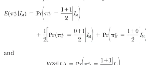
respec-E(q
ii⬘|IM)⫽ Pr
冢
qii⬘⫽1⫹1 2
兩
IM冣
tively, for the four states. Assume that the QTL is locatedbetween markerkandk⫹1 for 1ⱕkⱕM⫺1. What
we want is to calculate the probabilities of IBD states ⫹1
2
冤
Pr(q ii⬘⫽
0⫹1
2
兩
IM冣
⫹Pr冢
q ii⬘ ⫽
1⫹0 2
兩
IM冣冥
of the QTL conditional on the probabilities of IBDstates of all markers, i.e., Pr(q
ii⬘|1ii⬘, . . . ,Mii⬘). When
and the marker IBD states are not directly observed,
Pr(q
ii⬘|ii1⬘, . . . , iiM⬘) should be denoted by Pr(qii⬘|IM),
E(␦q
ii|IM)⫽Pr
冢
qii⬘ ⫽1⫹1 2
兩
IM冣
.whereIMmeans the marker information. From Bayes’
theorem, the probability of IBD states of QTL given the
expectations of the IBD matrices {⌸j} and {⌬j} can be jtakes the uniform distribution on the chromosome(s)
into consideration. The prior distributions of , 2 A, 2e,
used in the Bayesian analysis of QTL mapping. With
the conditional distribution method, the states of {⌸j} 2aj, and2djare assumed to be uniforms on predefined
and {⌬j} have to be sampled from their conditional distri- intervals, although other priors can be used. The lower
butions in the Bayesian procedure. In a maximum-likeli- and upper bounds for all variance components are
usu-hood (ML) analysis of IBD-based variance components, ally set to zero and the phenotypic variance present in
GesslerandXu(1996) discovered that the conditional the data, respectively.
distribution and expectation methods have virtually no A Markov chain Monte Carlo method is used to
gener-difference, but the conditional expectation method is ate the joint posterior distribution of all unknowns given
computationally much more efficient than the condi- in Equation 4. The idea of MCMC is to simulate a
ran-tional distribution method. Because of this, we use only dom walk in the space of the unknowns. The random
the conditional expectations in the proposed method, walk eventually converges to a stationary distribution.
i.e., replacing {⌸j} and {⌬j} by their conditional expecta- The stationary distribution represents the posterior
dis-tions. tribution of the unknowns. Various approaches have
been suggested to conduct the MCMC. The Metropolis-Hastings algorithm is a general term for a family of
BAYESIAN MAPPING FOR NORMALLY
Markov chain simulation methods that are useful for
DISTRIBUTED TRAITS
drawing samples from Bayesian posterior distributions The observables are the phenotypic valuesy⫽ {yi}ni⫽1, (Hastings 1970). The Metropolis algorithm and the
the covariate dataX, and the marker dataIM. The loca- Gibbs sampler are two commonly used special cases of
tions of markers on chromosomes are known a priori. the Metropolis-Hastings algorithm (Metropoliset al.
The list of unobservables contains the number of QTL 1953; Gemanand Geman1984). The reversible jump
l, the locations of QTL ⫽{j}lj⫽1, and the model effects MCMC is an extension of the Metropolis-Hastings
sam- ⫽(,2
a1, · · · , 2al, 2d1, · · · , d2l, 2A, 2e), where j pler, permitting posterior samples to be collected from
denotes the distance of thejth QTL from one end of posterior distributions with varying dimensions (Green
the chromosome in which the QTL resides. With the 1995). With our Bayesian analysis, the number of QTL
IBD-based variance component approach, the polygenic is treated as an unobservable, which naturally leads us
effects and the additive and dominance effects have to consider the problem within the general framework
been integrated out in the likelihood, and, therefore, of variable dimensional parameter estimation.
we do not have to generate them in the MCMC process. The proposed MCMC algorithm starts from an initial
From Bayes’ theorem, the joint posterior distribution point (l0, 0, 0) and proceeds to update each of the
of the parameters {l, , } given the observables and unknowns in turn. For an initial QTL position, we can
prior information is calculate the corresponding expectations of the IBD
matrices using the multipoint method. Updatingand
p(l,,|y)⬀p(y|l,,)p(l,,). (4)
is implemented using the Metropolis algorithm.
Up-Here, we have suppressed the notation for conditional dating the QTL number l requires a change in the
on the observed markers and covariate data. The first dimension of the model and thus needs a reversible
term in Equation 4 is the conditional distribution of jump step. More specifically, given the current state of
the phenotypic data given all unknowns, which is usually (l,,), we proceed with the MCMC as follows. called the likelihood, and has the following form:
Updating : All elements of are updated
simultane-ously. New proposals for the elements ofare
sam-f(y|l,,)⫽(2)⫺n/2|V|⫺1/2exp
冦
⫺12(y⫺X)
TV⫺1(y⫺X)
冧
.pled from the symmetric uniform densities around
(5) their previous values. The proposals are accepted
si-multaneously with probability The second term in Equation 4 is the joint prior
distribu-tion ofl,, and, the parameters of our interest.
Assum-min
1,
f(y|l,,*)
f(y|l,,)
, (7)
ing prior independence of the parameters, we can fac-torize the joint prior distribution p(l, , ) into the
where* represents the proposed. If the proposal following products:
is not accepted, then the state remains unchanged.
p(l,,)⫽p(l)p()p(2
A)p(2e)
兿
l
j⫽1
[p(j)p(2aj)p(
2
dj)]. Updatingandl: we adopt the method ofSillanpa¨a¨
andArjas(1998, 1999) to implement the reversible (6)
jump MCMC. They used three different types of moves: (1) modify the QTL locations when the
num-The prior distribution of the number of QTL, l, is
assumed to be truncated Poisson with mean l and a ber of QTL is unchanged; (2) add one new QTL to
the model; and (3) delete an existing QTL from the
predefined maximum numberL.When no information
other hand, ifl⫽L, the maximum number of QTL the variances are all accepted simultaneously; otherwise, the QTL number remains unchanged.
assigned a priori, we cannot add a QTL. When 0 ⬍
l ⬍ L, the different types of moves have proposal Whenpdhappens, we delete a QTL from the model,
each existing QTL being equally likely to be deleted. If
probabilities of pm ⫽ 1/3, pa ⫽ 1/3, or pd ⫽ 1/3
to remain unchanged, to add, or to delete a QTL, the j⬘th existing QTL is proposed to be deleted from
the model, the acceptance probability is respectively. Note that other values of pm,pa, and pd
can be used.
min
1,
|V*|⫺1/2exp{⫺1/2(y⫺ X)TV*⫺1(y⫺X)} |V|⫺1/2exp{⫺1/2(y⫺ X)TV⫺1(y⫺X)}
When the number of QTL remains unchanged, we modify the locations of the existing QTL. Following
Sillanpa¨a¨andArjas (1998, 1999), we do not fix the ⫻ l2pa
lpd
, (10)
order of QTL when updating the QTL locations.
Ele-ments ofare modified one at a time using the Metropo- where V*⫽ Rl
j⫽1⌸j2aj⫺ ⌸j⬘2aj⬘⫹R l
j⫽1⌬j2dj⫺ ⌬j⬘2dj⬘⫹
lis algorithm. For thejth QTL, a proposal*j is sampled A2
A⫹ I2e. If the proposal is accepted, we delete a QTL
from a uniform distribution on the interval [j⫺d,j⫹ from the model. Otherwise, the number of QTL remains
d], wheredis the tuning parameter. The expectations unchanged.
of the IBD matrices for new location *j, denoted by In Equations 9 and 10, the first term of the acceptance
⌸*j and⌬*j , are then formed according to the new posi- ratio is the likelihood ratio, and the second term
con-tion (*j ) and the marker information. The proposal is tains the prior ratio and the proposal ratio. Note that
accepted with probability here the Jacobian of the transformation is one because
adding one QTL or deleting one QTL does not influ-min
1,
|V*|⫺1/2exp{⫺ 1/2(y⫺X)TV*⫺1(y⫺X)} |V|⫺1/2exp{⫺ 1/2(y⫺X)TV⫺1(y⫺X)}
, ence the parameters of the other QTL.
(8) BAYESIAN MAPPING FOR BINARY TRAITS
where ⫺j means all elements of excluding the jth For a complex disease trait, the observed phenotype
element, is defined in a binary fashion,i.e.,wj⫽1 if an individual
is affected, andwj⫽0 otherwise. We propose an
underly-ing normal variableyjthat determines the binary
obser-V⫽
兺
l j⫽1
⌸j2aj⫹
兺
l j⫽1
⌬j2dj⫹A 2
A⫹I2e, vation. The link betweeny
jandwjis through a threshold
t,i.e., and
wj⫽
1 0
ifyj⬎t
ifyjⱕt
. (11)
V*⫽
兺
l j⬘⬆j
⌸j⬘2aj⬘⫹ ⌸*j2aj⫹
兺
l j⬘⬆j
⌬j⬘2dj⬘⫹ ⌬*j⬘2dj⫹A 2 A⫹I2e.
The liabilityyis nothing new but an unobservable quan-titative trait that can be described by Equation 1. The If the proposal is not accepted, the state remains
un-threshold model is overparameterized so that some con-changed, and the algorithm proceeds to update the
straints must be superimposed. As usual, we taket⫽0 location of the next QTL.
and2
e⫽1 (AlbertandChib1993). The expectation
Whenpahappens, we add a QTL to the model. The
of the liabilityyis the same as that of Equation 2, but location of the new QTL, l⫹1, is proposed from the
the variance-covariance matrix is uniform density on the chromosome(s) under
consider-ation. The expectations of the IBD matrices for the
Var(y)⫽ V⫽
兺
l
j⫽1
⌸j2aj⫹
兺
lj⫽1
⌬j2dj⫹A
2
A⫹ I. (12)
new QTL, denoted by⌸l⫹1and ⌬l⫹1, are then formed
according to the new position (l⫹1) and the marker
In the threshold model, the observables are the binary information. The additive and dominance variances of
phenotypic values w⫽ {wi}ni⫽1, the covariate data, and
the new QTL,2
al⫹1and2dl⫹1, are drawn from their priors. the marker data. The unobservables include the vector
The proposal is accepted with probability
of liabilityy⫽{yi}ni⫽1, the number of QTLl, the locations
of QTL ⫽{j}lj⫽1, and the model effects ⫽
min
1,
|V*|⫺1/2exp{⫺1/2(y⫺ X)TV*⫺1(y⫺ X)}
|V|⫺1/2exp{⫺1/2(y⫺ X)TV⫺1(y⫺X)} (,2a1, · · · ,2al,
2
d1, · · · ,2dl,
2 A).
The joint posterior distribution of the unobservables, {y,l,,}, after suppressing the notation for
condition-⫻ lpd
(l⫹ 1)2p a
, (9) ing on the marker data and the covariate data, can be
expressed as
where V* ⫽ Rl
j⫽1⌸j2aj ⫹ ⌸l⫹12al⫹1 ⫹ R
l
j⫽1⌬j2dj ⫹ ⌬l⫹1
p(y,l,,|w)⬀p(w|y,l,,)p(y|l,,)p(l,,), (13) 2
dl⫹1⫹A2A⫹I2e. If the proposal is accepted, we add
chromosome with a marker distance of 10 cM. Four
p(w|y,l,,)⫽
兿
n
i⫽1
p(wi|yi)⫽
兿
ni⫽1
{1(yi⬎0)1(wi ⫽1)
equally frequent alleles were simulated at each marker locus. Two QTL residing at positions 25 and 75 cM,
⫹ 1(yiⱕ0)1(wi⫽0)}, (14)
respectively, and 12 additional independent loci of
where 1(X 苸 A) is the indicator function, taking the equal effect (called polygene) were simulated for a
con-value of 1 ifXis contained inA, and 0 otherwise. Note tinuous phenotype. The dominance effect of the
poly-that p(w|y,l, , ) ⫽ p(w|y) because wis solely deter- gene was assumed to be absent. The variances of the
mined by y. The second term in Equation 13 is the first QTL were2
a1⫽ 2d1⫽0.6 and those of the second
conditional distribution of the liability given all other QTL were2
a2⫽ d22 ⫽0.4. The polygenic variance was
unknowns and has the same form as Equation 5. Finally, set at2
A⫽1.0. The normally distributed phenotype of
the last term in Equation 13 is the joint prior distribution each individual took the sum of an overall mean, values
ofl,, and. of QTL additive and dominance effects, polygenic
ef-From this joint posterior density, it can be seen that fect, and a residual error sampled from a standardized
the posterior distribution of the parametersl,, and normal distribution. In addition, we generated a binary
can be computed using the method for normally distrib- phenotype for each individual using the normally
dis-uted data if the liabilityyis known. To implement the tributed phenotypic value as the underlying liability.
MCMC algorithm for binary traits, therefore, we need The binary phenotype took 1 if the liability exceeded
to generate the liabilityy.Since it is difficult to simulate 0, and 0 otherwise. The overall mean was set to 0, which directly from the conditional distribution ofygivenw
led to 50% population incidence. We simulated 500 and other parameters, we use the method of the Gibbs
full-sib families, each with 6 siblings (a total of 3000
sampler (ChanandKuk 1997). The details are as
fol-individuals). For comparison, we analyzed both the nor-lows.
mal data and the binary data. No phenotypic values and Starting with some initial values y(0) ⫽ (y(0)
1 , · · · ,
marker linkage phases were recorded for all parents.
y(0)
n )T consistent in signs with the observed data w, we
In each of the MCMC analyses, we ran a single long proceed to generate y(t⫹1)⫽ (y(t⫹1)
1 , · · · ,y(nt⫹1))T,t ⫽ 0,
chain with 5⫻ 105 cycles of simulations. The first 200
1 · · · , sequentially in the following manner. Given the
samples were discarded and the chain was then thinned current state (y(t),l(t),(t),(t)) of all unknowns, we
simu-(we saved one iteration in every 50 cycles) to reduce late
serial correlation in the stored samples so that the total
y(t⫹1)
1 fromf(y1|y(t)2,y(t)3,· · · ,y(t)n,w;l(t),(t),(t)), number of samples kept in each analysis was 104.
.. The initial value for the QTL number was set at 1
.
and the corresponding initial location was given at the
y(t⫹1)
i fromf(yi|y(t1⫹1),y(t2⫹1), · · · ,y(ti⫺⫹11),y(t)i⫹1, · · · ,y(t)n,w;l(t),(t),(t)), 50-cM position of the chromosome. The prior Poisson
... mean of the number of QTL wasl⫽2 and the
maxi-mum number of QTL was L ⫽ 4. The starting values
y(t⫹1)
n fromf(yn|y1(t⫹1),y(t2⫹1), · · · ,y(tn⫺⫹11),w;l(t),(t),(t)).
were 0.0 for the overall mean, 1.0 for both the polygenic and residual variances, and 0.5 for both the additive To carry out the above simulations, we use the fact
and dominance variances of the QTL. The prior for the
f(yi|yj,j⬆i;w1, · · · ,wn;l,,)⫽f(yi|yj,j⬆i;wi;l,,).
overall mean was uniform over the range [⫺2.0, 2.0]. The priors for all variance components were chosen as Sincey⫽(y1, · · · ,yn)Thas aN(X,V) distribution, it
uniform on [0.0, 4.0], the right endpoint being equal follows thatf(yi|yj,j⬆i;l,,) is also normal with mean
to the true phenotypic variance of the liability. The
E(yi)⫹Cov(yi,y⫺i)(Var(y⫺i))⫺1(y⫺i⫺E(y⫺i))
prior for the QTL locations was uniform over the whole chromosome. The tuning parameter of the proposal and variance
distribution was set at 2 cM for QTL locations and 0.1 Var(yi)⫺ Cov(yi,y⫺i)(Var(y⫺i))⫺1Cov(y⫺i,yi),
for the overall mean and all variance components.
We used the QTL intensity function of Sillanpa¨a¨
wherey⫺i⫽(y1, · · ·,yi⫺1,yi⫹1, · · ·,yn)T. Thus,f(yi|yj,j⬆
andArjas(1998) to detect the number and locations
i;wi,l,, ) is a truncated (above 0 ifwi ⫽1; below 0
of QTL. In practice, we divided the chromosome into if wi ⫽ 0) normal distribution. Devroye’s algorithm is
then used to simulate a truncated normal variable (De- intervals of equal length (according to the Haldane
vroye 1986). distance) and then calculated the proportion of QTL
in each interval from the MCMC samples. The interval length was chosen to be 1 cM long. As done inStephens A SIMULATION STUDY
and Fisch (1998) and Sillanpa¨a¨ and Arjas (1999), the QTL variances were estimated from samples in
Design of the simulation experiment:The proposed
which QTL locations fall into the regions with suffi-method is illustrated in the analysis of a simulated
exam-ciently high estimated QTL intensities. ple. We simulated a single chromosome of length 100
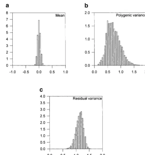
Figure2.—Approximate posterior distributions of the (a) overall mean, (b) polygenic variance, and (c) residual variance for normally distributed data.
and coincide with the simulated number of QTL. As expected, the posterior variance of QTL number for
Figure1.—Histograms of the posterior QTL intensity for the normal data is smaller than that for the binary data.
(a) normally distributed data and (b) binary data. The true Finally, the posterior modes of the QTL numbers over-number of QTL is two, located at positions 25 and 75 cM, lap with the true number of QTL in both data analyses. respectively.
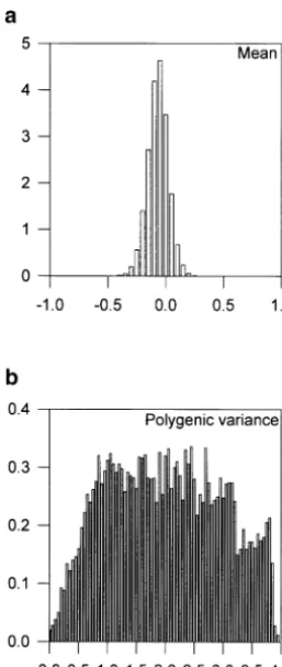
The posterior samples for the overall mean, the poly-genic variance, and the residual variance from the
nor-both the normal and the binary data are presented in mal data analysis, and those for the overall mean and
Figure 1. The QTL intensity graphs are concentrated the polygenic variance from the binary data analysis, are
around the true locations of the simulated QTL. One depicted in Figures 2 and 3, respectively. The posterior
peak of the posterior QTL intensity for the normal data means and standard errors of these parameters are given
is on [24, 25] and the other on [76, 77]. The correspond- in Table 3. From the figures and the table, it appears that
ing peaks for the binary data are on [23, 24] and [74, estimates of these parameters are close to the simulated
75], respectively. These results support quite strongly a values with small standard errors from the normal data.
model having two QTL in the chromosome. Comparing However, the polygenic variance is greatly overestimated
the shapes of the posterior QTL intensities for the bi- and the estimated standard error is large from the binary
nary and normal data analyses, we can see that binary data analysis although the mean is still estimated
accu-data analysis does lose some information, but the infor- rately.
mation retained is still sufficient to detect both QTL. The chromosome regions with sufficiently high
poste-The approximate posterior distributions on the QTL rior QTL intensity are given in Table 3. The posterior
number, obtained from the two types of data, are pre- samples, in which QTL locations fall into these regions,
sented in Table 2. The posterior expectations are essen- are used to estimate the QTL variances. Figures 4 and
5 depict such posterior samples for the QTL variances tially the same for the binary data and the normal data
TABLE 2
Inferred posterior distribution and posterior mean of the number of QTL
No. of QTL 0 1 2 3 4 Mean
errors are small. In the binary data analysis, however, the additive and dominance variances of the QTL are overestimated, and the standard errors are larger than those for the normal data.
The point estimates and the estimation errors of the QTL locations are also given in Table 3. For both types of data, the estimated QTL locations are very close to the corresponding true values. However, the standard errors are much larger for the binary data than those for the normal data.
For comparison, the simulated normal data set was
analyzed using the ML method (Xu and Atchley
1995). Figure 6 shows the likelihood profile along the chromosome when a single QTL was fitted to the model. We can see that the likelihood-ratio profile shows two peaks, the higher peak being at position 25 cM and the lower peak at position 76 cM, overlapping with the true locations of the two simulated QTL (at 25 and 75 cM, respectively). This result is consistent with results of the reversible jump MCMC analysis. The ML estimates of variances of the first QTL are ˆ2
a1⫽ 0.8253 andˆ2d1⫽
0.8900. The estimated variances of the second QTL are ˆ2
a2 ⫽ 0.7839 and ˆ2d2 ⫽ 0.5667. The ML estimates of
QTL variances are not so close to the corresponding true values as the estimated posterior means in the re-versible jump MCMC analysis.
Figure3.—Approximate posterior distributions of the (a) overall mean and (b) polygenic variance for binary data.
DISCUSSION
We have presented here a Bayesian procedure that from the normal data and the binary data analyses,
respectively. The posterior densities of QTL variances allows detection of multiple QTL for both normally
distributed and binary traits under IBD-based variance are concentrated around the corresponding true values
for both types of analyses, although the binary data component analysis. The proposed Bayesian procedure
is implemented via a reversible jump MCMC algorithm, analysis shows a wider distribution. More explicitly, we
calculated the means and the standard errors of the which enables moves to be made between models with
different numbers of QTL. We model complex binary posterior samples for the QTL variances (see Table 3).
For the normal data, the estimated posterior means of traits under the classical threshold model of quantitative
genetics (LynchandWalsh1998). The Bayes method
the additive and dominance variances of the QTL are
close to the simulated true values, and the standard of mapping QTL for binary traits is developed based
TABLE 3
The highest posterior QTL intensity intervals, Bayesian estimates of QTL locations, the additive and dominance variances of the QTL, and polygenic and residual variances
Sum of QTL Data Interval the QTL location
type (cM) intensity (cM) 2
aj
2
dj
2
A 2e
ⵑ18–29 0.9967 24.3013 0.7101 0.6886
Normal (1.1678) 0.028 (0.2480) (0.1994) 0.8696 1.1587
ⵑ72–84 0.9938 77.0253 (0.0559) 0.5701 0.3362 (0.2415) (0.1419) (2.2326) (0.1954) (0.1534)
ⵑ17–30 0.9405 23.2892 0.8443 1.0681
Binary (2.1665) ⫺0.0396 (0.4618) (0.5966) 1.5801
ⵑ64–86 0.9101 74.4903 (0.0816) 0.4493 0.7652 (0.7561) (4.7986) (0.3237) (0.5289)
Figure 4.—Approximate posterior distribu-tions of the QTL additive and dominance vari-ances for normally distributed data. (a) The first QTL additive variance determined from interval 18 cM toⵑ29 cM. (b) The first QTL dominance variance determined from interval 18 cM toⵑ29 cM. (c) The second QTL additive variance deter-mined from interval 72 cM toⵑ84 cM. (d) The second QTL dominance variance determined from interval 72 cM toⵑ84 cM.
on the idea of data augmentation. This treatment pro- chical model by treating the variance as the parameter
of interest. As a result, information about the number vides an easy way to generate the values of the normally
distributed latent variable, which in turn allows the use of alleles is not required, which has significantly
im-proved the robustness of the Bayes method. of Bayesian mapping for normally distributed traits. The
methodology can be easily generalized to multiple or- The IBD-based variance component approach of QTL
mapping is based on the proportion of alleles with iden-dered categorical traits (AlbertandChib 1993).
Bayesian mapping statistics have been well studied in tity-by-descent shared by relatives. Inference on IBD ma-trices does not need the information of marker linkage
the context of line-crossing experiments (Satagopan
andYandell1996;Satagopanet al.1996; Sillanpa¨a¨ phases. The IBD states of markers are calculated in advance and remain asa priorin the Bayesian procedure. andArjas1998, 1999; Stephens andFisch 1998), in
which the parameter of primary interest is the average With the proposed method, we can completely avoid the
complicated problem concerning sampling of additive effect of allelic substitution (the first moment). The
variance of the allelic substitution is given as a prior and dominance effects of QTL and marker and QTL
genotypes. The IBD-based variance component Bayes-and no further inference is made to the prior variance.
When applied to complex pedigrees, the Bayes method ian mapping is not limited to nuclear families. In the
simulation study, we used full-sib families to demon-can be formulated to fit different models of QTL
varia-tion (e.g., biallelic or normal QTL effects;Heath1997; strate the utility of the method solely for the purpose of simplicity. In theory, the Bayes method described in
UimariandHoeschele1997;Binket al.1998). In
con-trast to line-crossing experiments in which the number this article can be applied easily to extended or complex
pedigrees by using a general algorithm to compute the of alleles at the QTL is known exactly, in outbred
popu-lations, the number of alleles per locus is rarely known. IBD proportion shared by an arbitrary relative pair. Such
a general algorithm has been given by Almasy and
In most cases, we can assume two alleles in a relatively
homogeneous population, as made byHeath (1997) Blangero (1998). For large and complex pedigrees,
however, the computational burden may be prohibitive, andUimariandHoeschele(1997). As a consequence,
one must also estimate the allelic frequency to infer the due to the need for computation of the
variance-covari-ance matrixVand its inverse. genetic variance via ˆ2
a ⫽ 2pˆ(1 ⫺ pˆ)aˆ2. Although the
biallelic model may be proper in most situations, it can In the simulation study, we put two QTL on a single
chromosome and 12 independent loci on other unspeci-potentially fail if the actual number of polymorphic
alleles is not two. The IBD-based variance component fied chromosomes as a “polygene.” Our model always
hierar-Figure 5.—Approximate posterior distribu-tions of the QTL additive and dominance vari-ances for binary data. (a) The first QTL additive variance determined from interval 17 cM toⵑ30 cM. (b) The first QTL dominance variance deter-mined from interval 17 cM toⵑ30 cM. (c) The second QTL additive variance determined from interval 64 cM toⵑ86 cM. (d) The second QTL dominance variance determined from interval 64 cM toⵑ86 cM.
The polygenic variance varies depending on the model somes) in the model instead of being absorbed into
the polygenic term. The other strategy is to map QTL effects fitted. Without this polygenic term, variances due
to QTL on unmarked chromosomes or chromosome simultaneously for all chromosomes. In the latter
situa-tion, if the marker map is sufficiently dense, the poly-regions will join the residual variance. A large residual
variance will reduce the power of QTL detection. In genic term can be ignored because eventually all QTL
will be identified and their effects will be explicitly esti-practice, we can take one of three strategies for QTL
mapping. One strategy is to analyze one chromosome mated. These three mapping strategies may produce
similar results. at a time. Marker information on other chromosomes
can be completely ignored. In this case, variances of The reversible jump MCMC sampler performed well
for the simulated normally distributed and binary data. QTL on other chromosomes will be collected by the
polygene (not the residual). The second strategy is to A plot of the changes in the number of QTL against
the number of iterations for the binary data used in the include the previously identified QTL (at other
chromo-simulation study is presented in Figure 7. It shows that the reversible jump MCMC algorithm mixes well over the number of QTL. A similar plot was obtained for the normally distributed data. We detected no influence of initial values of unknowns on the mixing of the MCMC sampler. For example, with the simulated data, starting
with l0 ⫽ 4, the QTL number lquickly dropped to 1
after several hundred iterations and subsequently
be-haved the same as starting with l0 ⫽ 1. The mixing
behavior of the number of QTL is greatly affected by the prior distributions for QTL additive and dominance variances (StephensandFisch1998). As expected, in-creasing the upper bounds of the uniform prior distribu-tions has the general effect of decreasing the acceptance rates of adding a new QTL to the model and deleting
Figure6.—Likelihood-ratio profile of ML mapping from
a QTL from the model. With the upper boundc⫽4.0
normally distributed data. There are two QTL, located at
able. However, our treatment simplifies the MCMC algo-rithm and does not result in a significant reduction in efficiency particularly when the marker map is dense. It has been shown that, conditional on the IBD states of a marker locus, the IBD matrices of a QTL on one side of the marker are not correlated to those of a QTL
on the other side (Xu andAtchley1995). In case of
two tightly linked QTL in the same marker interval, the IBD matrices of these two QTL are always highly correlated no matter what methods are used to infer them. The correlation between two QTL can be com-pletely eliminated by the assumption that any marker interval includes at most one QTL. Under this assump-tion, the acceptance probabilities for adding one QTL
and deleting one QTL should be modified (Stephens
Figure7.—The trace of the number of QTL for the binary
andFisch1998).
data, for 104saved samples after burn-in.
Finally, Bayesian statistics have the inherent flexibility introduced by their incorporation of multiple levels of
rates for both adding and deleting steps wereⵑ0.4% randomness and the resultant ability to combine
infor-for both the simulated normally distributed and binary mation from different sources. Therefore, the Bayesian
data. These acceptance rates were similar to those in approach could be extended to allow more complicated
Sillanpa¨a¨andArjas(1998). The acceptance rates for models under more complicated data structures, e.g.,
both adding and deleting steps increased to 3% when the epistatic model. When a new QTL is proposed, its
the upper bound was set atc⫽1.0. By comparison, the interactive effects with all existing QTL should be
pro-acceptance proportions for updating QTL locations and posed and, if accepted, the epistatic effects should be
model effectswere found to be rather high in general included in the model. A QTL is finally added to the
and wereⵑ80% for the simulated data. model if at least one effect caused by the QTL is
ac-A major implementation issue in MCMC is to deter- cepted. This will involve additional reversible jumps on
mine the effective sample sizes. This issue is related to the dimension of the model even if the number of QTL
the assessment of convergence of the chain, the serial remains the same.
correlation between the samples, and the burn-in
pe-We thank Dr. Damian Gessler for his helpful comments on the
riod. For a single long chain, one can examine time manuscript. We also thank two anonymous reviewers for their critical series graphs of a simulated sequence to judge whether comments on an earlier version of the manuscript. This research was supported by the National Institutes of Health Grant GM55321 and the
the chain is sufficiently long (Geyer 1992).
Subsam-United States Department of Agriculture National Research Initiative
pling the chain at regular intervals is a common practice
Competitive Grants Program 97-35205-5075 to S.X.
to reduce the serial correlation between the samples. With the reversible jump MCMC algorithm, however, it is difficult to calculate autocorrelation of the MCMC
samples for all parameters because the dimension keeps LITERATURE CITED
changing from one cycle to another. When the dimen- Albert, J. H.,andS. Chib,1993 Bayesian analysis of binary and sion changes, the identities of the QTL also change. polychotomous response data. J. Am. Stat. Assoc.88:669–679.
Almasy, L.,andJ. Blangero,1998 Multipoint quantitative-trait
link-The parameters in one cycle of the iteration may be
age analysis in general pedigrees. Am. J. Hum. Genet.62:1198–
different from those in the next cycle of iteration. In 1211.
our simulation studies, therefore, we empirically deter- Amos, C. I., 1994 Robust variance-components approach for as-sessing genetic linkage in pedigrees. Am. J. Hum. Genet. 54:
mined the lengths of the chain, subsampling intervals
535–543.
and the burn-in period. We used the plots of the changes Bink, M. G. A. M., L. L. G. JanssandR. L. Quaas,1998 Mapping in the number of QTL against the number of iterations a polyallelic quantitative trait locus using simulated tempering. Proceedings of the 6th World Congress on Genetics Applied to
to determine an approximate burn-in period. The length
Livestock Production Science, Armidale, Australia, Vol. 26, pp.
of subsampling intervals was chosen to eliminate
obvi-277–280.
ous changing trends for all parameters. Chan, J. S. K.,andA. C. Kuk,1997 Maximum likelihood estimation
for probit-linear mixed models with correlated random effects.
We only use marker information to infer the IBD
Biometrics88:86–97.
matrices of QTL and allow multiple QTL located in the
Devroye, T.,1986 Non-uniform Random Variable Generation.
Springer-same marker interval in the proposed method. Alterna- Verlag, New York.
Duggirala, R., J. T. Williams, S. Williams-BlangeroandJ. Blan-tively, we can infer the IBD matrices of a QTL
consid-gero,1997 A variance component approach to dichotomous
ered by utilizing the IBD information of all markers
trait linkage analysis using a threshold model. Genet. Epidemiol.
and other existing QTL in the same chromosome and 14:987–992.
Fulker, D. W., andL. R. Cardon, 1994 A sib-pair approach to
accept-interval mapping of quantitative trait loci. Am. J. Hum. Genet. Rao, S.,andS. Xu,1998 Mapping quantitative trait loci for ordered categorical traits in four-way crosses. Heredity81:214–224.
54:1092–1103.
Rebai, A.,1997 Comparison of methods for regression interval map-Fulker, D. W., S. S. ChernyandL. R. Cardon,1995 Multipoint
ping in QTL analysis with non-normal traits. Genet. Res.69:
interval mapping of quantitative trait loci, using sib pairs. Am. J.
69–74. Hum. Genet.56:1224–1233.
Satagopan, J. M.,andB. S. Yandell,1996 Estimating the number of Geman, S.,andD. Geman,1984 Stochastic relaxation, Gibbs
distribu-quantitative trait loci via Bayesian model determination. Special tions, and the Bayesian restoration of images. IEEE Trans. Pattern
Contributed Paper Session on Genetic Analysis of Quantitative Anal. Machine Intell.6:721–741.
Traits and Complex Diseases, Biometric Section, Statistical Meet-Gessler, D. D. G.,andS. Xu,1996 Using the expectation or the
ing, Chicago, IL. distribution of identity-by-descent for mapping quantitative trait
Satagopan, J. M., B. S. Yandell, M. A. NewtonandT. G. Osborn, loci under the random model. Am. J. Hum. Genet.59:1382–1390.
1996 A Bayesian approach to detect quantitative trait loci using Geyer, C. J.,1992 Practical Markov chain Monte Carlo. Stat. Sci.7:
Markov chain Monte Carlo. Genetics144:805–816. 473–511.
Schork, N. J.,1993 Extended multipoint identity-by-descent analysis Goldgar, D. E.,1990 Multipoint analysis of human quantitative
of human quantitative traits: efficiency, power, and modeling genetic variation. Am. J. Hum. Genet.47:957–967.
considerations. Am. J. Hum. Genet.53:1306–1319. Green, P. J.,1995 Reversible jump Markov chain Monte Carlo
com-Sillanpa¨a¨, M. J.,andE. Arjas,1998 Bayesian mapping of multiple putation and Bayesian model determination. Biometrika82:711– quantitative trait loci from incomplete inbred line cross data.
732. Genetics148:1373–1388.
Grignola, F. E., I. HoescheleandB. Tier,1996 Mapping
quantita-Sillanpa¨a¨, M. J.,andE. Arjas,1999 Bayesian mapping of multiple tive trait loci via residual maximum likelihood: I. Methodology. quantitative trait loci from incomplete outbred offspring data.
Genet. Sel. Evol.28:479–490. Genetics151:1605–1619.
Hackett, C. A.,andJ. I. Weller,1995 Genetic mapping of quantita- Stephens, D. A.,andR. D. Fisch,1998 Bayesian analysis of quantita-tive trait loci for traits with ordinal distributions. Biometrics51: tive trait locus data using reversible jump Markov chain Monte
1252–1263. Carlo. Biometrics54:1334–1347.
Haley, C. S.,andS. A. Knott,1992 A simple regression method Uimari, P.,andI. Hoeschele,1997 Mapping linked quantitative for mapping quantitative trait loci in line crosses using flanking trait loci using Bayesian analysis and Markov chain Monte Carlo
markers. Heredity69:315–324. algorithms. Genetics146:735–743.
Hastings, W. K.,1970 Monte Carlo sampling methods using Markov Visscher, P. M., C. S. HaleyandS. A. Knott,1996 Mapping QTL chains and their applications. Biometrika57:97–109. for binary traits in backcross and F2populations. Genet. Res.68:
55–63. Heath, S. C.,1997 Markov chain Monte Carlo segregation and
Xu, S.,andW. R. Atchley,1995 A random model approach to linkage analysis of oligogenic models. Am. J. Hum. Genet.61:
interval mapping of quantitative trait loci. Genetics141:1189– 748–760.
1197. Jansen, R. C.,1993 Interval mapping of multiple quantitative trait
Xu, S.,andW. R. Atchley,1996 Mapping quantitative trait loci loci. Genetics135:205–211.
for complex binary diseases using line crosses. Genetics 143:
Kao, C. H., Z-B. ZengandR. D. Teasdale,1999 Multiple interval
1417–1424. mapping for quantitative trait loci. Genetics152:1203–1216.
Xu, S.,andD. D. G. Gessler,1998 Multipoint genetic mapping of Kruglyak, L.,andE. S. Lander,1995 Complete multipoint
sib-quantitative trait loci using a variable number of sibs per family. pair analysis of qualitative and quantitative traits. Am. J. Hum.
Genet. Res.71:73–83. Genet.57:439–454.
Yi, N.,andS. Xu,1999a Mapping quantitative trait loci for complex Lynch, M.,andB. Walsh,1998 Genetics and Analysis of Quantitative
binary traits in outbred populations. Heredity82:668–676.
Traits.Sinauer Associates, Sunderland, MA.
Yi, N.,andS. Xu,1999b A random model approach to mapping Mendell, N. R.,andR. C. Elston,1974 Multifactorial qualitative quantitative trait loci for complex binary traits in outbred
popula-traits: genetic analysis and prediction of recurrence risks. Biomet- tions. Genetics153:1029–1040.
rics30:41–57. Zeng, Z-B.,1994 Precision mapping of quantitative trait loci. Genet-Metropolis, N., A. W. Rosenbluth, M. N. Rosenbluth, A. H. ics136:1457–1468.
TellerandE. Teller,1953 Equation of state calculations by