ABSTRACT
NAGAPPAN, NACHIAPPAN. A Software Testing and Reliability Early Warning (STREW) Metric Suite. (Under the direction of Dr. Laurie A. Williams.)
The demand for quality in software applications has grown, and awareness of software testing-related issues plays an important role towards that. Unfortunately in industrial practice, information on software field quality of a product tends to become available too late in the software lifecycle to affordably guide corrective actions. An important step towards remediation of this problem lies in the ability to provide an early estimation of post-release field quality.
A Software Testing and Reliability Early Warning (STREW)
Metric Suite
By
Nachiappan Nagappan
A DISSERTATION SUBMITTED TO THE GRADUATE FACULTY OF NORTH CAROLINA STATE UNIVERSITY
IN PARTIAL FULFILLMENT OF THE REQUIREMENTS FOR THE DEGREE OF
DOCTOR OF PHILOSOPHY
COMPUTER SCIENCE
Raleigh, NC
2005
Approved by:
Dr. Christopher G. Healey Dr. Jason A. Osborne
Dr. Mladen A. Vouk Dr. Laurie A. Williams
Om
To Appa and Amma….+
+
Biography
Acknowledgements
This thesis would not have been possible without the help of several people. It is impossible to acknowledge everyone I have worked with in the 22 years of my academic life. If I have missed you, I apologize for the mistake but want you to know that you are gratefully remembered.
First and foremost, I would like to thank Laurie for being a fantastic advisor. I met Laurie for the first time on a Wednesday, Nov 14 2001 at 11.00 AM. That was our first meeting. From that time on till today it’s been a pleasure to work with her. I appreciate her patience, encouragement and support through these years. She has always watched out for me, helped me with all my problems and has always been open in her views. Her comments/feedback is something I will miss. Thanks, Laurie.
Dr. Vouk has been a truly inspiring mentor. I have always been amazed by his ability to think of several possible solutions to a problem whenever I have got stuck. His experience and insight have greatly influenced my work. I hope this work meets the high standards set by him.
My other committee members Dr. Jason Osborne and Dr. Chris Healey have been supportive of my work through these years. Dr. Osborne took the trouble of explaining statistics to a computer science major in addition to spending long hours explaining various statistical modeling techniques and packages and the significance of interpreting the results. My understanding of “the why and how of statistics” has been greatly influenced by him. Dr. Healey has been supportive of my work and has showed a lot of interest in my future goals and plans after graduation. I sincerely appreciate all his help.
used in this dissertation, the developers in the industrial software organization, and the students of CSC 326 in Fall 2003 are gratefully acknowledged for their contribution towards this thesis.
My thanks are also due to Martin for working with me on GERT and my friends at NC State Guru, CK, Pradeep (both), Yogi, Dinesh, Prabhakar and Karthikeyan who have made my stay at NCSU very enjoyable.
On an organizational level, I would like to thank the Department of Computer Science, (especially Margery Page and Vilma Berg) and North Carolina State University, for proving an excellent environment for a student 8801 miles (14164 km) from home.
Finally last but in no way least, Chidambaram Arunachalam, Annan and Akka for keeping me sane, taking care of me and feeding me on a regular basis. Without you people, my stay here would not have been possible, and I would not have graduated…. and my brother for being the motivation for me to finish up before he did….
TABLE OF CONTENTS
Page No.
LIST OF TABLES ………..……… ix
LIST OF FIGURES ………..………….. xi
1. INTRODUCTION ………..……… 1
2. BACKGROUND ………..……….. 4
2.1 SOFTWARE RELIABILITY ……… 4
2.2 SOFTWARE TESTING ……… 6
2.2.1 SOFTWARE TESTING CLASSIFICATIONS ………... 6
2.2.2 AUTOMATED SOFTWARE TESTING EXAMPLE USING JUNIT ……… 8 2.3 SOFTWARE METRICS ………... 11
2.3.1 TEST METRICS ……….. 13
2.3.1.1 PRODUCT METRICS (DEFECT/ERROR/FAULT METRICS) ……… 14
2.3.1.2 PROCESS METRICS ………... 15
2.3.2 HALSTEAD SOFTWARE SCIENCE ………. 16
2.3.3 CYCLOMATIC COMPLEXITY ………. 17
2.3.4 FUNCTION-POINT ANALYSIS ……… 18
2.3.5 HENRY-KAFURA STRUCTURE METRIC ……….. 19
2.3.6 OBJECT-ORIENTED METRICS ……… 20
2.3.6.1 CK METRICS ……….. 20
2.3.6.2 MOOD METRIC SUITE ………. 21
2.4 INDUSTRIAL METRIC PROGRAMS ………... 21
2.4.1 MOTOROLA ………... 21
2.4.2 HEWLETT-PACKARD ……….. 22
3. RELATED RESEARCH ………..……….. 24
3.1 PRIOR RELATED WORK ………... 24
3.2 SOFTWARE RELIABILITY MODELS ……….. 28
4. STREW METRIC SUITE ………..………… 37
5. POST-RELEASE FIELD QUALITY ESTIMATION ……….... 46
5.1 FEASIBILITY STUDY ………. 47
5.2 MODEL BUILDING ………. 49
5.3 RESULTS EVALUATION TECHNIQUES ………. 51
5.4 ACADEMIC CASE STUDY ……… 52
5.4.1. DESCRIPTION ………... 52
5.4.2 MODEL BUILDING ……… 53
5.4.3 RANDOM DATA SPLITTING ………... 54
5.5 OPEN SOURCE CASE STUDIES ………... 55
5.5.1. DESCRIPTION ………... 56
5.5.2 MODEL BUILDING ……… 58
5.5.3 RANDOM DATA SPLITTING ………... 59
5.6 INDUSTRIAL CASE STUDY ……….. 65
5.6.1. DESCRIPTION ………... 65
5.6.2 POST-RELEASE FIELD QUALITY PREDICTION ……….. 66
6. TEST QUALITY FEEDBACK ……….……… 69
6.1 BUILDING TEST QUALITY FEEDBACK STANDARDS ……… 70
6.2 EVALUATION OF TEST QUALITY FEEDBACK STANDARDS …... 73
6.3 CASE STUDIES ……… 73
6.3.1 ACADEMIC CASE STUDY ……….... 74
6.3.2 OPEN SOURCE CASE STUDY ……….. 75
6.3.3 STRUCTURED INDUSTRIAL CASE STUDY ……….. 77
6.4 STATISTICAL ANALYSIS OF TEST QUALITY FEEDBACK... 79
6.5 QUALITATIVE ANALYSIS ……… 82
7. RETROSPECTIVE STREW METRIC ANALYSIS ……….. 88
8. CONCLUSIONS AND FUTURE WORK ……….…………... 98
REFERENCES ………..………. 101
APPENDIX A - DATA SETS ………..……….. 110
APPENDIX B – TOOL SUPPORT ……….……….. 112
LIST OF TABLES
Page No.
Table 3.1: Legend for classification of software reliability models ………. 30
Table 3.2: Software Reliability model classification ……… 31
Table 4.1: Corresponding source and test code ……… 38
Table 4.2: STREW metrics and collection and computation instructions ………... 40
Table 5.1: Pearson correlation and statistical significance results between the ratios and the reliability estimate ……….. 49
Table 5.2: Prediction evaluation results ……… 54
Table 5.3: Component matrix for PCA transformation ……… 59
Table 5.4: AAE and ARE values ……….. 64
Table 5.5: Sensitivity evaluation for PCA models ……… 65
Table 5.6: Industrial project sizes ………. 65
Table 5.7: Project characteristics ……….. 66
Table 6.1: Color coded feedback standards ……….. 71
Table 6.2: STREW metric color coded feedback explanation ……….. 71
Table 6.3: Desired correlation results with the color-coded feedback ……….. 73
Table 6.4: Academic case study – correlation results ………... 75
Table 6.5: Open source case study – correlation results ………... 77
Table 6.6: Industrial project data description ……… 78
Table 6.7: Industrial case study – correlation results ……… 79
Table 6.8: Summary correlation results of test quality feedback ……….. 80
Table 6.9: Comparative modeling results ………. 81
Table 6.10: Simple linear regression coefficients ………. 81
Table 6.11: Test quality feedback standards – open source case study ……… 82
Table 6.12: Release 1 STREW metrics feedback ………. 83
Table 6.13: Release 2 STREW metrics feedback ………. 83
Table 6.14: Release 3 STREW metrics feedback ………. 84
Table 6.15: Release 4 STREW metrics feedback ………. 84
Table 6.16: Release 5 STREW metrics feedback ………. 85
Table 6.18: Type 1 and Type II errors ……….. 86
Table 6.19: Type I, Type II errors for case studies ………... 86
Table 7.1: Correlation Matrix – Academic Projects ………. 92
Table 7.2: Correlation Matrix – Open Source projects ………. 93
Table A.1: Academic case study data set ……….. 110
Table A.2: Open source case study data set ……….. 111
Table B.1: Statistics for the past 10 months ……….. 114
Table B.1: Statistics for All Time (courtesy sourceforge.net) ………. 115
Table C.1: One-Sample Kolmogorov-Smirnov Test – Academic Projects ……….. 116
Table C.2: One-Sample Kolmogorov-Smirnov Test – 27 Open Source Projects …. 116 Table C.3: Correlation matrix with individual project metrics – Academic ………. 121
LIST OF FIGURES
Page No.
Figure 2.1: Testing Techniques ………. 7
Figure 2.2: Example Java Source program ………... 8
Figure 2.3: Example Java Test program ………... 9
Figure 2.4: JUnit output screen shot ………. 11
Figure 2.5: Software metrics classification ………... 13
Figure 4.1: Corresponding source and test classes ………... 38
Figure 4.2: STREW metric revision process ……… 42
Figure 4.3: Example cyclomatic complexity computation ………... 43
Figure 4.4: Sample assertion and test case measurement example ……….. 44
Figure 4.5: CBO, DIT and WMC measurement example ……… 44
Figure 5.1: Empirical case studies ……… 47
Figure 5.2: Academic projects size ………... 53
Figure 5.3: Normal probability plot for model fitting ………... 54
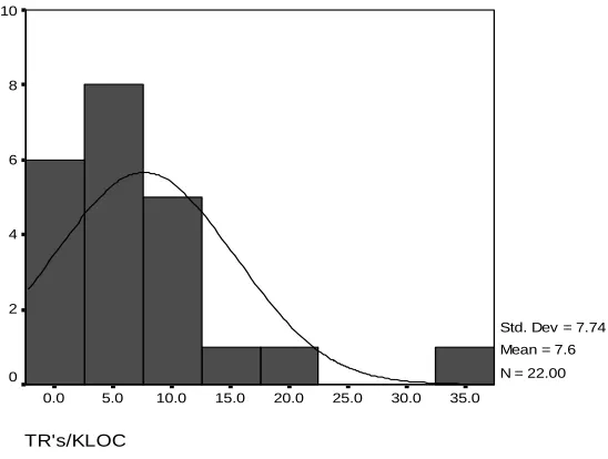
Figure 5.4: Histogram of TRs/KLOC in academic projects ……….………… 55
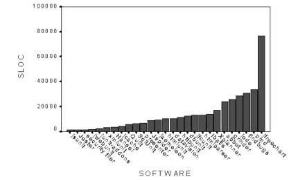
Figure 5.5: Open source project sizes ………... 57
Figure 5.6: Model fitting results for PCA ………. 58
Figure 5.7: Random data split – model building and evaluation results …………... 59
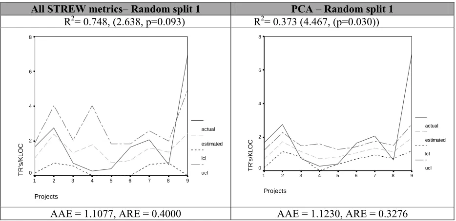
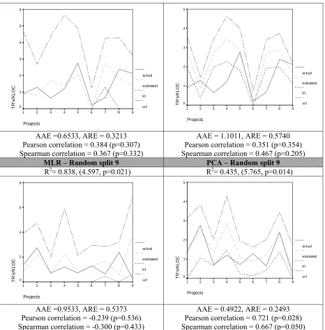
Figure 5.8: Prediction plots with all the STREW metrics ………. 66
Figure 5.9: Prediction plots with PCA ……….. 67
Figure 6.1: Color coded feedbacks-Academic case study ……… 74
Figure 6.2: Project size across three years ……… 76
Figure 6.3: Color coded feedbacks for open source case study ……… 76
Figure 6.4: Color coded feedbacks for structured industrial case study …………... 78
Figure 7.1: Scatterplots of TRs Vs. Size ………... 89
Figure 7.2 Scatterplots of TRs/KLOC Vs. Size ……… 89
Figure 7.3: 3-D plots of Asserts/KLOC vs. Test Cases/KLOC vs. TRs/KLOC …... 90
Figure 7.4: 3-D plots of Asserts vs. Test Cases vs. TRs ………... 91
Table 7.6: Scatter plots of STREW metrics with TRs/KLOC ……….. 94
Figure B.1: GERT snap shot ………. 112
Figure B.2: Usage Statistics (courtesy sourceforge.net) ……….…….. 114
Figure C.1: Normality plot of regression residuals – Academic case study ….…… 117
Figure C.2: Normality plot of regression residuals –Open source case study …….. 117
Figure C.3: Scree plot ………... 118
Figure C.4: Component plot ………. 119
Figure C.5: Scree plot ………... 119
CHAPTER 1
INTRODUCTION
Software engineering is the application of a systematic, disciplined, quantifiable approach to the
development, operation, and maintenance of software; that is, the application of engineering to
software[43]. A more mathematical definition of Software Engineering was presented by Boehm in
the classic Software Engineering Economics book [10] ,
Software engineering is the application of science and mathematics by which the
capabilities of computer equipment are made useful to man via computer programs,
procedures, and associated documentation. [10]
Software Engineering activities include: Managing, Costing, Planning, Modeling, Analyzing,
Specifying, Designing, Implementing, Testing and Maintaining of software [33].
In industry, estimates of software field quality are often available too late in the software lifecycle
to affordably guide corrective actions to the quality of the software. As a result, true field quality
cannot be measured before a product has been completed and delivered to an internal or external
customer. Because this information is available late in the software lifecycle, corrective actions tend
to be expensive [10]. Software developers can benefit from an early warning regarding the quality of
their product.
In our research, we formulate this early warning from a collection of internal testing metrics that
obtained from users. A TR [60] is a customer-reported problem whereby the software system does not
behave as the customer expects. An internal metric, such as cylomatic complexity [58], is a measure
derived from the product itself [44]. An external measure is a measure of a product derived from the
external assessment of the behavior of the system [44]. For example, the number of failures found in
test is an external measure.
The ISO/IEC standard [44] states that “internal metrics are of little value unless there is evidence
that they are related to some externally visible quality.” Internal metrics have been shown to be
useful as early indicators of externally-visible product quality [3] when they are related (in a
statistically significant and stable way) to the field quality/reliability of the product. The validation of
such internal metrics requires a convincing demonstration that (1) the metric measures what it
purports to measure and (2) the metric is associated with an important external metric, such as field
reliability, maintainability, or fault-proneness[29].
Our research objective is to construct and validate a set of easy-to-measure in-process metrics
that can be used as an early indication of an external measure of post-release field quality and
provides meaningful feedback on the thoroughness of a testing effort. To this end, we have created a
metric suite we call the Software Testing and Reliability Early Warning metric suite for Java
(STREW-J) [69-71]. Software reliability is defined as the probability that the software will work
without failure under specified conditions and for a specified period of time [64].
The STREW metrics are used to build a regression model to estimate the post-release field
quality using the metric TRs/KLOC. The estimation of post release field quality via the STREW
metric suite is applicable for development teams that write extensive automated test cases, such as is
done in the Extreme Programming [8] software development methodology. The STREW method is
not applicable for script-based automated testing because, as will be discussed, the metrics are
primarily based upon the object-oriented (O-O) programming paradigm. Teams develop a history of
the value of the STREW metrics from comparable projects with acceptable levels of field quality.
elements and the TRs/KLOC. In this dissertation, we present empirical results of an academic
feasibility study (22 projects), a case study of open source projects (27 projects), and an industrial
case study (five projects) designed to build and validate the STREW model.
The rest of this thesis is organized as follows. Chapter 2 provides the background introduction to
software reliability, software testing, software metrics, and industrial metric programs. Chapter 3
outlines the prior research work related to the estimation of fault density and fault-proneness, and
Chapter 4 presents the STREW metric suite. Chapters 5 and 6 provide the evaluation of the STREW
metric suite in terms of estimating the post-release field quality and providing test quality feedback.
Chapter 7 presents a retrospective analysis of the STREW metric suite, and Chapter 8 discusses the
CHAPTER 2
BACKGROUND
This section provides an introduction to the four main areas related to this proposal: software
reliability, software testing, software metrics, and industrial metric programs.
2.1 SOFTWARE RELIABILITY
Software reliability is defined as the probability that the software will work without failure under
specified conditions and for a specified period of time [64]. A number of software reliability models
are available. They range from the simple Nelson model [73] to more sophisticated hyper-geometric
coverage-based models [45], to component-based models, and object-oriented models [3]. Several
reliability models use Markov Chain techniques [95]. Other models are based on the use of an
operational profile, i.e., a set of software operations and their probabilities of occurrence [64]. These
operational profiles are used to identify potentially-critical operational areas in the software to signal
a need to increase the testing effort in those areas. A large group of software reliability growth models
are described by Non-Homogenous Poisson Processes (NHPP) [98]. This group includes Musa [66]
and the Goel-Okumoto [35] models.
In many test-centric methodologies, developers strive to pass all the automated tests that are
written, and there are no measurable faults. Even if there are failures, these failures might not be an
Instead, “no failure” estimation models, as described in [26, 28, 59], may be more appropriate for use
with such methodologies.
Software reliability models can be classified broadly into seven categories [97]:
• Markov models: A model belongs to this class if its probabilistic assumption of the
failure process is essentially a Markov process, i.e. a birth-death process. In these
models each state of the software has a transition probability associated with it that
governs the operational criteria of the software.
• Non-homogeneous Poisson process (NHPP) models: A model is classified as a
NHPP model if the main assumption is that the failure process is described by a NHPP.
The main characteristic of this type of model is that there is a mean value function which
is defined as the expected number of failures up to a given time.
• Bayesian process: In a Bayesian process model, some interesting information about
the software to be studied is available before the testing starts, such as inherent fault
density and defect information of previous releases. This information can be used in
combination with the collected test data to make a more accurate estimation and
prediction about the reliability.
• Statistical data analysis methods: Different statistical models and methods are
applied for the analysis of software failure data. Some of these models are the time series
model, proportional hazards model, and regression models.
• Input-domain based models: These models do not make any dynamic assumption
about the failure processes. All possible input and output domains of the software are
constructed and, based on the results of the testing, the faults in mapping between the
input and output domains are identified, i.e. for a particular value in the input domain if
• Seeding and tagging models: These models utilize the statistical capture-recapture
technique that involves the artificial seeding of faults. The assessment of the testing is
based upon the number of seeded faults that remain in the software at the conclusion of
the testing effort.
• Software metrics models: Software reliability metrics which are measures of the
software complexity can be used to estimate the number of software faults remaining in
the software.
2.2 SOFTWARE TESTING
Software testing is a verification and validation (or V&V) software practice and is considered to
be a software quality assurance practice. Software testing can be use to answer two main questions
[10],
• Verification: Are we building the product right?
• Validation: Are we building the right product?
2.2.1 SOFTWARE TESTING CLASSIFICATIONS
As shown in Figure 2.1, testing activities can be classified as black box or white box. Black box
testing [43], (also called functional testing) is testing that ignores the internal mechanism of a system
or component and focuses solely on the outputs generated in response to selected inputs and
execution conditions. Black box testing is used to simulate the customer behavior and focuses on
input/output. White box testing [43], (also called structural testing) is testing that takes into account
Figure 2.1: Testing Techniques
There are several levels of testing that should be done on a large software system. These levels are
explained below [43].
1. Unit Testing: Testing of individual hardware or software units or groups of related units[43]. It is done at a very low structural level. The primary objectives of unit testing
are to (1) verify the code against the component, i.e. to see if the code does what the
component is expected to do with respect to the overall system; (2) execute all new and
changed code to ensure all branches are executed in all directions, (3) check for the
correctness of logic and data paths; and (4) exercise all error messages, return codes and
response options [48].
2. Integration testing: Testing in which software components, hardware components, or both are combined and tested to evaluate the interaction between them. Integration testing
involves uses both black and white box testing techniques[43].
3. Functional and System testing: Using black box testing techniques, testing conducted on a complete, integrated system to evaluate the system's compliance with its specified
requirements[43].
4. Acceptance testing: (1) Formal testing conducted to determine whether or not a system satisfies its acceptance criteria and to enable the customer to determine whether or not to
Software Testing
accept the system. (2) Formal testing conducted to enable a user, customer, or other
authorized entity to determine whether to accept a system or component[43].
5.
Regression testing. Selective retesting of a system or component to verify thatmodifications have not caused unintended effects and that the system or component still
complies with its specified requirements[43].
2.2.2 AUTOMATED SOFTWARE TESTING EXAMPLE USING JUNIT
As this dissertation deals with leveraging the software testing effort for estimating post-release
field quality, we present an example of the xUnit1 type of software testing that our post-release field
quality is based upon. Note the symmetries between the source and test code. This example involves
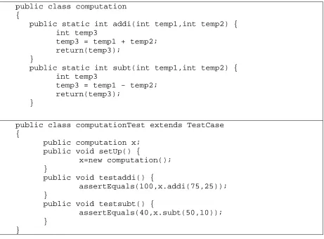
a Java program to add, subtract, multiply and divide two numbers, as shown in Figure 2.2.
Source Program
//computation.java
//author-Nachiappan Nagappan
import java.io.*; import java.lang.*;
public class computation {
//Add two numbers
public static int addi(int temp1,int temp2) {
int temp3;
temp3=temp1+temp2;
return(temp3);
}
//Subtract two numbers
public static int subt(int temp1,int temp2) {
int temp3;
temp3=temp1-temp2;
return(temp3);
}
//Multiply two numbers
public static int mult(int temp1,int temp2) {
int temp3;
temp3=temp1*temp2;
return(temp3);
}
//Divide two integers
public static int divi(int temp1,int temp2) {
int temp3;
temp3=temp1/temp2;
return(temp3);
}
public static void main(String args[])throws IOException {
int x;
computation nachi=new computation(); }
} //End of Program
Figure 2.2: Example Java Source program
There are four methods that form the core of the source program, addi(), subt(), mult() and divi()
which perform the operations of addition, subtraction, multiplication and division. The corresponding
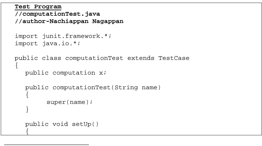
automated testing program written in JUnit2 is given in Figure 2.3. This test program exercises the
source program to check if the operations are correct based on specific test cases (e.g. testaddi() in
Figure 2.3 to check if two integers are added correctly).
Test Program
//computationTest.java
//author-Nachiappan Nagappan
import junit.framework.*; import java.io.*;
public class computationTest extends TestCase {
public computation x;
public computationTest(String name) {
super(name);
}
public void setUp() {
x=new computation(); }
//Test addi() method of computation.java
public void testaddi() {
x=new computation();
assertEquals(100,x.addi(75,25));
}
//Test subt() method of computation.java
public void testsubt() {
x=new computation();
assertEquals(50,x.subt(75,25));
}
//Test mult() method of computation.java
public void testmult() {
x=new computation();
assertEquals(1875,x.mult(75,25));
}
//Test divi() method of computation.java
public void testdivi() {
x=new computation();
assertEquals(3,x.divi(75,25));
}
public static void main(String[] args) {
}
} //End of Program
Figure 2.3: Example Java Test program
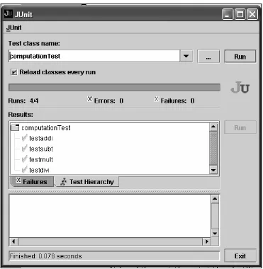
Upon execution of the above test program, all the four mathematical operations are tested and the
JUnit output is produced, as shown in Figure 2.4. Figure 2.4 shows that four of four test cases pass
Figure 2.4: JUnit output screen shot
2.3 SOFTWARE METRICS
We present in this section a discussion on software metrics as we use in-process testing metrics in
our dissertation research. The term software metrics explains many activities, all of which involve
some degree of software measurement [33]:
• Cost and effort estimation
• Productivity measures and models
• Data collection
• Reliability models
• Performance evaluation and models
• Structural and complexity metrics
• Capability-maturity assessment
• Management by metrics
• Evaluation of methods and tools.
Since there is virtually an infinite number of possible software metrics, developers must have
some criteria for choosing which metrics to apply for a particular project. Ideally, a metric should
possess the following characteristics [77]:
• Simple. The definition and use of the metric is simple;
• Objective. If different people perform the measurement, they will give similar values.
Objective metrics allow for consistency and prevents individual bias;
• Easily collected. The cost and effort to obtain the measure is reasonable;
• Robust. The metric is insensitive to irrelevant changes, allowing for useful comparison;
and
• Valid. A valid metric measures what it is supposed to measure, promoting trustworthiness
of the measure.
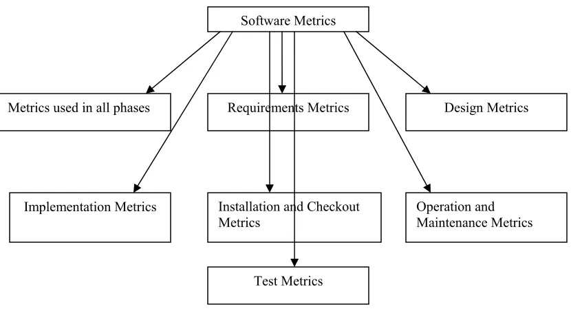
Software metrics may be broadly classified into seven categories [77] as shown in Figure 2.5. The
seven categories represent the seven different phases of software engineering from which metrics can
Figure 2.5: Software Metrics Classification
The STREW metric suite is comprised of metrics from both the source and test code. The
following discussion presents a broad overview of the popular software metric measures. The metrics
range from product, process metrics to metric measurement paradigms like the Halstead metrics,
cyclomatic complexity, and function points.
2.3.1 TEST METRICS
We shall concentrate on a study of the test metrics [77] because in our work, we leverage the
testing effort to assess the quality of the testing effort and to predict post-release field quality based
on previous empirical data. Test metrics may be of two types [77],
1. Metrics related to test results or the quality of the product being tested.
2. Metrics used to assess the effectiveness of the testing process.
In this dissertation, we will be focusing on metrics of the second category. Further, we also provide
an overview of some of the product (metrics obtained from the software) and process (metrics
obtained from the software process employed in the development cycle) metrics that are commonly
used.
Software Metrics
Installation and Checkout Metrics
Implementation Metrics
Design Metrics Requirements Metrics
Metrics used in all phases
Operation and Maintenance Metrics
2.3.1.1 PRODUCT METRICS
(Defect/Error/Fault Metrics)
• Primitive defect/error/fault metrics. These are very simple, easy to collect metrics that are
represented in terms of bar, line graphs and using histograms.
• Number of faults detected in each module.
• Number of requirements, design, and coding faults found during unit and integration testing.
• Number of errors by type (e.g. number of logical errors, number of computation errors,
number of interface errors etc.)
• Number of errors by cause or origin
• Number of errors by severity (number of critical errors, number of major errors, number of
cosmetic errors).
• Fault Density (FD): Number of faults/size in one thousand lines of code (KLOC)
o FD may also be weighed in using the severity of errors as shown in Equation 2.1.
FD (Weighted) = W1 S/N+W2 A/N+W3 M/N (2.1)
W1,W2 ,W3 – Weights assigned.(User dependant)
N- Number of faults
S-Number of severe faults
A-Number of average severity faults
M-Number of minor faults
• Defect age: Defect age is the time between when a defect is introduced and when it is fixed.
The average defect age of a product is computed using the summation of the individual defect
ages for all the defects as shown in Equation 2.2.
defect age= Σ∀(Phase detected – phase introduced)/ Number of defects (2.2)
• Defect response time: This measure is the time between when a defect is detected to when it
• Defect Cost: The cost of a defect is the sum of the cost to analyze the defect, the cost to fix it,
and the cost of failures already incurred due to the defect.
• Defect removal efficiency (DRE): The defect removal efficiency is the percentage of defects
that have been removed during a process, computed via Equation 2.3.
DRE = Number of defects removed/Number of defects at the start of the process * 100% (2.3)
2.3.1.2 PROCESS METRICS
Test case metrics
• Total number of planned white/black box test cases run to completion.
• Number of planned integration tests run to completion
• Number of unplanned test cases required during the test phase.
Coverage metrics
• Statement coverage
• Branch coverage
• Path coverage
• Data flow coverage
• Test coverage
Failure metrics
• Mean time to failure (MTTF): This is the mean time for the next failure i.e. (i+1)th failure
giventhe failure times of the previous i failures. This metric is a basic parameter required
by most software reliability models.
• Failure rate: This is used to indicate the growth in the software reliability as a function of
test time and is usually used with reliability models. Failure rate requires the observed
time between failures at a given severity level and the number of failures in a given
shown in Equation 2.4, is obtained from the cumulative probability distribution (F(t)) of
the time until the next failure, using a software reliability estimation model.
o The failure rate, λ(t)= -1/R(t) [dR(t)]/dt where R(t)=1-F(t) (2.4)
• Cumulative failure profile. Uses a graphical technique to predict reliability to estimate
additional testing time needed to reach an acceptable reliability level and to identify
modules and subsystems that require additional testing.
Some of the more commonly used software metric(s)/suites are discussed below. These models
provide an introduction to current trends in software metrics measurement.
2.3.2 HALSTEAD SOFTWARE SCIENCE
Halstead [37] proposes the measurement of a software system that is obtained by breaking down
and arranging a finite number of program “tokens,” which are basic syntactic units distinguished by a
compiler. Halstead’s measurement takes into account the number of distinct operators and operands
that appear in a program; the total number of operator occurrences; and the total number of operand
occurrences to calculate several program characteristics. These characteristics are program length
(total number of operator and operand occurrences), volume (number of bits required to specify a
program), vocabulary (total count of distinct operator and operand count), level (a measure of
software complexity), and program effort.
Using the above metrics, Halstead designed a set of equations that express several of the program
characteristics.
Vocabulary (n): n = n1 + n2 (2.5)
Length (N): N= N1 + N2 (2.6)
= n1 log2(n1) + n2 log2(n2)
Volume (V): V= N log2 (n) (2.7)
= N log2 (n1 + n2)
= (2/n1) * (n2/N2)
Difficulty (D) = 1/L (2.9)
Effort (E): E= V/L (2.10)
Faults (B): = V/S* (2.11)
Where:
• n1- The number of distinct operators that appear in a program
• n2- The number of distinct operands that appear in a program
• N1- The total number of operator occurrences
• N2- The total number of operator occurrences
• V* is the volume represented by the built in function performing the task of the entire
program
• S* is the mean number of mental discriminations (decisions) between errors (S* is 3000
according to Halstead).
Halstead’s metrics has been subject to criticism in several aspects, such as methodology,
derivations of equations, human memory models [48]. Empirical support is lacking in several areas of
the Halstead measures. The Halstead metrics are static metrics that ignore variations in fault rates
observed in software products and among modules. However, Halstead’s work was instrumental in
making metrics an issue among computer scientists as it was the first formal investigation of software
metrics. [48]
2.3.3 CYCLOMATIC COMPLEXITY
McCabe designed cyclomatic complexity [58] as a measure of the programs testability and
understandability. Both testability and understandability impact maintainability [48]. Cyclomatic
complexity is adapted from the classical graph theoretical cyclomatic number to suit software science
and can be defined as the number of linearly-independent paths through a program. Cyclomatic
The formula used to compute the complexity metric is shown in Equation 2.12.
M = V(G) = e-n+2p (2.12)
Where, V(G) = cyclomatic complexity of G
e = number of edges
n = number of nodes
p=number of unconnected parts of the graph.
To have good testability and maintainability, McCabe recommended that no program module
should have a cyclomatic complexity greater than 10. Because it is based on decisions and branches,
this complexity metric is consistent with the logic pattern of design and programming, which appeals
to software professionals. Many experts recommend the use McCabe’s cyclomatic complexity to
ensure adequate test coverage, and the use of McCabe’s cyclomatic measure has been gaining
acceptance by practitioners [48].
2.3.4 FUNCTION-POINT ANALYSIS
Function point analysis [2] is an approach for assessing the size of a piece of software based on
the functionality provided. Function points are obtained by the analysis of a requirements
specification document to identify the different functions that the system is to perform. The functions
are classified into different types and are given weightings according to the relative complexity of the
function type [85].
For example, the unadjusted function point count ‘ufc’ for a specification is given by [85]
Equation 2.13:
ufc = 4*i+5*o+4*e+7*p+10*f (2.13)
where, i = number of external input types
o = number of external output types
e = is the number of enquiries
p = is the number of external files (program interfaces)
(This is a simplified equation from [85] to illustrate ufc)
Further, Albrecht suggests that a total of 14 complexity metric factors be taken into account for
calculating the technical complexity factor (tcf) [85]. The 14 factors are data communications,
distributed data processing, performance, heavily-used configuration, transaction rate, on-line data
entry, end-user efficiency, on-line update, complex processing, reusability, installation ease, operation
ease, multiple sites, facilitate change. Each factor is scored between zero (no influence) and five (very
strong influence). The tcf is calculated as shown in Equation 2.13:
tcf = 0.65 + 0.01 *
∑
i
DI (2.13)
,where DIi is the degree of influence of the ith technical complexity factor.
Thus, the tcf will range from 0.65 to 1.65. For a simple system with no data communications the
value will tend towards 0.65. A distributed system dealing with high transaction volumes and
characterized by complex processing have a tcf of approximately 1.35. Combining the technical
complexity factor and the unadjusted function point count, we obtain the adjusted function point
count (fp) as in Equation 2.14:
fp = ufc*tcf (2.14)
The function point is usually used as a predictor of the development effort, although its inverse is
often also used as a productivity index. Also, for example, once the function points of an organization
are calibrated, they have been found to explain 75% of the variation in program size in a study of 15
commercial software systems [49].
2.3.5 HENRY-KAFURA STRUCTURE METRIC
Structure metrics take into account the interactions between modules in a product or system and
quantify such interactions. The information-flow metric defined by Henry and Kafura [41], uses
fan-in (a count of the number of modules that call a given module) and fan-out (a count of the number of
modules that are called by a given module) to calculate a complexity metric.
Cp = (fan-in * fan-out)2 (2.15)
In general, modules with a large fan-in are relatively small and simple. In contrast, modules that are
large and complex have a small fan-in. Thus, components with a large fan-in and large fan-out may
indicate poor design. Such modules have to be decomposed correctly.
2.3.6 OBJECT-ORIENTED METRICS
In recent years, object-oriented (O-O) programming has gained importance, and new suites of
metrics that exploit the O-O properties are becoming popular. Two popular O-O metric suites are
presented below.
2.3.6.1 CK METRICS
The CK metric suite proposed by Chidamber-Kemerer (CK) [17]identifies six O-O metrics:
• Weighted Methods per class (WMC). the weighted sum of all the methods defined in a
class;
• Coupling Between Objects (CBO): the number of other classes with which a class is
coupled;
• Depth of Inheritance Tree (DIT): the length of the longest inheritance path in a given
class;
• Number of Children (NOC): the count of the number of children (classes) that each class
has;
• Response for a class (RFC): the count of the number of methods that are invoked due to
the initiation of an object of a particular class; and
• Lack of Cohesion of Methods (LCOM): is a count of the number of method pairs whose
similarity is zero and minus the count of method pairs whose similarity in not zero.
Several studies have been performed assessing the effectiveness of the CK Metrics in addressing
2.3.6.2 MOOD METRIC SUITE
The MOOD [15] O-O metric suite consists of the following O-O Metrics:-
• Method Hiding Factor (MHF): the number of visible methods;
• Attribute Hiding Factor (AHF): the number of visible attributes;
• Method Inheritance Factor (MIF): the ratio of the sum of inherited methods to the total
number of methods.
• Attribute Inheritance Factor (AIF): the ratio of, the sum of inherited attributes to the total
number of attributes.
• Polymorphism Factor (PF): the degree of method overriding in the class inheritance tree.
PF equals the number of actual method overrides divided by the maximum number of
possible method overrides.
• Coupling Factor: the actual number of couplings among classes in relation to the
maximum number of possible couplings.
2.4 INDUSTRIAL METRIC PROGRAMS
This section provides an insight into the popular metric programs employed in three popular
industrial organizations (Motorola, Hewlett-Packard, and IBM) to present an overview of the types of
metrics that are measured in commercial software development organizations.
2.4.1 MOTOROLA
Motorola’s software metrics program [21] follows the Goal/Question/Metric paradigm [6]. The
goals and measurement areas identified by the Motorola Quality Policy for Software Development
(QPSD) are listed below [48]:
Goals
• Goal 1: Improve project planning
• Goal 2: Increase Defect containment
• Goal 4: Decrease software defect density
• Goal 5: Improve customer service
• Goal 6: Reduce the cost of nonconformance
• Goal 7: Increase software productivity
Measurement areas:
• Delivered defects and delivered defects per size
• Total effectiveness throughout the process
• Adherence to schedule
• Estimation accuracy
• Number of open customer problems
• Time that problems remain open
• Cost of nonconformance
• Software reliability
2.4.2 HEWLETT-PACKARD
Hewlett- Packard’s software metrics program [36] uses several metrics and ratios to assess product
quality. A subset of these metrics is given below [48]:
• Average fixed defects/working day
• Average engineering hours/fixed defect
• Average reported defects/working day
• Branches covered/ Total branches
• Defects/thousands of non-commented source statements
• Defects/Lines of Documentation not included in program source code
• Defects/Testing time
• non-commented source statements /engineering month
• Engineering months/Total Engineering months
2.4.3 IBM ROCHESTER
For the software community within IBM, a set of standard 5-UP software quality metrics is
defined by the IBM corporate software measurement council. The 5-UP metrics include the following
[48]:
• Overall customer satisfaction
• Post release defect rate for three years
• Customer problem calls
• Fix response time
• Number of defective fixes
IBM Rochester in addition to the above 5-UP metrics uses several other in-process metrics, such
as phase effectiveness (for each phase of effectiveness and test); inspection coverage; effort; defect
rates; in-process inspection escape rate; compilation of failures and build/integration defects; weekly
defect arrivals and backlog during testing; defect severity; defect cause; reliability; models for post
CHAPTER 3
RELATED RESEARCH
In this chapter, we present the related research work in two sections. Section 3.1 is a discussion of
prior related studies done with software metrics, and Section 3.2 investigates the applicability of
popular software reliability models within our research context.
3.1 PRIOR RELATED WORK
The higher the failure-proneness of the software, logically the lower the reliability and the quality
of the software produced, and vice-versa. Software fault-proneness is defined as the probability of
the presence of faults in the software [23]. Failure-proneness is the probability that a particular
software element will fail in operation. Using operational profiling information, it is possible to relate
failure-proneness and fault-proneness of a product. Research on fault-proneness has focused on two
areas: (1) the definition of metrics to capture software complexity and testing thoroughness and (2)
the identification of and experimentation with models that relate software metrics to fault-proneness
[24]. While software fault-proneness can be measured before deployment (i.e. the count of faults per
structural unit such as faults per line of code), failure-proneness cannot be directly measured on
software before deployment [31]. Fault-proneness can be estimated based on directly-measurable
software attributes if associations can be established between these attributes and the system
Structural O-O measurements, such as those defined in the CK [17] and MOOD [15] O-O metric
suites, are being used to evaluate and predict the quality of software [39]. Structural
object-orientation (O-O) measurements, such as those in the Chidamber-Kemerer (C-K) O-O metric suite
[17], have been used to evaluate and predict fault-proneness [3, 13, 14]. The CK metric suite
consists of six metrics: weighted methods per class (WMC), coupling between objects (CBO), depth
of inheritance tree (DIT), number of children (NOC), response for a class (RFC) and lack of cohesion
among methods (LCOM). These metrics can be a useful early internal indicator of externally-visible
product quality in terms of fault-proneness [3, 86, 88].
In software systems, the actual measurable product quality (e.g., failure rate) that is derived from
the behavior of the system usually cannot be measured until too late in the life-cycle to effect an
affordable corrective action. In general, a multi-phase approach must be taken collecting the various
metrics of these suites at different stages, since different metrics will be visible at different
development phases [92, 93].
Basili et al. [3] studied the fault-proneness in a class on eight student projects. It was observed
that the WMC, CBO, DIT, NOC and RFC were correlated with defects while the LCOM was not
correlated with defects. Further, Briand et al. [14] performed an industrial case study and observed
the CBO, RFC, LCOM to be associated with the fault-proneness of a class. A similar study done by
Briand et al. [13] on eight student projects showed that classes with a higher WMC, CBO, DIT and
RFC were more fault prone while classes with more children (NOC) were less fault prone (LCOM
was not associated with the defects). Tang et al. [88] studied three real time systems for testing and
maintenance defects. Higher WMC and RFC were found to be associated with fault-proneness. El
Emam et al. [30] studied the effect of project size on fault-proneness by using a large
telecommunications application. Size was found to confound the effect of all the metrics on
fault-proneness. In addition to this, Chidamber et al.[17] analyzed project productivity, rework, and design
effort of three financial services applications. High CBO and low LCOM were associated with lower
empirical evidence that supports the theoretical validity of the use of these internal metrics [3, 13] as
predictors of fault-proneness. The consistency of these findings varies with the programming
language [86]. Therefore, the metrics are still open to criticism. [19]
The relationship between product quality and process capability [82] and maturity has been
recognized as a major issue in software engineering based on the premise that improvements in
process will lead to higher quality products. The process capability is defined as the ability of a
process to address the issue of stability, as defined and evaluated by trend or change. Such a
relationship between product quality and process capability should manifest itself via meaningful
metrics that would exhibit trends and other characteristics that would be indicative of the stability of
the process. Using the Space Shuttle software Schneidewind reports an assessment of long term
metrics, such as MTTF, total failures per KLOC change in code (churn), total test time normalized by
KLOC change in code, remaining failures normalized by KLOC, change in code, and predicted time
to next failure to be indicative of the stability of the software process with respect to process
capability [82].
Several techniques have been used for the analysis of software quality (errors3) with respect to
program metrics. Linear regression analysis techniques have been used to relate quality factors, such
as defect density and reliability, to software metrics. These regression models are built using the best
fit among all the data available and can be used to predict the software quality factors accordingly
using the current values of the metrics for programs that are being analyzed[63]. Discriminant
analysis, a statistical technique that is used to categorize programs into groups (high, moderate, low
quality) based on the programs metric values, are also used as a tool for the detection of fault-prone
programs. Munson et al. demonstrated the efficacy of discriminant analysis by using the technique
called data-splitting. From a total of 390 programs, 260 were randomly-selected and were used to
3 (1) The difference between a computed, observed, or measured value and the true, specified, or theoretically
build the discriminant model. The remaining 130 programs were used to test the efficacy of the
model to classify programs according to software faults. Discriminant analysis has been shown to
work well for programs with a low error rate, but the linear regression models shows greater promise
for use with programs with a high potential for faults[62]. Further, using Binary Discriminant Factors
(BDFs) makes fewer mistakes in classifying software that is of low quality than in the case with linear
vectors of metrics [83].
Also, optimized set reduction (OSR) techniques and logistic regression techniques are used for
modeling risk and fault data. OSR techniques attempts to determine which subsets of observations
from historical data provide the best characterization of the programs being assessed. Each of these
optimal subsets is characterized by a set of predicates (a pattern), which can be applied to classify
new programs. OSR is sometimes better than a logistic regression analysis for multivariate empirical
modeling since pattern-based classification is more accurate than logistic regression equations [12].
Further, logistic regression models can be built that relate software measures and software fault
proneness for classes of homogenous software products [24]. Also, multivariate models can be built
with logistic regression where Principal Component Analysis (PCA) is used on the of metrics to
model the data [25]. Denaro et al. calculated 38 different software metrics for the open source Apache
1.3 and Apache 2.0 projects. Using PCA, they selected a subset of consisting of nine of these metrics
was found to explained 95% of the total variance. Using combinations of these nine metrics, logistic
regression models were built using the data from the Apache 1.3 project and verified against the
Apache 2.0 project [25]. We believe that a judicious use of early metrics, in conjunction with an
understanding of the software process can be a powerful tool in guiding the development of good
3.2 SOFTWARE RELIABILITY MODELS
For our research, we must select an appropriate estimation model which can take as input a
quantification of the automated testing effort. We considered a large number of published software
reliability estimation models. Early in the research, the use of an operational profile-based reliability
model was determined to be impractical for use with development teams that write extensive
automated test cases (i.e. employ automated testing methods (ATM)). ATM is the existence of a dual
hierarchy of executable source and test code that work in parallel, for example Java source programs
and Junit test programs. An example for this is provided in Chapter 4. The infeasibility of using
operational profiles was determined based upon the results of three case studies [68] carried out in
industrial locations, John Deere, Rolemodel Software, and Nortel. We had initially assumed there
was a correspondence between the customer requirements and the developers automated acceptance
test cases. This assumption came from the idea that, during the requirements elicitation process, the
developers and customers would create the requirements and then the developers write acceptance
tests that dealt specifically with that certain requirement. In this way, developers could prove to the
customer that a given requirement was completed by demonstrating that its acceptance test(s) passed.
Thus, we expected that there would be a correspondence between a requirements and its acceptance
test case(s) for the life of the product.
However, we found that developers tend to aggregate a minimal set of acceptance test cases, each
used to satisfy several of the customer’s requirements. For example, the developers could have an
acceptance test that tested a certain core capability of the program. After this test passes, this core
capability is deemed to be implemented. As a result, developers consider that they do not need to
keep that test in its current form any more, and they build upon this test case to demonstrate more
complex behavior of another requirement. As more functionality is added to the system, developers
for multiple requirements. Therefore, developing a mapping between requirements and acceptance
test cases was shown to not be practical.
The main problems with using an operational profile-based model were identified as:
(1) Developers would need to change their automated acceptance testing habits to eliminate
the reuse and alteration of test cases;
(2) It is almost impossible to tie together the customer requirements and developer’s
acceptance test cases as developers tend to aggregate acceptance test cases to satisfy
several of the customer’s requirements; and
(3) The requirements of a software system continuously evolve across a release and this
evolution requires the developers to constantly reassign and recalculate the operation
profiles of the acceptance and unit tests which involves tremendous overhead. The
developers in the case study would not consider such a change to their current agile
methodology.
This lead us to the conclusion that the use of an operational profile model may not be feasible and
our approach would have to focus on using a non-operational profile models [78] for estimation of
reliability.
We set out to base our estimation model upon existing reliability models. The results of the first
round of the model selection effort are summarized in Tables 3.1 and 3.2. The selection criterion that
was used is based on the following constraints:
1. An operational profile-based model is impractical for our work.
2. In an ATM, all the test cases pass and there are no measurable failures.
3. Time is not monitored during testing/running of test cases in ATM. Therefore, defects
per unit time of operation cannot be measured.
4. No information regarding the inherent defect density (i.e. the number of defects
remaining in the software) is available. The inherent defect density is generally obtained
like Functional Verification test (FVT) at the end of which a testing group would say, for
example that there are 5 defects/KLOC based on their testing principle.
Twenty-two existing models were analyzed for identifying their fit within our problem domain.
We classified these models into one of four categories: Candidate, Bad Model Fit, Bad Data Fit, and
Overall Poor Fit. Table 3.1 shows the legend for the classification of the models. For example, if a
model could be used with an ATM but needed data that was not available with an ATM, it was
classified as a “Bad Data Fit.” In the data applicability criterion we assess if the product data
(metrics) available from software systems can be used for the modeling purposes. Information
regarding assumptions about the remaining number of failures in the system or process information
about the software system which is not easy to measure forms a crucial part in classifying models as a
bad data fit.
Table 3.1: Legend for Classification of Software Reliability Models
Applicability to data available
Applicability to ATMs Model Classification
Yes Yes Candidate
Yes No Bad Model Fit
No Yes Bad Data Fit
No No Overall Poor Fit
The classification of the twenty-two software reliability models according to the above
classification is shown in Table 3.2. The far majority of the models have a Bad Model Fit because
they require information about the previous failures (or require failures to occur) which would make
the model inapplicable if the system had no failures. Ultimately, we used a empirical metric model
Table 3.2: Software Reliability model classification Candidate Models
Empirical Metric Models, Lipow [55]: Several metrics are collected from previously-successful software programs. Using these metrics, a regression equation is framed that is
used to estimate the reliability of similar programs. If data from similar previous projects is
available for calibration, this model can be used.
Regression Models[63]: A linear regression analysis is investigated between the faults and certain selected metrics and parameters, such as field project quality. Works well with all
the data available.
Zero Failure Model [59]: The zero failure model determines the reliability when there are no failures, as shown below. To use the Zero-Failure model, we must identify a meaningful
long term failure rate denoted by Θ and that N random tests have established an upper
confidence bound (1-α) that Θ is below some level θ [38]. The relationship between these
factors is given by 1- (1-θ)N <= α [89]. Easy applicability but does not work for large
systems; Used in our feasibility studies.
Bad Model Fit
Nelson Model[73]: This is a very simplistic model based on the number of test failures. R = 1-(ň/n).
where
• ň - number of failures during testing.
• n-total number of testing runs.
• R is the system reliability.
If no failures are available, the reliability becomes 100% which might always not be the case
Table 3.2 (continued)
Fault seeding models, Schick and Wolvertone [80] and Duran and Wiorkowski [27]: The model requires fault injection whereby faults are intentionally injected into the software by
the developer. The testing effort is evaluated based upon how many of these injected defects
are surfaced during testing. Using the number of injected defects remaining, an estimate on
the reliability based on the quality of the testing effort is computed. Infeasible because it
requires process changes needing developers to do fault injection.
Hypergeometric Distribution, Tahoma et al. [87]: The number of faults experienced by test instance t(i) is required. Using the number of faults experienced by each test instance,
the overall system reliability can be determined. But in ATM there are no measurable
failures and usually the number of failures in each testing instance is not measured or
tracked. With ATMs, all the test cases pass, and there are no faults/failures to analyze.
Fault Spreading Model, Wohlin and Korner [96]: Requires number of faults at a level (or testing cycle/stage). The number of faults at each level is utilized to make predictions about
untested areas of the software. With ATMs, all the test cases pass, and there are no
faults/failures to analyze.
Fault Complexity Model, Nakogawa and Hanata [72]: Ranking of faults according to complexity. Based on the number of faults in each complexity level, the reliability of the
system is estimated based on the current complexity level (high, moderate, low) of the
software. With ATMs, all the test cases pass, and there are no faults/failures to analyze.
Littlewood-Verall Model [56]: Requires a scale parameter, Ψ(i), that is used for describing the quality of the test, and is a monotonically-increasing function. Failures are exponentially
distributed with a parameter assumed to have a prior Gamma distribution. With ATMs, all
Table 3.2: (continued)
Jelinski-Moranda (JM) Model [46]: In the JM model, the initial number of software faults in unknown but fixed (i.e. non-increasing), and the times between the failures are
exponentially distributed random quantities. Using this information, the JM model is
modeled as a Markov process model. But in ATMs, there are no failures, and the times of the
failure are also not measured.
Bayesian Formulation of the JM model, Langberg-Singpurwalla [54]: This models the parameters in the JM model as random variables. Poor fit for the same explanation as for the
JM model.
Bayesian Model for fault free probability, Thompson and Chelson [90]: This model delas
with the probability of fault-free software. Reliability at time t, R(t/λ,p) = (1-p) + pe-λt, where
λ is given by a prior gamma distribution and p (probability that software is not fault-free) is
given by an beta distribution. Using these parameters, a Bayesian model is constructed to
estimate the reliability. This model cannot be used because lamda and p cannot be fixed
without prior information of the defect density. Also, the defects may not follow a Beta
Distribution and with ATMs, all the test cases pass, and there are no faults/failures to
analyze.
Bayesian Model using a Geometric Distribution, Liu [57]: In this model let, Xi be the number of test cases at the ith debugging instanceat which the first failure will occur. Using
this value, the number of failures remaining at the current debugging instance can be
determined.
Table 3.2: (continued)
Goel-Okumoto Model [35]: The mean value function of the failures at time t is given by, m(t)=a(1-e-bt) where in time t the cumulative failures are observed; a and b are parameters
defined from the collected failure data. With ATMs, all the test cases pass, and there are no
faults/failures to analyze.
S-shaped model,Yamada, Ohba et.al. [98] : m(t)= a[1-(1+bt)e-bt] Where,
• a is the number of faults detected
• b is the failure detection rate
With ATMs, all the test cases pass, and there are no faults/failures to analyze.
Basic Execution Time Model [65] : λ(τ) – fK[N0-µ(τ)] Where,
• f and K are parameters related to the testing phase, initial fault density (N0)
• µ(τ)-faults corrected after τ amount of testing
• λ(τ) is failure rate function at the execution time τ.
This model cannot be applied as we do not have the initial fault density, and the failure rate
function at execution time τ with the ATMs.
Logarithmic Poisson Model [67] : Based on the Basic Execution Time Model (above).
λ(τ)= λ0 e-Φµ(τ) Where,
• λ0 is the initial failure intensity
• Φ is the failure intensity decay parameter.
Table 3.2: (continued)
Duane Model also known as the Weibull Process Model [26] : m(t)= (t/α)β
The two parameters α and β are based on failure data, m(t) is the mean value function of the
failures at time t. With ATMs, all the test cases pass, and there are no faults/failures to
analyze.
Markov Models, Shantikumar [84] and Whittaker and Poore [75]: Requires transition probabilities from state to state. Using this information a stochastic model is created and
analyzed for stability. This is primarily because there can be a very large number of states in
a large software program. Determining the states and the transition between the states
would require a process change that is likely to be unwelcome to developers that
utilize a ATM.
Fourier Series Model, Crow and Singpurwalla [20]: Fault clustering and time series analysis form a basis of this model. Using time series analysis, the model predicts how
clustered the faults will be at a given point in time. The ‘time’ parameter is not available as
in ATM only the number of tests (or testing runs) can be measured. With ATMs, all the test
cases pass, and there are no faults/failures to analyze.
Bad Data Fit
Input Domain-based Models, Bastani and Ramamoorthy [7] and Weiss and Weyuker [94]: Input domain is denoted by I of program P. I is mapped to output space O. If there is a fault
in mapping, then that mapping is identified as a potential fault to be rectified. Applicable,
but infeasible to map the domains are there can be a very large number of possibilities in a
Table 3.2 (continued)
Overall Poor Fit
Halstead Metrics [37], modified by Schneider [81]: Halstead metrics are collected for the programs. Using these metrics, the reliability of the system is estimated using a fixed
predefined equation. Halstead’s metrics has been subject to criticism in several aspects, such
as methodology, derivations of equations, human memory models [48]. Empirical support is
lacking in several areas of the Halstead measures. Data is calibrated according to old
FORTRAN programs that are no longer valid as software development has moved to
language like C, C++ and Java. Also the Halstead metrics also do not take into account OO