BRAY, CASEY DEAN. Reactive Nitrogen Emissions from Biomass Burning and the Impact of Climate Change. (Under the direction of Dr. Viney P. Aneja).
by
Casey Dean Bray
A dissertation submitted to the Graduate Faculty of North Carolina State University
in partial fulfillment of the requirements for the degree of
Doctor of Philosophy
Atmospheric Sciences
Raleigh, North Carolina 2019
APPROVED BY:
_______________________________ _______________________________ Dr. Viney P. Aneja Dr. S. Pal Arya
Committee Chair
ii DEDICATION
iii BIOGRAPHY
Casey Bray graduated from North Carolina State University in 2014 with a Bachelor of Science degree in Meteorology. During her undergraduate career she participated in the NCSU Weather Broadcasting Club, the NCSU Student Chapter of the American Meteorological Society, where she was president the 2013-2014 school year, and she was a member of the Chi Omega Fraternity, where she served as vice president in 2013. During her graduate career, she was a summer intern for the North Carolina Department of Environmental Quality and for the Forsyth County Office of Environmental Assistance and Protection, where she did the daily air quality forecast for the state of North Carolina. She then interned with EC/R, incorporated, for a year, where she helped create an emission inventory for dust and VOCs from agriculture, before becoming a full-time student services contractor for the US EPA, where she worked on a variety of projects including emission factor development and a needs assessment of the PM2.5 and VOC emission source profiles in the SPECIATE database that are used in the US EPAs
iv ACKNOWLEDGMENTS
I would like to acknowledge my committee members, Dr. Viney Aneja, Dr. Yang Zhang, Dr. Daniel Tong and Dr. S. Pal Arya. Dr. Aneja, I want to thank you for all you have done for me the past several years and for the encouragement to enter into the PhD program. I would like to thank Dr. Zhang for first sparking my interest in air quality with her Introduction to Air Quality class and for teaching me all about air quality and atmospheric chemistry with her
coursework. While those classes were challenging, I learned a lot and I made great friends during the endless hours of studying we would do. I would thank Dr. Tong for all his help and guidance with my research and my manuscripts. Finally, I would like to thank Dr. Arya for all his helpful comments and suggestions for my research topic and for the support provided through the years. I would like to thank Dr. Bill Battye for all the support and help provided as well as for the opportunities provided. I would like to thank the air quality research group and the US EPA ACE Program for the support provided. I would like to acknowledge the University of Maryland, Department of Geography, and NASA for generously providing their data for all to use on the UMD website. I acknowledge the NASA Land Processes Distributed Active Archive Center (LP DAAC) for freely providing the MODIS VCF. The authors would also like to acknowledge and thank NASA for providing the MERRA-2 data on their website
(https://gmao.gsfc.nasa.gov/reanalysis/MERRA-2/). I would like to acknowledge the NOAA Air Resources Laboratory for providing their HYSLPIT model online
v Diagnosis and Intercomparison (PCMDI) and the WCRP's Working Group on Coupled
Modelling (WGCM) for their roles in making available the WCRP CMIP3 multi-model dataset. Support of this dataset is provided by the Office of Science, U.S. Department of Energy. I also acknowledge Dr. Maria Val Martin for providing her future burn area data and her guidance on using the product.
vi TABLE OF CONTENTS
LIST OF TABLES ... viii
LIST OF FIGURES ... x
Chapter 1: Introduction ... 1
1.1 - The Nitrogen Cycle ... 4
1.2 - Reactive Nitrogen ... 11
1.2.1 - Ammonia (NH3) ... 12
1.2.2 - Oxides of Nitrogen (NOx) ... 25
1.2.3 - Nitrous Oxide (N2O) ... 36
1.3 - Biomass Burning as a Source for Reactive Nitrogen ... 43
1.3.1 - Biomass Burning in a Changing Climate ... 48
1.3.2 - Nr Emissions from Biomass Burning ... 51
1.3.3 - Quantifying Nr Emissions from Biomass Burning... 54
1.4 - Study Objectives and Motivation ... 57
Chapter 2: Ammonia Emissions from Biomass Burning in the CONUS ... 59
2.1 - Introduction ... 59
2.2 - Data and Methodology ... 61
2.2.1 - Biomass Burning Emissions ... 61
2.2.2 - Comparison with Other Inventories ... 66
2.2.3 - Regression Analysis ... 71
2.2.4 - Statistical Comparison ... 72
2.3 - Results and Discussion ... 73
2.3.1 - Emissions ... 73
2.3.2 - Regression Analysis ... 78
2.3.3 - Inventory Comparison ... 82
2.4 - Conclusions ... 85
Chapter 3: Global Scale Reactive Nitrogen Emission from Biomass Burning ... 86
3.1 - Introduction ... 86
3.2 - Data and Methodology ... 89
3.2.1 - Quantification of Nr Emissions ... 89
3.2.2 - Impact of Climate Change on Nr Emissions from Biomass Burning... 94
3.2.3 - Statistical Comparison ... 97
3.3 - Results and Discussion ... 99
3.3.1 - Global Emissions from Biomass Burning ... 99
3.3.2 - Inventory Comparison ... 101
3.3.3 - Statistical Observation Models ... 108
3.3.4 - Future Emissions from Biomass Burning ... 117
3.4 - Conclusions ... 121
Chapter 4: The role of biomass burning agricultural emissions in the Indo-Gangetic Plains on the air quality in New Delhi, India... 124
4.1 - Introduction ... 124
4.2 - Data and Methodology ... 126
4.3 - Results and Discussion ... 130
4.4 - Conclusions ... 137
vii REFERENCES ... 142 APPENDICES ... 193
Appendix A: Evaluating ammonia (NH3) predictions in the NOAA National Air Quality Forecast Capability (NAQFC) using in-situ aircraft and satellite
viii LIST OF TABLES
Table 1 Emission source categories identified by Van Damme et al. (2018) for regions shown in Figure 3. ... 17 Table 2 A summary of common biomass burning emission techniques. ... 57 Table 3 The biomass loading term (kg m-2) for each respective land classification type
(Wiedinmyer et al., 2006) and the NH3 emission factor for each land
classification type (Wiedinmyer et al., 2011).. ... 65 Table 4 Summary of methodology used to estimate the fraction of biomass burned
based on the work of Ito and Penner (2004) and Wiedinmyer et al. (2006,
2011)... ... 65 Table 5 Comparison in methodology and input data used in this study with other
accepted inventories.... ... 67 Table 6 Comparison statistics for national monthly NH3 emissions for 2010 to 2014... .... 79 Table 7 Comparison statistics for the national monthly NH3 emissions for 2014... ... 81 Table 8 Fuel loadings (g m-2) used in this work from Wiedinmyer et al. (2011) for
each generic land classification and region. Values based on Hoelzemann et al. (2004) unless otherwise noted. Table based on Table 2 Wiedinmyer et al.
(2011)... ... 91 Table 9 Reactive nitrogen emission factors from biomass burning of each respective land
classification type. Top emission factors represent the mean of several studies while the bottom emission factors represent, when data are available,
the high end of the mean emission factors. For more information on the emission factors used in this work, please refer to the factors respective
references... ... 93 Table 10 Comparison methodology and input data used in this study versus other major
fire emission inventories... ... 103 Table 11 Comparison against average annual total emissions from biomass burning
in the literature... ... 104 Table 12 Comparison statistics for global average monthly NH3 emissions for 2001 to
2015…...………..110
Table 13 Comparison statistics for global average monthly NH3 emissions for 2011 to 2015. It is important to note that these years were not used in the creation
ix Table 14 Comparison statistics for global average monthly NOx emissions for 2001 to
2015... ... 112 Table 15 Comparison statistics for global average monthly NOx emissions for 2011 to
2015. It is important to note that 2011-2015 were not used in the creation of
the regression model... ... 113 Table 16 Comparison statistics for global average monthly N2Oemissions for 2001 to
2015………. ... 114
Table 17 Comparison statistics for global average monthly N2Oemissions for 2011 to
2015………...115
Table 18 Emission factors for reactive nitrogen species used in this work. (source:
Ravindra et al. 2019)... ... 127 Table 19 Comparison statistics for daily average PM2.5 concentration in New Delhi,
x LIST OF FIGURES
Figure 1 Major processes in the nitrogen cycle (Source: Warneck, 1999). ... 5 Figure 2 The general, natural nitrogen cycle with anthropogenic additions
(orange arrows). Figure based on Battye et al. (2017), obtained
from William Battye (personal communication, 2018). ... 10 Figure 3 Global NH3 (molecules cm-2) hotspots identified from Van Damme
et al. (2018) based on a nine-year average of IASI NH3 retrievals. Each number refers to a certain location where an emission source has been identified (Table 1). (Image source: Figure S1, Van Damme
et al., 2018). ... 16 Figure 4 Aircraft in-situ measurements of NH3 (blue dots) plotted against model
predictions on a log-log scale plot. The red line shows where the measured points should have fallen if the model predictions were exactly correct and the gold line shows the actual measured trend line. The actual trend line (gold line) is plotted above the one-to-one line (red line), while the bias line given by the median ratio is given by the cyan-green line. Figure
obtained from Bray et al. (2017). ... 24 Figure 5 Mean tropospheric NO2 column for 2004 derived from SCIAMACHY
observations (source: van der A et al., 2008) ... 28
Figure 6 Example of photochemical smog (top) in California compared with a clear day (bottom). (Source: http://www.topsmkt.com/going-green/tops-june-
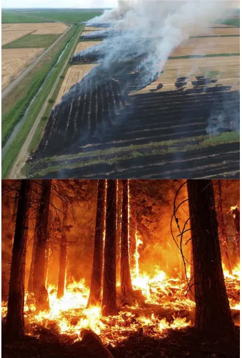
green-tip-limiting-outdoor-air-pollution/) ... 29 Figure 7 Flaming (bottom image) v. smoldering (top image) fire. Images obtained
from Google. ... 53 Figure 8 The yearly total number of fires, the yearly average fire radiative power
(and associated standard deviation), the yearly average brightness temperature (and associated standard deviation), the yearly burn area and the yearly ammonia emissions from fires plotted for 2005-2015. The associated trend line is displayed as a yellow-gold line. Error bars
represent the standard deviation.. ... 76 Figure 9 The monthly total number of fires, the monthly average fire radiative
power, the monthly burn area and the monthly NH3 emissions from
biomass burning for each year in the study.. ... 77 Figure 10 Comparing the predicted NH3 emissions with the calculated NH3
xi the one-to-one trendline where the calculated NH3 emissions =
the predicted SOM NH3 emissions. The gold line represents the
mean bias line and the purple line represents the median bias line... ... 80 Figure 11 Comparing the predicted NH3 emissions with the calculated NH3
emissions for 2014 on a log scale. The red line represents the one-to-one trendline where the calculated NH3 emissions = the predicted SOM NH3 emissions. The gold line represents the mean
bias line and the purple line represents the median bias line.... ... 82 Figure 12 Comparing the yearly total NH3 emissions (on a log scale) from
biomass burning calculated and predicted in this study with the NEI, the FINN and the GFED. Note that 2005 – 2009 and 2014 were not
included in the creation of the SOM... ... 83 Figure 13 Comparing the predicted NH3 emissions with the calculated NH3
emissions for 2010-2014 on a log scale. The red line represents the one-to-one trendline where the calculated NH3 emissions = the predicted SOM NH3 emissions. The gold line represents the
mean bias line and the purple line represents the median bias line... ... 100 Figure 14 The results from this work compared against other global biomass
burning emission inventories. It is important to note that the FINN
model does not quantify N2O emissions from biomass burning.... ... 102 Figure 15 Comparing ammonia emission inventories from biomass burning created
in this chapter (C3) and Chapter 2 (C2) with other major emission
inventories for the continental US. ... 106 Figure 16 Comparing NOx and N2O emission inventories from biomass burning
created in this chapter (C3) and Chapter 2 (C2) with other major emission
inventories for the continental US.. ... 107 Figure 17 Comparing burn areas obtained from the MODIS Collection
6 Burn Area product and the MODIS Collection 5.1 Burn Area
product for the CONUS.. ... 108
Figure 18 Comparing the yearly average calculated emissions of NH3, NOx and N2O (blue line) with the yearly average emissions predicted
xii Figure 19 Comparing current calculated average Nr emissions with projected
average Nr emissions based off two climate change scenarios: RCP 4.5. and RCP 8.5. The green diamonds represent the average emissions projected by the RCP 4.5 climate scenario, while the dashed green line represents the RCP 4.5 trendline based on current modeled average emissions. Similarly, the red diamonds represent future emissions projected by the RCP 8.5 climate scenario, with the dashed red line representing the trendline for RCP 8.5
projections based on the current average modeled emissions. The ‘Current’ time frame refers to the study period (2001 – 2015), ‘Mid-Century’ refers to 2050-2055 and ‘End of Century’ refers to
2090-2095... ... 118
Figure 20 Current global average temperature and precipitation and burn area compared with the global projected temperature, precipitation and burn area, respectively, for RCP 4.5 and RCP 8.5. The ‘Current’ time frame refers to the study period (2001 – 2015), ‘Mid-Century’
refers to 2050-2055 and ‘End of Century’ refers to 2090-2095... ... 121
Figure 21 Daily average concentrations of PM2.5 concentrations in New Delhi, India. The blue line represents the average daily concentrations of PM2.5 while the red line represents the Indian Ambient Air Quality
Standards for PM2.5. ... 131
Figure 22 Comparing Nr and OC emissions in the IGP (log scale) with average PM2.5
concentrations in New Delhi, India (linear scale)………...133
Figure 23 (a, top) NASA FIRMS active fire data (MODIS MCD14DL) plotted the 24-hour back trajectory (500m) for November 6, 2016, from the NOAA HYSPLIT model. The background image is a MODIS image from NASA’s Terra satellite for November 6, 2016, that shows smoke blanketing the region. (b, bottom) NASA FIRMS active fire data (MODIS MCD14DL) plotted the 24-hour back trajectory (500m) for May 29, 2016, from the NOAA HYSPLIT model. The background image is a MODIS
1 CHAPTER 1
Introduction
The biogeochemical cycling of nitrogen is extremely important due to the role nitrogen plays in both aquatic and terrestrial ecosystems. However, the increase in food and energy production is perturbing the global nitrogen cycle by increasing the availability of reactive nitrogen (Nr) species, where reactive nitrogen is defined as nitrogen that is biologically active, photo chemically reactive and/or radioactively active (e.g. ammonia (NH3), ammonium (NH4+), nitric oxide (NO), nitrogen dioxide (NO2), nitric acid (HNO3), nitrous oxide (N2O), nitrous acid (HONO), peroxyacetyl nitrate (PAN - CH3C(O)O2NO2), nitrate (NO3-), nitrite (NO2-),
hydroxylamine (NH2OH) and other organic N compounds) (Fowler et al., 2013). For this work, the focus is on emissions of ammonia (NH3), oxides of nitrogen (NOx; NOx = NO + NO2) and nitrous oxide (N2O). Increased emissions of reactive nitrogen in the atmosphere can negatively impact air quality, the environment and human health. For example, deposition of reactive nitrogen species can lead to a decrease in biological diversity, soil acidification and lake
eutrophication, eutrophication of coastal zones (Clark and Tilman, 2008; Galloway et al., 2004; Holtgrieve et al., 2011; Janssens et al., 2010; Phoenix et al., 2012; Erisman et al., 2013).
Atmospheric reactive nitrogen also has a negative impact on air quality. For example, NOx, a form of reactive nitrogen, can increase tropospheric ozone (O3) formation and NH3 can lead to the formation of fine particulate matter (PM2.5) (Baek and Aneja, 2004; Baek et al., 2004;
2 2009; Kwok et al., 2013; Crouse et al., 2015a; Crouse et al., 2015b; Lelieveld et al., 2015). PM2.5 is also associated with several environmental impacts, such as reducing visibility and changing the earth’s radiational balance (Fan et al., 2005; Behera and Sharma, 2010a; Behera and Sharma,
2010b, Heald et al., 2012; Wang et al., 2012). Increased emissions of reactive nitrogen can impact climate change as well as negatively impact human health and welfare (Davidson et al., 2012; Galloway et al., 2004; Gruber and Galloway, 2008).
Major sources of NH3 include nitrogen-based fertilizers, animal waste, and biomass burning (Langford et al., 1992; Schlesinger and Hartley, 1992; Bouwman et al., 1997; Delmas et al., 1997; Flechard and Fowler, 1998; Yu’e and Erda, 2000; Battye et al., 2003; Aneja et al., 2009; Syakila and Kroeze, 2011; Zbieranowski and Aherne, 2012). While agriculture accounts for approximately 82% of all ammonia emissions on a national level, fires account for a total of about 10% of all ammonia emissions nationwide, making it the second largest source of
ammonia into the atmosphere (2014 NEI). Biomass burning is an important source of ammonia emissions, but the strength of the source remains poorly quantified (Alves et al., 2011; Chen et al., 2014). Major sources of NOx include fossil fuel combustion (24%), mobile sources (57%) and industrial processes (10%) (EPA, 2016). Major sources of N2O include agriculture (80%) and combustion (10%) (EPA, 2016). While biomass burning only accounts for approximately 2% percent of all NOx and N2O emissions, it is still an important emission source of each species because it cannot be completely controlled.
The strength and frequency of fires are not only controlled by the properties of the fuel and the geography, but they are also influenced by weather and climate (Pyne et al., 1996; Liu et al., 2010). Therefore, changes in the earth’s climate will likely result in changes in fire activity
3 an increase in the number of observed wildfires across many regions of the US, such as the southeastern United States, the northern great plains, the Pacific coast, the southwestern US and the southern Rockies (Pinol et al., 1998; Gillet et al., 2004; Reinhard et al., 2005; Liu, 2006; Westerling et al., 2006; Alves et al., 2011; Litschert et al., 2012; Saylor et al., 2015; Skibba, 2015). However, due to changes in relative humidity and wind speeds, the future fire potential in the northern Rockies and the northwestern United States may likely be reduced (Liu et al., 2013). On a global scale, wildfire potential is projected to increase as the climate changes, specifically in locations that are already prone to the occurrence of wildfires (Liu et al., 2010). This increase in wildfire potential will then potentially lead to an increase in Nr emissions from biomass burning. These changes in the biogeochemical cycle of nitrogen will have great impacts on the environment. For example, gaseous ammonia may be deposited to the Earth’s surface, which leads to ammonification, eutrophication and a loss of biodiversity (Langford et al., 1992; Robarge et al., 2002; Galloway et al., 2004; Clark and Tilman, 2008; Janssens et al., 2010; Day et al., 2012; Holtgrieve et al., 2011; Phoenix et al., 2012; Erisman et al., 2013; Chen et al., 2014). Increased concentrations of ammonia can also lead to a decreased resistance to drought and frost damage (Robarge et al., 2002). In addition, nitrous oxide is a major greenhouse gas that
contributes to the warming climate (Bouwman, 1996).
The primary objective of this research is to quantify emissions of reactive nitrogen (NOx, NH3, N2O) from biomass burning (wildfires, agricultural burns and prescribed burns). The first analysis in this work focuses on quantifying NH3 emissions across the CONUS for 2005 – 2015 using a suite of satellite data (Chapter 2). This emission inventory was then compared against three major fire emission inventories: The Fire Inventory from the National Center for
4 Databases (GFED v4.1, with small fires; van der Werf et al., 2017), and the US Environmental Protection Agency (EPA) National Emissions Inventory (NEI) with fire inventory data.
Furthermore, a regression analysis, using forward stepwise regression, was completed in order to determine the best fit model of emissions for NH3 from biomass burning. The second analysis in this work (Chapter 3) is a global emissions inventory of three major reactive nitrogen species (NH3, NOx, and N2O) for 2001-2015. This inventory differs from the aforementioned CONUS inventory in the sense that it was created using an updated set of satellite data that are more representative of current conditions. This global inventory was then compared with both FINN (v1.4) and GFED(v4.1) on a year to year basis, while the yearly average was compared against the current literature. A regression analysis was also conducted for each species of reactive nitrogen and future emissions of each reactive nitrogen species were projected for 2050-2055 and 2090-2095 under two prominent climate change scenarios (RCP 4.5, RCP 8.5). Finally, a local scale analysis of Nr emissions from agricultural burning of wheat and rice paddy residue in the Indo-Gangetic Plains (IGP) in 2016 and 2017 was completed to determine the role of these emissions in ambient PM2.5 concentrations in New Delhi, India (Chapter 4). Using these data, statistical regression analyses were completed to predict ambient concentrations of PM2.5 in New Delhi based on both meteorological conditions and agricultural burning emissions of NH3 in the IGP.
1.1 - The Nitrogen Cycle
Nitrogen is an important and essential component of all life. However, most nitrogen in the atmosphere is molecular nitrogen (N2), which is an inert gas and therefore unused by
5 1995; Vitousek et al., 1997; Galloway, 1998; Seitzinger and Kroeze, 1998; Warneck, 1999; Galloway, 2000; Galloway and Cowling, 2002; Galloway et al., 2004; Galloway et al., 2008).
N2 gas in the atmosphere is very stable due to the nitrogen-nitrogen triple bond and takes an enormous amount of energy to break (940 kJ mol-1) (Gilchrist and Benjamin, 2017).
Therefore, the chemical conversion to biologically available forms (e.g. NO, NH3) is difficult. There are two types of natural processes for the fixation of N2 (Figure 1).
Figure 1. Major processes in the nitrogen cycle (Source: Warneck, 1999). One process is the conversion of N2 to NH3, NH4+ and organic nitrogen compounds via
microorganisms, while the other process is fixation of N2 (via lightning, cosmic rays) to produce NO in the atmosphere. Biological nitrogen fixation is done by prokaryotes, eubacteria and archea (diazotrophs) in anaerobic conditions due to the sensitivity of nitrogenase (the enzyme that is fixes N2) to oxygen. The importance of reactive nitrogen for agriculture was recognized and, therefore, the Haber-Bosch process began development in the early 1900s. The Haber-Bosch process, which is still used today, produces NH3 by reacting N2 and H2 at 300C and 300 atm
6 N2 + 3H2 → 2NH3 (R1).
Another contributor of fixed (reactive) biologically available nitrogen is the combustion of fossil fuels. Following the reduction of N2 to NH3 by diazotrophs, the NH3 is then assimilated as organic nitrogen via bacteria or the host plants (assimilation), which can then be consumed by animals (Jacob, 1999). These animals then excrete the consumed nitrogen or die and the resulting organic nitrogen is consumed by bacteria where it is then mineralized to NH4+, where it can be assimilated by other organisms. In addition to this, NH4+ can also be used by bacteria as an energy source by oxidizing it to nitrite (NO2-) or nitrate (NO3-) (nitrification) (Reactions 2-3; Gilchrist and Benjamin, 2017):
2NH4+ + 3O3 → 2NO2- + 4H+ + 2H2O + energy (R2), 2NO2- + O2 → 2NO3- + energy (R3).
As shown in the preceding reactions (Reactions 2 and 3), this process is aerobic (i.e. requires the presence of oxygen). Because nitrate is readily assimilated by plants and bacteria, it provides another route for the formation of organic nitrogen. Under anaerobic conditions (i.e. conditions lacking O2), bacteria use NO3- as an oxidant to convert NO3- to N2, which is then returned to the atmosphere in a complex, multi-step nitrogen reduction process:
7 It is important to note that emissions of NO and NO2 may also be released during this process (Gilchrist and Benjamin, 2017). While not shown in Figure 1, N2 may also be produced via anammox, which is an anaerobic ammonium oxidation pathway that was discovered in 1990 (Van de Graaf et al., 1990; Mulder et al., 1995; Jetten et al., 1998) due to high N2 generation at a waste water plant. The resulting studies showed that ammonium was able to be oxidized by certain bacteria using nitrite in anaerobic conditions (Reaction 4):
NH4+ + NO2- → N2 + 2H2O (R4).
Because this process converts biologically available nitrogen to N2, it can be considered as a form of denitrification. As aforementioned, N2 in the atmosphere can be fixed by high temperature oxidation to NO.
NO is formed in the atmosphere via processes either involving the oxidation of fuel nitrogen or by the oxidation of N2 at high temperatures. NO from combustion has several different formation mechanisms (Dean and Bozzelli, 2000; Erisman and Fowler, 2010): “Thermal NO” is formed under high flame temperatures (Zeldovich 1946), “Prompt NO” is
produced within fuel rich parts of flames (Fenimore, 1976), the “N2O mechanism” is important in high pressure flame (Wolfrum, 1972; Malte and Pratt, 1974), “Fuel nitrogen” NO is produced via the nitrogen containing species in the fuel (Fenimore, 1976), and the “NNH mechanism”
where NO is produced from high atom concentrations in flame fronts (Bozzelli and Dean, 1995). In the “Thermal NO” process, which is also called the Zeldovich mechanism, N2
8 O + N2 NO + N (R5)
N + O2 NO + O (R6)
N + OH NO + H (R7).
Due to the strong nitrogen-nitrogen triple bond, Reaction 5 requires a high activation energy (~320 kJ/mol) and is, therefore, extremely dependent on temperature.
The “Prompt NO” mechanism results in the rapid production of NO in a flame front,
where the concentration of hydrocarbon radicals is large. The hydrocarbon radicals react with N2 in a flame front to break the triple bond (Reaction 8):
CH + N2 HCN + N (R8),
allowing the free N atom to from the NO molecule from Reactions 5 and 6. Furthermore, HCN can lead to a second NO molecule.
The N2O pathway, which produces NO from N2O in the stratosphere, is as follows (Reactions 9-11):
O + N2 + M N2O + M (R9)
O + N2O 2NO (R10)
H + N2O NO + NH (R11),
where M is a “collision partner” that represents all the molecules present. Reaction 9 is more important at higher pressures.
9 N2 + H → NNH (R12)
O + NNH NO + NH (R13).
This production of NO is then followed by its oxidation to HNO3 (Reactions 14-17):
2NO + O2 2NO2 (R14)
3NO2 + H2O 2HNO3 + NO (R15)
2NO2 N2O4 (R16)
2NO2 + H2O HNO3 + HNO2 (R17),
which is then scavenged by rain. However, because industry is so prominent in some parts of the world, nitrogen fixation via combustion engines provides an increased amount of nitrogen to the biosphere that then leads to an additional fertilization effect. Nitrogen is transferred to the lithosphere via the burial of dead organisms at the bottom of the ocean that are incorporated into sedimentary rock (Jacob, 1999). The nitrogen in the sedimentary rock is released back into the atmosphere and thus closes the nitrogen cycle when it is brought back up to the surface of the continent and eroded (Jacob, 1999).
10 2004). Nitrogen fixation by anthropogenic activities contributed to a significant increase in reactive nitrogen emitted into the atmosphere, with energy production (e.g. fossil fuel
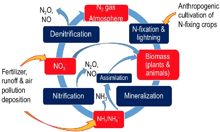
combustion, biofuel combustion, non-road transport), agriculture (e.g. fertilizer use, agricultural waste) and biomass burning contributing to the majority of Nr in the atmosphere. Battye et al. (2017) summarizes the anthropogenic perturbations to the natural nitrogen cycle with three general inputs: anthropogenic cultivation of nitrogen fixing crops, fertilizer run off and air pollution deposition (Figure 2, from Battye et al., 2017). Increases cultivation of nitrogen fixing crops (e.g. legumes) increased nitrogen fixation of atmospheric N2. In addition to this, the increased use of nitrogen fertilizer from the development of the Haber-Bosch process and the deposition of Nr species from fossil fuel combustion added to overall mass of biologically available nitrogen.
11 By the end of the 1900s, the anthropogenic contribution of reactive nitrogen exceeded the natural contribution of reactive nitrogen fixation in terrestrial ecosystems and current
anthropogenic inputs of reactive nitrogen may account for nearly half of the total reactive nitrogen flux on a global scale (Battye et al., 2017). This profound perturbation to the global nitrogen cycle is having a major impact on the environment, such as the emissions of precursor gases for PM2.5 and O3, impacts on species diversity, contamination of groundwater, and eutrophication.
1.2 - Reactive Nitrogen
As described above, reactive nitrogen is defined as species that are biologically active, photochemically reactive and/or radioactively active forms of nitrogen. The production of reactive nitrogen in the natural world occurs from the conversion of N2 to Nr, which requires a tremendous amount of energy due to the N2 triple bond. Therefore, terrestrial sources of reactive nitrogen include lightning and biological nitrogen fixation (BNF). Molecular oxygen and
nitrogen in the atmosphere produce NO when exposed to the high temperatures that occur during lightning strikes. This NO is then oxidized to NO2 and then HNO3 before being deposited back to earth via wet and dry deposition. Prior to the 20th century, anthropogenic reactive nitrogen was produced from fossil fuel, primarily coal, combustion and the cultivation of legumes. However, as the world’s population increased and the need for food and fiber increased, agricultural
12 were chosen due to their prominence (NH3 and NOx comprise half of the Nr emissions) and their impact on both human health and the environment.
1.2.1 - Ammonia (NH3)
Emissions
The exchange of NH3 between the biosphere and the atmosphere (the bi-directional flux) is dependent upon the concentrations of ammonia in the atmosphere and at the surface. As mentioned above, there are several sources of ammonia such as biomass burning, fossil fuel combustion, and human excreta (Aneja et al., 2012; Behera et al., 2013), however, agricultural sources of ammonia (e.g. volatilization of animal waste and synthetic fertilizers, losses from soil from agricultural crops) are dominant (Streets et al., 2003; Huang et al., 2012; Hauglustaine et al., 2014; US EPA, 2014; Riddick et al., 2016). Emissions from agriculture occur during animal housing, manure storage/spreading and when animals are grazing and are dependent upon the amino acid content of the animal food, the conversion efficiency of the N in the animal food (and thus the amount of N left in the manure), as well as the livestock age, weight and density. The emissions of NH3 from manure occur when the manure is exposed to air and the rate is
dependent upon the ambient concentration of NH3 above the manure. Ammonia emissions from animal livestock typically occurs from the decomposition of urea (mammals) or uric acid (birds) (Behera et al., 2013). NH3 emissions from animal livestock manure can be described using the following reactions (Reactions 18-23) (Behera et al., 2013):
13 NH4+ (aq, manure) NH3 (aq, manure) + H+ (R21)
NH3 (aq, manure) NH3 (g, manure) (R22)
NH3 (g, manure) NH3 (g, air). (R23)
In this process, Reaction 18 shows the aerobic decomposition of uric acid via microbial action (enzyme uricase) to produce CO2 and NH3, Reaction 19 shows urea hydrolysis and Reaction 20 shows the production of NH3 via the decomposition of undigested proteins by uricase and urease enzymes and bacterial metabolism (Behera et al., 2013). As mentioned above, the NH3 volatilization rate from livestock manure is dependent on both the ambient and surface concentrations of NH3, which is governed by Equation 1:
E = k(Cmanure – Cair) (1),
where, E is the volatilization rate (g m-2 s-1), k is the diffusion constant, Cmanure is the
concentration of ammonia at the surface (g m-2) and Cair is the ambient concentration of ammonia (g m-2), where the concentration of Cmanure is dependent upon the equilibrium between aqueous NH4+ (NH4+ (aq, manure)) and aqueous NH3 in the manure (NH3 (aq, manure)) (Reaction 21). The equilibrium between NH3 and NH4+ is dependent upon the ionic strength of the solution, which is determined via the dissociation constant (Ka) of Reaction 21, which is calculated using Equation 2:
𝐾𝑎 = [𝑁𝐻3][𝐻+]
[𝑁𝐻4+]
14 where the brackets, [ ], represent the molar concentrations. Temperature and pH both impact the equilibrium between [NH3] and [NH4+] (Behera et al., 2013). Finally, the formation of NH3 (g) in the atmosphere is dependent upon the equilibrium between NH3 (aq, manure) and NH3 (g,
manure) (Reaction 22) and the volatilization of NH3 from manure (NH3 (g, manure)) to the atmosphere (NH3 (g,air)) (Reaction 23). In addition to livestock, the use of synthetic fertilizers is another major source of ammonia emissions into the atmosphere. NH3 is transported into the atmosphere from the surface (either from within the soil surface or from plants) (Van der Molen et al. 1990; Sommer et al. 2004; Behera et al., 2013).
Following agriculture, biomass burning is the second largest emission source of NH3 in the CONUS (EPA, 2014). Because N is an essential ingredient in all proteins, it is present in all biomass in a reduced chemical state (e.g. amides (R– (C=O) – NH – R'), and amines (R–NH2) ) (Battye et al., 1994; Behera et al., 2013). N from biomass is primarily released as NH3 during biomass burning under poor mixing conditions. According to a study conducted by Yokelson et al. (1997), the majority of NH3 is emitted from visible glowing combustion, which is part of the smoldering stage of a fire. NH3 is also emitted naturally from soils from the decomposition of organic matter and from N compounds that hydrolyze to NH3 and NH4+. In addition to this under low concentrations of NH3, vegetation can act as a source. Conversely, under high concentrations of NH3, vegetation can act as a sink (Langford and Fehsenfeld, 1992). The primary driver of this exchange is the difference between the concentrations of NH3 in the atmosphere and the
15 NH3 emissions from vehicles come from two main sources: gasoline vehicles with three-way catalytic converters and diesel vehicles with the selective catalytic reduction system (Heeb et al. 2006; Pandolfi et al. 2012; Behera et al., 2013). Three-way catalytic converter vehicles emit NH3 as a result of NO reduction on the catalyst surface. In the selective catalytic reduction
system, urea is injected into the exhaust and then undergoes thermal decomposition and hydrolysis to form NH3 (Behera et al., 2013). Other minor sources of NH3 into the atmosphere include emissions from humans via sweat, breath, smoking and infant excretion (Healy et al., 1970; Lee and Dollard, 1994; Martin et al., 1997), emissions from wild animals, sea birds, horses and pets (Behera et al., 2013), and sewage emissions from anaerobic processes in the waste water treatment system and the spreading of treated sewage onto agricultural land (Harmel et al., 1997; Behera et al., 2013).
17 Table 1. Emission source categories identified by Van Damme et al. (2018) for regions shown in Figure 3.
REGION SOURCE TYPE
1 Eckley – Yuma (USA) Agriculture (cattle feedlot) 2 Bakersfield (USA) Agriculture (cattle feedlot) 3 Tulare (USA) Agriculture (cattle feedlot) 4 Torreon (Mexico) Agriculture (cattle feedlot) 5 Milford (USA) Agriculture (pig farms) 6 Alto Laran District (Peru) Agriculture (poultry housing) 7 Basmakci (Turkey) Agriculture (poultry housing) 8 Marvdasht (Iran) Industrial (fertilizer plant) 9 Pingsongxiang (China) Industrial (fertilizer plant) 10 Cherkasy (Ukraine) Industrial (fertilizer plant) 11 Sur Industrial Estate (Oman) Industrial (fertilizer plant) 12 Beech Island (USA) Industrial (fertilizer plant) 13 Ferghana (Uzbekistan) Industrial (fertilizer plant) 14 Talkha (Egypt) Industrial (fertilizer plant) 15 Abu Qir (Egypt) Industrial (fertilizer plant) 16 Secunda (South Africa) Industrial (fertilizer plant)
17 Shizuishan (China) Industrial (fertilizer and coal related industries) 18 Zezhou – Gaoping (China) Industrial (fertilizer and coal related industries) 19 Moa (Cuba) Industrial (Ni and Co mine/plant)
20 Nicaro (Cuba) Industrial (Ni and Co mine/plant) 21 Stuparei (Romania) Industrial (soda ash plant)
22 The Geysers (USA) Industrial (geothermal power plant) 23 Lake Natron (Tanzania) Natural (mud flats - algae decay) 24 Bacau (Romania) Industrial (fertilizer plant) 25 Chino (USA) Agricultural (cattle feedlots) 26 Wucaiwan (China) Industrial (fertilizer plant) 27 Anju (North Korea) Industrial (fertilizer plant) 28 Jharia (India) Industrial (burning coal mine)
Impacts
18 and hydrochloric acid to form ammonium sulfate/ammonium bisulfate, ammonium nitrate and ammonium chloride (Reactions 24-27, respectively):
2NH3 (g) + H2SO4 (g) ↔ (NH4)2SO4 (s) (R24) NH3(g) + H2SO4 ↔ NH4HSO4 (s) (R25) NH3 (g) + HNO3 (g) ↔ NH4NO3 (s) (R26) NH3 (g) + HCl (g) ↔ NH4Cl (s) (R27).
When compared with nitrate formation, the formation of sulfate is dominant during normal atmospheric conditions (Behera and Sharma, 2010a, b; Behera et al., 2013). The reaction rates are dependent upon the ambient temperature, humidity as well as the acid concentration and the NH4+ containing aerosols formed (Stelson et al., 1979; Huntzicker et al., 1980). It is also important to note that the formation of particulates can alter the earth’s radiational balance, by
scattering or absorbing solar radiation (Adams et al., 2001; Martin et al., 2004; Abbatt et al., 2006; Henze et al., 2012).
19 forest health in a number of ways, including soil acidification, nutrient imbalance, reductions in forest productivity and threats to forest biodiversity (Chiwa et al. 2004; Gaige et al. 2007; Sievering et al. 2007; Xiankai et al. 2008; Behera et al., 2013). Because NHx (NH3 + NH4+) are nutrients, deposition of NHx can also lead to eutrophication, which is an excessive richness of nutrients in bodies of water that cause a dense growth and plant life and thus the death of animal life from lack of oxygen (Aneja et al., 1986; Asman et al., 1998; Galloway et al., 2003; Erisman et al., 2005; Behera et al., 2013).
Trends
The increase in the world’s population will increase the use of fertilizer from the
agricultural industry, thus increasing ammonia emissions into the atmosphere (Aneja et al., 2006, 2008, 2009, 2012; Heald et. al., 2012). Butler et al. (2016) analyzed measurements from 18 long-term AMoN sites from 2008 to 2015 over large regions of the US at both a seasonal and an annual level of aggregation. The 18 sites used regions in the southeast, the northeast, the
20 observed. For all regions, the overall trend (i.e. the change in NH3 concentration over time) was found to be highly significant (p < 0.0001), with an overall +7% change in concentration at a 95% confidence interval. Similarly, Saylor et al. (2015) analyzed ammonia emissions from the Southeastern Aerosol Research and Characterization (SEARCH) network from 2004 to 2012. Starting in 2004, 24-hour integrated ammonia measurements were taken at eight sites using a citric acid-impregnated 242-mm annular denuder on a 1 in 3-day sampling schedule (Saylor et al., 2015). In addition to this, integrated 24-hour PM2.5 measurements were also taken using a multichannel particle composition monitor (PCM). These measurements were analyzed for mass, major inorganic ions, trace elements, organic carbon and light-absorbing carbon (Saylor et al. 2015). The results of this study showed an overall decrease (1-4% per year) in the total ammonia concentrations (i.e. gas phase ammonia + particulate ammonium). However, an increase in gas phase ammonia mixing ratios was observed throughout the region, thus the gas phase fraction of total ammonia has increased during the period. Saylor et al. (2015) attributes this to the decline of sulfur dioxide and nitrogen oxide emissions (Xing et al., 2013), which is reducing the partitioning of to the fine particle phase. In addition to this, Saylor et al. (2015) attributes the unusually high ammonia concentrations observed in 2007 to emissions from wildfires. Butler et al. (2016) also evaluated particulate ammonium concentrations from the NADP National Trends Network (NTN) and the NADP Atmospheric Integrated Research Monitoring Network
21 The use of satellite IR sounders has greatly improved the capability to quantify
atmospheric NH3 from space. For example, Warner et al. (2017) used the Atmospheric Infrared Sounder (AIRS) to observe changes in the global ambient concentration of NH3 over agricultural regions from 2002 to 2016 and found increases concentrations over the midwestern part of the US (~2. 61% yr−1), the European Union (~1.83% yr−1) and in China (~2. 27% yr−1) that are statistically significant at the 95% confidence level with p-values of 0.0003, 0.0028 and 0.026, respectively. In addition, a slight increase in emissions was also observed over South Asia, however, the increase was not statistically significant (p-value = 0.61). Clarisse et al. (2009), used the Infrared Atmospheric Sounding Interferometer (IASI) to retrieve atmospheric ammonia at a global scale for 2008 and concluded that global emissions have more than doubled since industrial times.
There is also a seasonal trend in ammonia emissions and ambient concentrations. Seasonal changes in ammonia emissions are primarily due to changes in both agricultural and burning practices as well as changes in the meteorology. While seasonal changes in
22 concentrations of nitrate tended to be higher in the winter than in the summer time (Aneja et. al., 2006; Behera and Sharma, 2010a, b; Lonati et. al., 2004; Huang et. al., 2009). There are several factors that are likely contributors to this finding. A major factor is due to the meteorology of the wintertime. Temperatures are colder and the boundary layer is lower. Because Reaction 9 is temperature dependent, it is more prominent in the winter time because the lower temperatures favor the shift from the gas phase of HNO3 to the particle phase of NH4NO3, which could lead to higher concentrations of NO3- in the winter (Behera and Sharma, 2010a, b). In addition to this, increased coal and fossil fuel combustion for heating during the winter months contribute to additional NOx emissions in the atmosphere, which are necessary for the formation of NO3-. Modeling
Despite the importance of atmospheric ammonia, emissions are poorly quantified. Due to uncertainties in ammonia emissions sources and the relatively short lifetime of gaseous ammonia in the atmosphere, modeling concentrations of atmospheric ammonia is a challenging endeavor. A study was conducted by Bray et al. (2017) (Appendix A) to evaluate how well the U.S.
23 Kelly et al., 2014; Butler et al., 2015; Schiferl et al., 2016; Battye et al., 2016). Gilliland et al. (2006) used an inverse modeling technique with CMAQ v4.4 to predict NH3 emissions for the continental United States (CONUS). The results of Bray et al. (2017) indicated that the emissions inventory is too high for the winter months and too low for the summer months. Similar results were found by Butler et al. (2015), who used CMAQ v4.7.1 to predict NH3 concentrations in Susquehanna River Watershed of New York and Pennsylvania. When comparing ambient concentration measurements of NH3 with the model predictions, it was found that the model under estimated concentration by 8-60%. In addition to this, it was also found that the NH3 under estimations were particularly high over the agricultural regions. Kelly et al. (2014) found similar results when comparing NH3 measurements obtained from the California Research at the Nexus of Air Quality and Climate Change (CalNex) field campaign that occurred May-June, 2010, with model predictions from CMAQ v5.0.2. In addition to this, it was also found that the CMAQ model also predicted lower concentrations of NH3 in some urban regions as well. Battye et al. (2016) found comparable results to Kelly et al. (2014) when comparing NH3 measurements from the Deriving Information on Surface conditions from Column and Vertically Resolved
Observations Relevant to Air Quality (DISCOVER AQ) field campaign (July-August, 2014) with NOAA’s NAQFC CMAQ model (v5.0.2) over the agricultural regions of northeastern
24 estimates NH3 concentration, with the results being most comparable to Kelly et al. (2014) and Battye et al. (2016).
Figure 4. Aircraft in-situ measurements of NH3 (blue dots) plotted against model predictions on a log-log scale plot. The red line shows where the measured points should have fallen if the model predictions were exactly correct and the gold line shows the actual measured trend line. The actual trend line (gold line) is plotted above the one-to-one line (red line), while the bias line given by the median ratio is given by the cyan-green line. Figure obtained from Bray et al. (2017).
1.2.2 - Oxides of Nitrogen (NOx) Emissions
NOx is produced from the reaction of nitrogen and oxygen in the atmosphere during combustion. There are several sources of NOx (NO + NO2) at the surface, such as mobile
25 fuel combustion, biomass burning and biogenic emissions from the soil are the three primary sources of NOx. The primary emission of NOx in the atmosphere is in the form of NO. As discussed above, there are two nitrogen sources that contribute to the formation of NO (i.e. the primary N product of fossil fuel combustion): atmospheric N2 and organic nitrogen in the fuel. The Zeldovich mechanism explains the formation of NO via atmospheric N2 (Zeldovich, 1947; Delmas et al., 1997):
N2 + O → N + NO (R28) N + O2 → NO + O (R29),
where, Reaction 28 requires a high activation energy. The formation of NO from organic
nitrogen is more complicated. Organic compounds are released during combustion as animes and cyanides which are then oxidized into NO by free radicals (e.g. OH, O) or reduced to N2 by a nitrogenous co-reagent (e.g. NO). Because the triple bond of molecular nitrogen is so strong, the NO formation velocity is much higher from organic nitrogen (Delmas et al., 1997). The other surface NOx source is biomass burning. NOx is emitted in the form of NO during the flaming phase of combustion. The amount of NOx emitted is not only directly related to the fire
properties, but the fuel properties (e.g. biomass loading, fuel type, moisture content) as well. As with NH3, the organic nitrogen in the fuel provides the source of nitrogen compounds emitted into the atmosphere during combustion.
26 rates of nitrification and denitrification, which is determined by the physical and chemical
conditions of the soil (e.g. texture, temperature, moisture content, oxygen content, pH). For example, NO can be produced adiabatically from the chemical decomposition of nitrites under low pH and high organic matter conditions (Delmas et al., 1997). In addition to this, the application of nitrogen fertilizer is usually associated with NO emissions, with the intensity of emissions varying based on the response of the system (Delmas et al., 1997). The NO emitted into the atmosphere can then be oxidized to form atmospheric NO2 via Reaction 30:
2NO + O2 → 2NO2 (R30).
Other industrial processes that emit NOx into the atmosphere include paving roads with asphalt and the manufacturing of adipic acid, nitric acid, iron and steel, aluminum and pulp and paper board products (Yu’e and Erda, 2000).
Tropospheric sources of NOx include lightning, stratospheric injection, ammonia
oxidation and aircrafts (Delmas et al., 1997). Each bolt of lightning produces NO gas, which can then react with molecular oxygen to form NO2. In addition to this, NOx produced in the
stratosphere can be injected into the troposphere. NO is produced in the stratosphere from the oxidation of N2O (Delmas et al., 1997; Warneck, 1999):
27 Furthermore, aircrafts also inject NOx, along with other pollutants, into the troposphere (Gauss et al., 2006). Finally, the oxidation of ammonia, which is initiated via Reaction 34:
OH + NH3 → NH2 + H2O (R34),
can be a potential sink or source for NOx because the NH2 radical can react with O3 to form NO or it can react with NO and NO2 to form other products (Delmas et al., 1997; Seinfeld and Pandis, 2006).
van der A et al. (2008) used the GOME(Global Ozone Monitoring Experiment) and SCIAMACHY (SCanning ImagingAbsorption spectroMeter for Atmospheric CartograpHY) satellite instruments to determine the global distribution of NO2 in the troposphere (Figure 5, from van der A et al., 2008) as well as emission sources at the global scale. The results of this study identified three categories of emission sources: anthropogenic, biomass burning and soil. Anthropogenic emissions of NOx occur in industrial regions, such as the US, eastern China, Japan and South Africa. Biomass burning emission of NOx are prominent in the African savannas, while emissions from soil occur in regions consisting of grassland and sparsely
28 Figure 5. Mean tropospheric NO2 column for 2004 derived from SCIAMACHY observations (source: van der A et al., 2008)
Impacts
There are several health and environmental impacts associated with NOx in the atmosphere. Exposure to elevated NOx concentrations can impact the respiratory system by causing inflammation, decreasing lung function as well as cause emphysema like lesions (Chauhan et al., 1998; Kampa and Castanas, 2008).
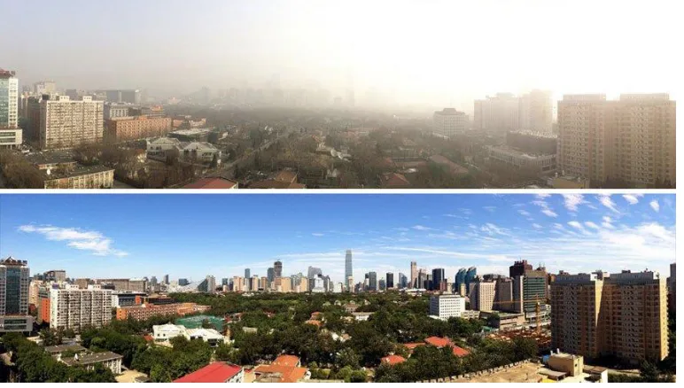
29 Figure 6. Example of photochemical smog (top) in California compared with a clear
day(bottom). (Source: http://www.topsmkt.com/going-green/tops-june-green-tip-limiting-outdoor-air-pollution/)
The general, simplified smog formation chemistry is as follows (Reactions 35-41): NO + O2 → NO2 + O (R35)
NO2 + h → NO + O (λ < 397 nm) (R36) O + O2 → O3 (R37) O3 + NO → O2 + NO2 (R38) RC + O → RCO (R39)
RCO + O2 → RCO3 (R40) NO + RCO3 → NO2 + RCO2 (R41).
30 it is important to note that a variety of other molecules can also act as a catalyst for this reaction. Tropospheric ozone can react with NO to produce O2 and NO2 (scavenging reaction) (Reaction 38). This reaction typically occurs in the evening hours and, due to lack of sunlight, leads to a reduction in ambient ozone concentration. In addition to NOx, hydrocarbons (RC) are also important. RC combined with O forms RCO (Reaction 39), which represents a number of different aldehydes and ketones. Some of which can react with O2 to form peroxide radicals (RCO3) (Reaction 40). RCO3 reacts with molecular oxygen to form O3 and RCO2 or they can react with NO to form NO2 and RCO2 (Reaction 41).
As observed in Reactions 34-37, NOx also contributes to the formation of tropospheric ozone, which is associated with a wide array of health and environmental impacts. Exposure to elevated concentrations of ozone is known to lead to several cardiovascular and respiratory issues, such as pneumonia, pulmonary disease and asthma (Gryparis et al. 2004; Mudway and Kelly, 2000). In addition to this, exposure to elevated concentrations of ozone can also
negatively impact vegetation by reducing agricultural and forest yields, reducing growth and increasing the susceptibility of the vegetation to diseases. Furthermore, exposure to ozone can also deteriorate rubber and damage buildings (Mauzerall and Wang, 2001).
NOx is also a precursor gas for secondary particulate matter. NO2 contributes to the formation of ammonium nitrate, which is a major inorganic constituent of PM2.5, via Reactions 42-43:
31 As discussed above, particulate matter is also associated with a number of health and environmental impacts. Exposure to high concentrations of particulate matter can also lead to cardiovascular and respiratory issues (Dominici et al. 2006; Ibald-Mulli et al. 2002; Pope et al. 2002; Pope and Dockery, 2006; Pope et al., 2009). Particulate matter also can reduce visibility, damage and/or stain material and, depending on the composition of the PM, can even contribute to acid rain, change the nutrient balance of aquatic ecosystems, damage crops and forests and contribute to acidification of both soil and water.
Not only is NOx important in daytime atmospheric chemistry, but both NO and NO2 play an important role in night time atmospheric chemistry as well through the formation of the nitrate radical (NO3) and dinitrogen pentoxide (N2O5) (Reactions 44-46; Jacobson, 2012).
N2 + O3 → NO3 + O2 (R44)
NO2 + NO3 N2O5 (R45) N2O5 + H2O → 2HNO3 (R46).
The night time chemistry of NO3 and N2O5 is extremely important for both the atmospheric ozone and reactive nitrogen budgets, the oxidation of biogenic volatile organic compounds and in the formation of atmospheric aerosols (Brown and Stutz, 2012).
Trends
32 emissions in recent years. For example, measurements from continuous emission monitoring systems (CEMS) from 1997 to 2013 suggest a 40% reduction in NOx emissions (de Gouw et al., 2014). Similar results were found by Lu et al. (2015), who determined trends in NOx emissions from 2005 to 2014 using retrievals from the Ozone Monitoring Instrument (OMI) and found that emissions of NOx in urban areas have decreased by nearly 50%, which is consistent with bottom up emission estimates and averaged NO2 concentrations from monitor data over the period. Reis et al. (2009) also observed a decrease in NOx emissions from 1990 to 2005 based on emission data from EDGAR and the US EPA NEI. Observational data from the AQS for 1990 to 2010 show an average annual decrease of 2.3% for NO2 for the US (Xing et al., 2015). Tong et al. (2015) used OMI NO2 retrieval data and EPA Air Quality System (AQS) ground data to
33 trends. A significant reduction in NO2 was observed in Europe and the eastern US while a
significant increase was observed for much of Asia. Modeling
Accurate quantification of NOx emissions is crucial in emission modeling of NOx. However, getting an accurate quantification of emissions on a national scale is challenging. For example, Houyoux et al. (2000) found a poor correlation when comparing average non-methane organic gases to NOx ratios from emission inventory derived from the 1990 and 1995 Ozone Transport Assessment Group (OTAG) with observed data from the Photochemical Assessment Monitoring Stations (PAMS). In another study, Boersma et al. (2008) estimated NOx emissions over the US using NOx retrievals from the Ozone Monitoring Instrument (OMI) with GEOS-Chem and compared their results with the 1999 US EPA NEI and found that the NEI
34 observations, but the Houston plumes were overestimated by about 60%. These results coincide with Rivera et al. (2010), who quantified NOx emissions in the Houston Ship Channel and found emissions to be approximately 70% higher than the emissions quantified in the Texas
Commission on Environmental Quality 2006 emission inventory.
35 very different top down emission inventories (Kemball-Cook et al., 2015). This is an important finding because satellite retrieval data is becoming increasingly more popular.
Because NOx plays such a crucial role in the formation of tropospheric ozone, which is one of the US EPA’s criteria pollutants, a number of studies have been conducted in order to see
36 1.2.3 - Nitrous Oxide (N2O)
Emissions
N2O is a colorless gas that is primarily emitted into the atmosphere via biological sources in the soil and water. Agricultural sources (80%), fossil fuel combustion (10%) and industrial activities (8%) are the most prominent emission sources of N2O. The emissions from the soil primarily occur from microbially driven nitrification (nitrate to nitrite) and denitrification (oxidation of ammonia), coupled with non-biological chemodenitrification (the chemical
37 In addition to this, industrial processes, combustion and municipal waste can also emit N2O into the atmosphere. For example, according to Yu’e and Erda (2000), the primary industrial sources of N2O into the atmosphere are adipic acid and nitric acid manufacturing. In addition to this, Strokal and Kroeze (2014) suggest that increasing urbanization may lead an increase in N2O emissions from human waste. Biomass burning is another important source of N2O into the atmosphere. Similar to the emission of NOx via biomass burning, N2O also tends to be emitted during the flaming phase of combustion and the amount emitted is highly dependent upon the characteristics of the fuel (e.g. moisture content, fuel type, fuel arrangement) (Lobert, 1991; Yokelson et al., 1997; Chen et al., 2007; McMeeking et al., 2009; Burling et al., 2010; Urbanski, 2014).
Impacts
While inert in the troposphere, atmospheric N2O plays a significant role in stratospheric chemistry, the radiational balance of the earth as well as in the global nitrogen cycle (Badr and Probert, 1993). A major impact associated with N2O is its warming potential. Per molecule, N2O has a warming potential of 200-300 times that of CO2 (Mosier et al., 1998; Forster et al., 2007). Greenhouse gases warm the atmosphere by absorbing the earth’s radiational energy, as oppose to
letting it escape back to space. Therefore, increased concentrations of N2O contribute to an increase in the warming of the earth’s atmosphere, which can in turn negatively impact the
environment. For example, rising temperatures can result in a longer growing season which will then lead to changes in agricultural activity as well as changes to delicate ecosystems.
Precipitation patterns are expected to change. For example, the northern US will likely observe more precipitation in the winter and spring, while droughts are expected to increase in the
38 will lead to drier soil and thus impact agriculture. Both heat waves and droughts contribute to favorable conditions for wildfire activity. Other potential impacts of the warmer climate include an increase in the frequency and intensity of hurricane activity in the Atlantic Ocean, however, this contribute of human activity to the recent changes in hurricane activity is fairly uncertain, and an increase in sea level which is a result of melting land ice as well as the expansion of sea water. There will be regional differences in the changing climate across the US. The northeastern US will likely see an increase in heat waves and heavy rains and the rising sea level will also likely pose a threat. This will lead to problems with agriculture, infrastructure, fisheries as well as ecosystems. In the northwest, shorter frost seasons will lead to changes in streamflow and a reduction in the water supply. In addition to this, the rising sea level and increased ocean acidity will impact fishing, lead to erosion as well as damage coastal infrastructure. Furthermore, warmer and drier conditions will increase the risk of wildfire, lead to insect outbreaks as well as an increase in tree disease. Sea level rise also poses a threat to the southeastern US. In addition to this, extreme heat and decreased water availability will impact human health as well as
agriculture, among other things. The Midwest is also expected to see extreme heat, in addition to heavy rains and flooding. This will cause major problems with infrastructure, health, agriculture and forestry, as well as reducing both air and water quality. In contrast to this, the southwest is expected to observe warmer and drier conditions that will increase wildfire activity, reduce water supplies and agricultural yields.
39 regulations of N2O emission sources. In the stratosphere, the Chapman cycle is the dominant source of ozone, and thus of the ozone layer (Reactions 43-45, Warneck, 1999):
O2 + h → 2O (180 nm < λ < 240 nm) (R43)
O2 + O → O (R44)
O3 + h → O2 + O (200 nm < λ < 300 nm) (R45).
However, N2O contributes to NO in the stratosphere (Reactions 46-48):
N2O + h → N2 + O (λ < 220 nm) (R46)
N2O + O → N2 + O2 (R47) N2O + O → 2NO (R48),
which then contributes to the destruction of the ozone layer via Reactions 49-50:
NO + O3 → NO2 + O2 (R49) NO2 + O3 → NO + 2O2. (R50).
The destruction of the stratospheric ozone layer increases the ultraviolet (UV) radiation that reaches the earth’s surface. This results in an increase in skin cancer, damage to the human
40 cycling of different elements (e.g. N, C). Furthermore, UV radiation also can alter certain
materials, such as synthetic polymers. Trends
41 explained by the emission inventories based on IPCC guidelines because the global estimated emissions are too low to explain current trends (Syakila and Kroeze,2011).
Olivier et al. (2005) used the Emission Database for Global Atmospheric Research (EDGAR) to determine trends in greenhouse gas emissions. According to Olivier et al. (2005), while global N2O emissions are increasing from agricultural sources and biomass burning (slight increase), they are decreasing from nitric and apidic acid manufacturing. However, on average, emissions of N2O have increased 3% from 1995 to 2002 and 4% from 2000 to 2003. Reis et al. (2009) observed a reduction in N2O emissions based on data from EDGAR and the US EPA NEI for 1990 to 2005. However, despite improvements in the efficiency of nitrogen fertilizer used in agriculture, agricultural emissions of N2O increased from 2002 to 2009 in the US (Cavigelli et al., 2012).
Modeling
N2O is an extremely important greenhouse gas with a large energy absorption capacity per molecule and a warming power that is 300 times the warming power of CO2 (Seinfeld and Pandis, 2006) and the changing climate has contributed to major changes in the global
42 from 2000-2010 using the Dynamic Land Ecosystem Model under six climate scenarios. Abalos et al. (2016) used a process-based model to determine the impact high and medium IPCC climate change scenarios would have on grasslands in South West England and found emissions would increase up to 94% of the baseline with the changing climate.
Agricultural sources are currently the largest source of N2O emissions and therefore the greatest contributor to N2O concentrations in the atmosphere. Therefore, changes to agricultural practices would lead to a reduction in emissions. While the climate projections simulated by Abalos et al. (2016) showed an increase in N2O emissions (up to 94% higher than baseline), they also found that replacing ammonium-nitrate fertilizers with urea or slurry resulted in a ~30% reduction in emissions. He et al. (2018) used the DNDC model to see how N2O emissions from crop fields would change in Ontario, Canada. They found emissions of N2O from winter wheat increased 17-38% with general practices. However, using higher crop heat units (note: crop heat units is a system that assists farmers in choosing suitable hybrids and varieties for their area) cultivars during the longer growing season resulted in a reduction in N2O emissions and an increase in wheat crop yields.
1.3 - Biomass Burning as a Source for Reactive Nitrogen
Biomass burning, which for this work includes wildfires, prescribed burns and
43 other pollutants including greenhouse gases (e.g. N2O), photochemically active compounds (e.g. non-methane volatile organic compound (NMVOC), NOx), NH3 and particulate matter (PM) (Hegg et al., 1988; Bouwman et al., 1997; Bouwman et al., 2002; US EPA, 2014; Whitburn et al., 2015).
Emissions from biomass burning and thus the impact fires have on air quality are
dependent on several different factors, including the combustion process. Ignition of combustion, which is essentially a rapid reaction of oxygen with a burnable substance that produces heat and light, requires the presence of three things: heat, oxygen and fuel (the fire triangle). Fires are directly related to the three elements in the fire triangle. For example, the removal of one element will extinguish the fire, while the weakening of one element will weaken the fire.
There are several phases of combustion, with the four most important being pre-ignition, flaming, smoldering and glowing. During pre-ignition, volatile materials in the fuel are
44 first mechanism is the fuel NOx mechanism, where fuel bound nitrogen produce nitrogen
generates gas-phase intermediate species (e.g. HCN) that is then oxidized to form NO or reduced to form N2, however, the details of the kinetics are not well understood (Baxter et al., 1995). Both the thermal NO mechanism and the prompt NO mechanism are discussed in Section 1.1 and are represented by R5-R8. In addition to this, NO2 can also be formed in flames via:
NO + HO2 → NO2 + OH (R51) NO + RO2 → NO2 + RO (R52),
where RO2 represents hydrocarbon peroxides. These reactions can subsequently lead to NO formation via:
NO2 + CN → NCO + NO (R53) NO2 + OH → HO2 + NO (R54)
NO2 + H → NH + NO (R55)
NO2 + O → O2 + NO (R56)
NO2+M →O + NO + M (R57).
The major pathways to produce N2O from biomass burning include:
NH + NO → N2O + H (R58)
O + N2 + M → N2O + M (R59),
45 NH3, methanol, formic acid, acetic acids and formaldehyde (Bertschi et al., 2003; Yokelson et al., 1996; Yokelson et al., 1997). NH3 from biomass burning results from the pyrolysis of amides (R– (C=O) – NH – R') and amines (R–NH2) ) (Battye et al., 1994; Behera et al., 2013). NH3 can also be formed in the atmosphere from the reaction of isocyanic acid (HNCO), another
byproduct of combustion, and water (H2O) (Haidar et al., 1981; Tsang, 1992): HNCO + H2O → NH3 + CO2 (R60)
The final phase is glowing combustion, which is when only the embers are visible and occurs at the end of the smoldering phase. This process primarily emits CO and CO2 and ends when pyrolysis can no longer occur (Simmons, 1995)
The quantity and composition of emissions emitted during each combustion process are dependent upon several factors, such as the fuel characteristics (e.g. the type of fuel, the fuel moisture, the fuel arrangement) as well as the fire behavior, which is a function of the meteorological conditions and topography (Albini, 1976; Anderson, 1983; Rothermel, 1972; Christian et al., 2003). In general, biomass material burned is composed of approximately 40% carbon, 6.7% hydrogen and 53.5% oxygen, with nitrogen accounting for 0.3-3.8% and sulfur accounting for 0.1-0.9%, depending on the type of biomass (Levine, 1994). Different fuel
arrangements, conditions and types tend to favor certain combustion processes (Urbanski, 2014). For example, large woody fuels (e.g. logs, stumps) and ground fuels (e.g. peat, organic soil) tend to favor smoldering conditions, while fine woody fuels, grass and foliage favor flaming
46 while smoldering combustion produces CO, CH4, NH3, NMOC and organic aerosols (OA)
(McMeeking et al., 2009; Burling et al., 2010; Urbanski, 2014). However, some NMOC species have been linked to both smoldering and flaming combustion processes. It is also important to note that the composition of the fuel (i.e. the nitrogen (N), sulfur (S) and chlorine (Cl) content) is also important in constituents emitted (Burling et al., 2010; Urbanski, 2014).