Article
1
Heat Pump Dryer Design Optimization Algorithm
2
Bernardo Andrade 1,3, Ighor Amorim 2,3, Michel Silva 2,3,6, Larysa Savosh 4, Luís Frölén Ribeiro 3,5,*
3
1 CEFET-MG – Brazil
4
2 UTFPR – Ponta Grossa - Brazil
5
3 Mechanical Technology Department - Polytechnic Institute of Bragança – Portugal
6
4 Lutsk National Technical University – Ukraine
7
5 Centre for Renewable Energy Research - INEGI – Portugal
8
6 Team4cooling – Portugal
9
10
* Correspondence: [email protected]; Tel.: +351-273303148 (L.F.R.)
11
12
Abstract: Drying food involves complex physical atmospheric mechanisms with non-linear
13
relations from the air-food interactions and those relations are strongly dependent on the
14
moisture contents and the type of food. Such dependence makes it complex to design suitable
15
dryers dedicated to a single drying process. To streamline the design of a novel compact
food-16
drying machine, a heat pump dryer component design optimization algorithm was developed
17
as a subprogram of a Computer Aided Engineering tool. The algorithm requires inputting food
18
and air properties, the volume of the drying container and the technical specifications of the
19
heat-pump off-the shelf components. The heat required to dehumidify the food supplied by the
20
heat exchange process from condenser to evaporator, and the compressor’s requirements
21
(refrigerant mass flow rate and operating pressures) are then calculated. Compressors can then
22
be selected based in the volume and type of food to be dried. The algorithm is shown via a flow
23
chart to guide the user through 3 different stages: Changes in drying air properties, Heat flow
24
within dryer and Product moisture content. Example results of how different compressors are
25
selected for different type of produces and quantities (Agaricus Blazei mushroom with 3 different
26
moisture contents or fish from Thunnini tribe) conclude this article.
27
Keywords: Algorithm; Heat-Pump; Drying; Food; Design; Optimization
28
29
1. Introduction
30
Food drying is one of the strategies for food preservation, and one of several strategies is the
31
thermal based mechanism, which is complex and involves the removal of a solid product`s moisture
32
by the employment of heat. The drying occurs through heat and mass transfers while the properties
33
of the food change throughout the process. There are many different machines that can make this
34
process, one of these is heat-pump based [1].
35
This machine extracts energy via a gas compressor from a cold-source and delivers it to a
hot-36
source. It does so by providing work to the refrigerant fluid. The heat-pump provides heat, making
37
it directly useful for heating ventilation and air conditioning (HVAC), but also for drying applications.
38
The machine energy input is the energy received from the compressor and adds it to the amount of
39
energy removed from the cold-source, yielding a higher energy output. As an example, for a
40
compressor yielding 100 W to remove 400 W from a cold-source, the total amount of energy provided
41
to the hot-source will be 500 W. This is a 5-time higher value than the one extracted by the compressor,
42
meaning a 500 W heating service from a 100 W electrical input. This highlights the energy saving
43
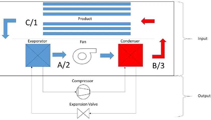
feature of this technology. A scheme of the whole machine and its components is shown in Fig 1:
44
compressor, expansion valve and heat exchangers (condenser and evaporator).
45
46
The work cycle starts with the air being heated at the condenser after being blown towards the
47
product (A to B in Fig.1). When the warm air passes by the food, it removes moisture from the
48
material. Downstream, the air captured the moisture from the food (B to C in Fig.1) and proceeds to
49
the evaporator, to partially condense some of its water. This (C to A in Fig.1) is achieved by promoting
50
the heat transfer of the air with the surfaces of the evaporator colder than the dew-point of the air.
51
For a real machine a percentage of outside air replaces part of the circulating air at each pass to allow
52
the cooling elements to condense more moisture from the air and to avoid the increase in temperature
53
of the circulating air.
54
55
56
Figure 1. Scheme of a specific prototype of a heat pump food dryer tested for this algorithm
57
where the thin line represents the refrigerant circuit while the thick arrows represent the air-flow
58
circuit.
59
60
The design of this machine for different purposes, or types of food, can be improved by the
61
application of resources such as the numerical optimization. Improving equipment design takes time
62
and laboratorial costs which are not directly translated towards the manufacturing process, for the
63
material acquired is usually spent on tests. Mathematical and computational mechanics models are
64
effective alternatives to many practical experiments since they provide a prediction of what may
65
happen and what can be expected. This approach allows for greater comprehension of the transport
66
phenomena involved in the drying of food, sharpens testing and production leading to a better and
67
quicker design process [2].
68
A simulation can also have an edge on normal experiments for it can predict, with virtual sensors,
69
the humidity, air velocity and temperature on points that are normally inaccessible since the presence
70
of the sensors would impact the air circulation inside the drying container. Also, there is no limitation
71
of testing different working conditions, there is no space restriction nor need for trained operators.
72
However, simulations require reliable data and proper modelling, otherwise the quality of results
73
may be questionable. This is true for the case of drying food especially describing the
74
physical/chemical properties and transport phenomena.
75
To achieve better results in energy efficiency and product quality, studies have been performed
76
in this area and new, more efficient models of heat-pump dryers have been created [2,4]. And so, the
77
use of algorithms comes into play as the driving force of better product design, enabling the creation
78
An algorithm is proposed in this article to aid the selection of heat-pump components. It is
80
presented through a flow chart that helps the designer visualize and comprehend the specified
81
numerical solution`s steps. A code was created to test the algorithm and how its results help the
82
development of different size drying machines. Examples from 2 different produces and how they
83
determine compressor selection (outputs) are later discussed.
84
2. Materials and Methods
85
The design algorithm is a logic map of efficient design of food-drying heat-pump air-based
86
machines. The algorithm inputs are the type of food, the air properties and the dimensions of the
87
food container, as well as the dryer component properties. To guarantee the temperature control
88
throughout the drying process, the working temperature of the air to which the food is being exposed
89
to is used as input. Therefore, it is possible to ascertain the final product quality, since over-heating
90
could cause damage to the product. Meanwhile, the algorithm outputs the mass flow of refrigerant
91
fluid from which the compressor and expansion valve can be selected. The difference of the algorithm
92
inputs and outputs, and their relation to the machine design are depicted in Fig.1. In this figure within
93
the circulating air volume there are 2 different nomenclatures aiming the description of different
94
things: A, B and C are related only to the air properties; 1, 2 and 3 represent the 3 stages of the
95
algorithm, with different transport and energy equations.
96
1. Changes in drying air properties;
97
2. Heat flow within dryer;
98
3. Product moisture content.
99
2.1. Stage 1 of the algorithm
100
The first stage of the algorithm determines the psychrometric and dynamic states of the air. The
101
literature recommends temperatures for drying each food, and by using them in the following
102
psychrometric and transport equations, one obtains every property necessary to the characterization of
103
the process and posterior steps [5–7].
104
The calculus of the air properties are given by Eq. (1) to (17). The specific psychometry Eq. (1-8) are
105
recommended by [6]. The psychrometric equations utilized at this stage describe the humid air based
106
on its temperature, amount of water as vapor and the air`s occupied volume [8–10].
107
To provide the readers less clutter information on the variables of the equations, a list of variables
108
and units is shown in the end of the article.
109
At first it is necessary to obtain the vapor saturation pressure 𝑃𝑣𝑠 and the absolute humidity 𝑤.
110
The air humidity after the contact with the food in the first iteration and after the air leaves the
111
evaporator, corresponding to air process C and A in Fig. 1, are calculated by Eq. (1) and (2):
112
113
𝑃𝑣𝑠 = 6
1025
1000 ∗ 𝑇5∙ 𝑒𝑥𝑝 (−
6800
𝑇 ) (1)
114
𝑤 = 0.622 𝑃𝑣
𝑃𝑎𝑡𝑚− 𝑃𝑣 (2)
In the following iterations, the absolute humidity is obtained by adding the total humidity lost by
115
the food to the air humidity after it left the condenser, process B to C in Fig. 1. The air humidity when
116
it leaves the condenser is equal to the one when it left the evaporator. Therefore, the next step are the
117
calculations of the air`s vapor pressure 𝑃𝑣, and its enthalpy 𝐻, from the absolute humidity Eq.(3) and
118
Eq.(4):
119
𝑃𝑣= 𝑤 ∙
𝑃𝑎𝑡𝑚
𝐻 = 1.006 ∙ (𝑇 − 273.15) + 𝑤[2501 + 1.775 ∙ (𝑇 − 273.15)] (4)
With the air`s vapor pressure and the vapor saturation pressure, the relative humidity ∅ and the
120
dew point 𝑇𝑑𝑝 are then calculated for this pressure, Eq. (5) and (6).
121
∅ = 𝑃𝑣
𝑃𝑣𝑠 (5)
𝑇𝑑𝑝 =
186.4905 − 237.3 log 10 ∙ 𝑃𝑣
log(10 𝑃𝑣) − 8.2859 (6)
122
Also, with the vapor`s pressure and the absolute humidity, the algorithm calculates the specific
123
volume 𝑣 and the vapor molar fraction 𝑋𝑣 relative to the mixture and molar mass.
124
𝑋𝑣=
𝑃𝑣
𝑃𝑎𝑡𝑚 (7)
𝜈 = 0.28705𝑇 ∙1 + 1.6078𝑤
𝑃𝑎𝑡𝑚 (8)
The determination of the transport properties, equations (11) to (17) as stated by [7], require the
125
non-dimensional dry air/water vapor proportion parameters Φ𝑎𝑣 and Φ𝑣𝑎, equations (9) and (10) also
126
recommended by [7].
127
Φ𝑎𝑣 =
√2
4 (1 +
𝑀𝑎
𝑀𝑣
)
− 1 2
[1 + (𝜇𝑎 𝜇𝑣 ) 1 2 (𝑀𝑎 𝑀𝑣 ) 1 4 ] 2 (9) Φ𝑣𝑎= √2
4 (1 +
𝑀𝑣
𝑀𝑎
)
− 12
[1 + (𝜇𝑣 𝜇𝑎 ) 1 2 (𝑀𝑎 𝑀𝑣 ) 1 4 ] 2 (10)
The acronyms 𝑀𝑣 and 𝑀𝑎 respectively represent the molar masses of the vapor and dry air while
128
the 𝜇𝑣 and 𝜇𝑎 represent their dynamic viscosity. Therefore, with the proportion parameters Φ𝑎𝑣
129
and Φ𝑣𝑎defined, the mean thermophysical properties are calculated.
130
Firstly, the thermal conductivity of the humid air k𝑎𝑖𝑟 is given by Eq. (11).
131
k𝑎𝑖𝑟=
(1 − 𝑥𝑣)𝑘𝑎
(1 − 𝑥𝑣) + 𝑥𝑣Φ𝑎𝑣
+ 𝑥𝑣𝑘𝑣
𝑥𝑣+ (1 − 𝑥𝑣)Φ𝑎𝑣 (11)
And, the specific heat 𝑐𝑝𝑚 of this air is obtained with Eq. (12).
132
cp𝑚= 𝑐𝑝𝑎𝑥𝑎
𝑀𝑎
𝑀𝑚
+ 𝑐𝑝𝑣𝑥𝑣
𝑀𝑣
𝑀𝑚 (12)
These properties are used to obtain the thermal diffusivity α, which is expressed by Eq. (13).
133
𝛼 = 𝑘
𝜌 ∗𝐶𝑝𝑚 (13)
Also, the mixture density 𝜌 for incompressible gases are calculated according to Eq. (14):
134
𝜌 = 𝑃0
𝑅𝑇[1 − 𝑥𝑣(1 −
𝑀𝑣
𝑎 )] (14)
The transport properties that govern the fluid`s movement are calculated from the equations
135
pointed by [7]. The dynamic viscosity 𝜇𝑚𝑖𝑥 of the mixture results from Eq. (15):
136
𝜇
𝑚𝑖𝑥= (1 − 𝑥𝑣)𝜇𝑎𝑖𝑟(1 − 𝑥𝑣) + 𝑥𝑣Φ𝑎𝑣
+ 𝑥𝑣𝜇𝑣𝑎𝑝𝑜𝑟
137
With 𝜇𝑚𝑖𝑥 and 𝜌, the cinematic viscosity 𝜏 then is obtained with Eq. (16):
138
𝜏 =𝜇𝑚𝑖𝑥
𝜌 (16)
The Prandl number 𝑃𝑟, which is used to determine the water loss, is calculated from Eq. (17):
139
𝑃𝑟 =
𝜇
𝑚𝑖𝑥cp𝑚𝑘 (17)
2.2. Stage 2 of the algorithm
140
The second stage of the algorithm relates to the heat flow analysis and component design, it uses
141
the data calculated in Stage 1, the pre-determined dimensions and construction parameters of
142
components to calculate results that are essential to the final design of the product.
143
To reduce the time from client order to the actual manufacturing of the novel compact food-drying
144
machine, a supplier component database is created from witch off-the-shelf products such as heat
145
exchangers and fans will be selected from. Their physical dimensions and operating parameters are
146
used in the algorithm. Because a heat-pump system can be defined by the compressor and the heat
147
exchangers [9], the heat output of this stage will be used to calculate the mass flow rate of refrigerant
148
required to select a fitting compressor.
149
The reasoning behind this is that controlled temperatures are a main focus of the algorithm to
150
assure product quality. Also, the heat exchangers and fans are parts that affect the final product
151
dimension if changed, and so, by selecting products that are available in the market, the cost of
152
production is expected to drop and the final product construction can be streamlined. Any machine
153
designed through this method will have its power output controlled through the variation of the
154
compressor`s cycle rate.
155
At this stage the fans diameter is used with previously calculated air speed and density to obtain
156
the air mass flow rate, which will be used in the third stage for controlling the removed water.
157
With the combined data from Stage 1 and the dimensions of components, the heat which will flow
158
to the air is calculated. That heat is the same that is removed from the refrigerant fluid, and since the
159
temperatures have been set, the enthalpy variation of the refrigerant expected is known and so its mass
160
flow rate is achieved.
161
To do so, the equations used were the ones that relate to the heat exchangers, such as logarithmic
162
mean temperature difference, Nusselt and Reynolds dimensionless numbers, global heat conductivity
163
and heat flow equation at heat exchangers. These equations are pointed out in [12–15].
164
The logarithmic mean temperature difference ∆𝑇𝑚𝑙 is a variable that accounts for the logarithmic
165
nature of the heat transfer properties and converts the temperatures and the exchanger`s entry and exit,
166
jointly with the external`s fluid temperature to obtain a mean value that can be used in heat transfer
167
equations.
168
∆𝑇
𝑚𝑙=(𝑇𝑚𝑒𝑑− 𝑇𝑖𝑛) − (𝑇𝑚𝑒𝑑− 𝑇𝑜𝑢𝑡)
log (𝑇𝑚𝑒𝑑− 𝑇𝑖𝑛)
(𝑇𝑚𝑒𝑑− 𝑇𝑜𝑢𝑡)
(18)
169
These equations also require a mean global heat flux coefficient 𝑈. This has the same principle of
170
the previous Eq. (18), making a mean value that accounts for every heat transfer process. However,
171
unlike the logarithmic mean temperature difference, this equation results in a heat transfer factor.
172
173
𝑈 = 1
1
ℎ+
𝑙
𝑘 (19)
174
Where 𝑙 represents the thickness of the heat exchanger’s walls.
And so, the required data to calculate such a factor are the conduction heat transfer coefficient for
176
the heat exchanger`s material 𝑘, and the convection heat transfer coefficient for the operating air flow
177
ℎ.
178
ℎ = k𝑎𝑖𝑟
𝑁𝑢
𝐷 (20)
Where D equals to the heat exchanger`s cylinder diameter k𝑎𝑖𝑟 is the air`s heat conductivity and
179
𝑁𝑢 is a dimensionless number obtained through the following equation:
180
𝑁𝑢 = 1.13 𝑅𝑒𝑀∙ 𝐶 ∙ 𝑃𝑟 (21)
In this equation, the 𝑀 and 𝐶 variables are constants obtained based on the heat exchanger`s
181
dimensions and layout. The 𝑅𝑒 is another number obtained by:
182
𝑅𝑒 =𝜌𝑉𝐷
𝜇 (22)
The 𝑉 in the equation is the air`s speed. Finally, the final exchanged heat value 𝑄̇, equals to:
183
𝑄̇ = 𝑈𝐴∆𝑇𝑚𝑙 (23)
Where 𝐴 is the total exposed heat exchanger area. The heat can be used, as previously mentioned,
184
together with the variation of enthalpy ∆𝐻 , to obtain the refrigerant mass flow rate 𝑚̇.
185
𝑚̇ = 𝑄̇
∆𝐻 (24)
2.3. Stage 3 of the algorithm
186
The third stage, the food analysis, is a control stage. This means that in it the algorithm has its
187
control variables calculated to provide the iterative results that make the calculating cycles continue or
188
stop. For this case, the control variable is food`s moisture level, and it is calculated through the use of
189
well-known food-drying models. The Modified Henderson model was selected for its recurring
190
appearance in the literature and consequent versatility. It requires the air`s humidity level, temperature
191
and speed to calculate the water loss variation [4, 5].
192
For the calculus of the water mass transfer and consequently total moisture left in the product the
193
air diffusion coefficient is used as cited at [12, 16]. This coefficient is presented in Eq. (25).
194
195
𝐷𝑎𝑏= 1.87 × 10⁻¹⁰
𝑇2.072
𝑃 (25)
196
This equation will lead to an underestimation of the drying time for it does not consider the
197
biological properties of internal moisture diffusion and surface diffusion. However, the algorithm
198
structure is built to incorporate further published knowledge in this particular field.
199
With the air diffusion coefficient calculated also the Graschof 𝐺𝑟 and Schimdt 𝑆𝑐 numbers can be
200
obtained:
201
𝐺𝑟 =𝑔∆𝜌𝑆
3
𝜌𝜏2
(26)
𝑆𝑐 = 𝜏
𝐷𝑎𝑏 (27)
Where 𝑆 is the characteristic dimension, which in the case of the drying machine are the spaces
202
between the plaques that hold the food. With both Graschof and Schimdt, the Rayleigh 𝑅𝑎 and
203
Sherwood numbers can be obtained, for both natural 𝑆ℎ𝑛 and forced 𝑆ℎ𝑓 convections:
204
205
𝑆ℎ𝑛= 0.197 ∙ 𝑅𝑎
1 4(ℎ𝑝
𝑆)
1 9
(29)
206
If Reynolds is less than 200.000,
207
𝑆ℎ𝑓 = 0.664 ∙ 𝑅𝑒0.5∙ 𝑆𝑐 1
3 (30)
But for value greater than that,
208
𝑆ℎ𝑓= 0.0365 ∙ 𝑅𝑒0.8∙ 𝑆𝑐
1
3 (31)
With Sherwood defined, the mass transfer coefficient is obtained with Eq. (32).
209
ℎ𝑐𝑓 = 𝑆ℎ𝐷𝑎𝑏
ℎ𝑝 (32)
The ℎ𝑝 value is the food containing plaque`s height. The total water mass removed 𝑚𝑙 is
210
calculated by:
211
𝑚𝑙= ℎ𝑐𝑓 ∙ 𝑛𝑠 ∙ 𝐴𝑝 ∙ ∆𝜌 (33)
In Eq. (33), 𝐴𝑝 is the plaque`s area, 𝑛𝑠 is the number of plaques and ∆𝜌 is the difference between
212
density of water in the air and food.
213
The next step of the algorithm compares the value obtained with the mass transfer equation and
214
the Modified Henderson model, and select the most conservative value. This value is removed from
215
the food`s total humidity and accounted for in the control function, restarting the cycle if necessary.
216
3. Results
217
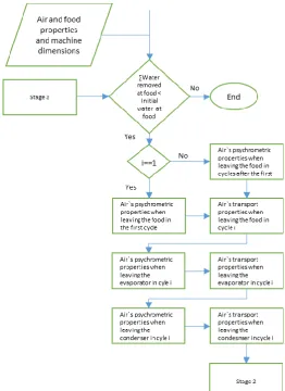
The algorithm can be represented in the form of a flow chart to illustrate the proposed logic map.
218
The first stage shown in Fig.2 results in the definition of the air`s psychrometric and transport
219
properties throughout the drying process, doing so from the Eq. (1) to (17) and the input data both
220
from the food and from the machine.
221
The first decision box of the flowchart present in this first stage is a part of the logical process of
222
the algorithm and should be included in any code as failsafe. The halting of the calculation process is
223
given when the variation of the moisture content over time reaches almost zero, 1E-9. This criterion
224
is flexible because it accommodates residual moisture differences from different types of food.
225
227
Figure 2. Stage 1 of the algorithm. The internal air analysis described in Eq. (1) to (17).
228
229
The properties outputs are used mainly as input for other stages. However, the program still can
230
provide this data to guarantee quality control, specifically through the monitoring of the air`s
231
temperature at the exit of each component.
232
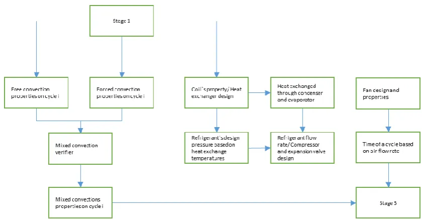
The second stage shown in Fig.3 outputs both design and process parameters. By taking the
233
aforementioned properties, it calculates the heat required to change the air`s state at both condenser
234
and evaporator. With it, and the expected enthalpy variation, the refrigerant mass flow rate is
235
achieved. These characteristics allow for an easy selection of the components required to design the
236
heat-pump of the dryer. These components are: compressor, expansion-valve, refrigerant fluid and
237
heat exchangers.
238
Even though the algorithm allows for easier selection of components, there are still some parts
239
that require manual selection. As commented in Section 2, the fans that circulate the air are
pre-240
selected to fit the drying container so that their dimensions are used as input data to calculate the
241
mass flow rate of the circulating air inside the machine.
242
244
Figure 3. Stage 2 of algorithm. Heat flow analysis between components, air and food.
245
Component design derived from Eq. (18) to (24).
246
247
For the final stage shown in Fig. 4, the results are given as a function of the amount of water in
248
the system. The algorithm outputs the rate of water removal. From it, the algorithm calculates how
249
this rate varies and how it effects the drying food. Finally, the variation of how much water is being
250
removed is used as a parameter for cycle control and break function.
251
252
253
Figure 4. Stage 3 of algorithm. Food humidity calculus and verification as demonstrated from
254
Eq. (25) to (33).
255
256
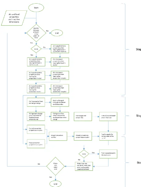
The whole algorithm is depicted in Fig. 5 showing the 3 stages that correspond, in Fig. 1, to the
257
259
Figure 5. Heat pump dryer design optimization algorithm
260
4. Discussion
261
The flow chart allows for an easier overview of the process (Fig. 5). This handy resource guides
262
its user from a basic starting point towards its desired goal which makes designing simpler since
263
The proposed algorithm is a tool of how to design the heat-pump air-based drier being also a
265
step-by-step guide. The value proposition is by providing the specifications of the components for
266
the machine that is going to be built (compressors, evaporators, condensers, etc.); and the fact that it
267
is not restricted by the food-drying physical models hereby proposed. The latter is a feature of the
268
algorithm because it is possible to update the used models of each process to the newest and most
269
sound ones available. Doing so, and using more accurate data, will impact the precision of the final
270
result. Actually, such a practice was used in the development of this algorithm. Data and equations
271
found in earlier versions of established guides and books such as [8] and [10] were posteriorly
272
replaced by newer ones [7].
273
The algorithm specifies each step and allows for the comprehension of the necessary and
274
produced data for that step. A code was written in GNU Octave automating the algorithm to deliver
275
as output a final value, and not clutter the user with processual information. In order to exemplify
276
the application of the code, one simulated the drying of the Agaricus Blazei mushroom for batches of
277
varying volumes that correspond to about 45, 123, 200, 277 and 355 kilograms of product. To simulate
278
the drying, and consequently provide suitable data for the design, it was considered the properties
279
pointed out by [5] related to the product`s fraction of water. Also, the input for stage 2 related to the
280
heat-exchangers and fan dimensions were based on the ECO coils and coolers of the Luvata Company.
281
282
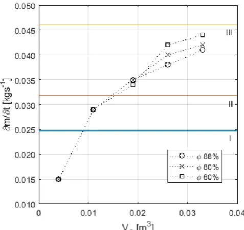
Figure 6. Relation of volume of product to required refrigerant flow.
283
284
Considering that 90% of the drying container`s volume is filled with food and that the
285
mushroom`s amount of water for 3 different cases is: 60%, 80% and 88%, the humidity removed can
286
be calculated based on the container’s volume. This is used as a variable parameter from which the
287
power output can be measured. Also, the temperature of drying was set to 80 °C, the superior
288
temperature limit from which this particular mushroom species starts having chemical and
289
organoleptic changes.
290
The algorithm simulated moisture removal for those given conditions and the results are
291
depicted in Fig. 6. The refrigerant mass flow rate is plotted against the volume of food in the drying
292
container, being a critical information for the selection of a suitable compressor. A commercial
293
compressor for nominal power operations yields a maximum mass flow rate. The graph represents
294
these working limits of 3 types of compressors from a given manufacturer (EMBRACO). The number
295
I, II and III respectively represent increasingly potent compressors of 610, 990 and 1445 W.
296
The simulation results show a clear need to upgrade the compressor from type I to II while
297
increasing the amount of Agaricus Blazei mushrooms from 45 to 123 kg, a 2.73-fold increase in drying
298
kg, will require a power increase of 1.46 times. The non-linearity of the drying process is clear, and
300
in this example, for the larger batches, from 200 to 355 kg, only one type of compressor would suffice.
301
For smaller batches the amount of humidity in the food is negligible for design purposes. For
302
larger batches the power needs are quite different. The dryer the food is, the harder the compressor
303
will have to work as it is depicted in Fig. 6. This is a known result and good indication of the proper
304
response of the algorithm.
305
The power needs for drying other types of products were also evaluated. Additional simulations
306
were done for fish from Thunnini tribe, comprising 15 species of the vulgarly known as tuna fish.
307
Because those species of fish (when fresh) are 3.3 times denser than mushrooms and have constant
308
moisture, more fish will fit into the drying chamber. There are also significant differences between
309
the experimental values of the drying curve from both products [15]. The experimental values for the
310
drying process are seldom available and changes may occur according to how the produce is
311
presented (whole, sliced, filleted, grinded, etc.). For example, a reduction of 1.57 times compressor
312
mass-flow rate (and the same amount in compressor power) is required when drying sliced fresh
313
tuna fish with a moisture content of 80% against the same volume of mushrooms. This contra intuitive
314
result derives from the fact that the drying temperature of the fish from Thunnini tribe cannot exceed
315
40 °C, thus a gentler drying is required. Different results may occur if the product is considered in a
316
different presentation, but the lack of public experimental drying curves is a caveat within this
317
industry.
318
5. Conclusions
319
A flexible optimization algorithm is presented, aimed to help design heat-pump air-based dryers
320
incorporating off-the-shelf components. The algorithm is segmented into 3 parts allowing the
321
modification or upgrade of any one according to new scientific developments. It also allows
322
dedicated solutions for different types and quantities of food because it incorporates their own
323
chemical and organoleptic limitations.
324
With this guide in hand, the selection of components and materials is simpler because the users
325
will have the key parameters of the required components and streamline the iterative process of
326
machine design.
327
The authors recommend that future versions of the algorithm, and possible programs,
328
incorporate more precise equations that consider the falling rate diffusion coefficient for the moisture,
329
possibly replacing Eq. (25) by a better one or using specific equations for different types of food.
330
331
332
Appendix A
333
List of variables and units.
334
𝑃𝑣𝑠 Vapor saturation pressure [pa]
335
𝑤 Absolute humidity [kg water/kg air]
336
𝑃𝑣 Air`s vapor pressure [pa]
337
𝐻 Enthalpy [kJ/kg*K]
338
∅ Relative humidity
339
𝑇𝑑𝑝 Dew point [K]
340
𝑣 Specific volume [m³/kg]
341
𝑋𝑣 Vapor molar fraction
342
k𝑎𝑟 Thermal conductivity of the humid air [W/m²*K]
343
𝑐𝑝 Specific heat [kJ/kg*K]
344
α Thermal diffusivity [m²/s]
𝜌 Mixture density [kg/m³]
346
𝜇𝑚𝑖𝑥 Dynamic viscosity [N*s/m²]
347
𝜏 Kinematic viscosity [m²/s]
348
∆𝑇𝑚𝑙 Logarithmic mean temperature difference [K]
349
𝑈 Mean global heat flux coefficient [W/m²*k]
350
𝑙 Thickness of the heat exchanger’s walls [m]
351
𝑘 Heat transfer coefficient of material [W/m²*K]
352
ℎ Convection heat transfer coefficient [W/m²*K]
353
𝑉 Air`s speed [m/s]
354
𝐴 Total exposed heat exchanger area [m²]
355
𝑚̇ or 𝜕𝑚𝜕𝑡 Mass flow rate [kg/s]
356
𝐷𝑎𝑏 Air diffusion coefficient [m²/s]
357
𝑚𝑙 Total water mass removed [kg/s]
358
𝑇 Absolute temperature [K]
359
𝐴𝑝 Plaque`s area [m²]
360
361
References
362
[1] M. Aktaş, L. Taşeri, S. Şevik, M. Gülcü, G. Uysal Seçkin, and E. C. Dolgun, “Heat pump drying of grape
363
pomace: Performance and product quality analysis,” Dry. Technol., vol. 0, no. 0, pp. 1–14, 2019.
364
[2] N. Malekjani and S. M. Jafari, “Simulation of food drying processes by Computational Fluid Dynamics
365
(CFD); recent advances and approaches,” Trends Food Sci. Technol., vol. 78, no. December 2017, pp. 206–
366
223, 2018.
367
[3] Á . Castell-Palou and S. Simal, “Heat pump drying kinetics of a pressed type cheese,” LWT - Food Sci.
368
Technol., vol. 44, no. 2, pp. 489–494, 2011.
369
[4] V. Demir, T. Gunhan, and A. K. Yagcioglu, “Mathematical modelling of convection drying of green table
370
olives,” Biosyst. Eng., vol. 98, no. 1, pp. 47–53, 2007.
371
[5] L. E. Kurozowa, “Efeito das condições de processo na cinética de secagem de cogumelo,” p. 121, 2005.
372
[6] R. P. Lopes, D. C. Lopes, and R. C. Rezende, Secagem e Armazenagem de Produtos Agrícolas. Aprenda Fácil
373
Editora ISBN 978-85-62032-00-4, 2008.
374
[7] P. T. Tsilingiris, “Thermophysical and transport properties of humid air at temperature range between
375
0 and 100 °C,” Energy Convers. Manag., vol. 49, no. 5, pp. 1098–1110, 2008.
376
[8] A. S. of H. R. and A. C. Engineer, 2015 ASHRAE HANDBOOK Inch-Pound Edition. 2015.
377
[9] N. Yamankaradeniz, K. F. Sokmen, S. Coskun, O. Kaynakli, and B. Pastakkaya, “Performance analysis
378
of a re-circulating heat pump dryer,” Therm. Sci., vol. 20, no. 1, pp. 267–277, 2016.
379
[10] F. P. Incropera and F. P. Incropera, Fundamentals of heat and mass transfer., 6th ed. John Wiley, 2007.
380
[11] Y. A. M. A. B. Cengel, Thermodynamcis, An Engineering Approach, 8th ed. Mc Graw-Hill Interamericana,
381
2007.
382
[12] L. J. Goh, M. Y. Othman, S. Mat, H. Ruslan, and K. Sopian, “Review of heat pump systems for drying
383
application,” Renew. Sustain. Energy Rev., vol. 15, no. 9, pp. 4788–4796, 2011.
384
[13] C. O. Perera and M. S. Rahman, “Heat pump dehumidifier drying of food,” Trends Food Sci. Technol., vol.
385
[14] M. T. . and M. E.A., “Gaseous Diffusion Coefficients,” J. Phys. Chem., vol. 118, 1972.
387
[15] U. U. Modibbo, S. A. Osemeahon, M. H. Shagal, and M. Halilu, “Effect of Moisture content on the drying
388
rate using traditional open sun and shade drying of fish from Njuwa Lake in North- Eastern Nigeria,”