The Development of a New
Lightning-Frequency
Parameterization and its
Implementation in a Weather
Prediction Model
Dissertation
Fakult¨at f¨
ur Physik
Ludwig-Maximilians-Universit¨at
M¨
unchen
Dipl.-Met. Johannes M. L. Dahl,
Berlin
Gutachter der Dissertation:
1. Gutachter: apl. Prof. Dr. U. Schumann 2. Gutachter: Prof. Dr. G. C. Craig
Contents
Contents i
Zusammenfassung 1
Abstract 3
1 Introduction 5
1.1 Thesis goals and outline . . . 7
2 Background 9 2.1 Thunderstorm structures . . . 9
2.1.1 Deep moist convection . . . 9
2.1.2 Organization of convection . . . 10
2.2 Charging mechanisms of thunderclouds . . . 12
2.3 Lightning . . . 14
2.3.1 Lightning detection with LINET . . . 14
2.3.2 Lightning initiation and lightning types . . . 15
2.3.3 Definition of a “flash” . . . 17
2.4 The flash rate . . . 18
2.4.1 General considerations . . . 18
2.4.2 Application to a two-plate capacitor . . . 20
2.4.3 Assumptions and their limitations . . . 22
2.4.4 Interpretation of the flash-rate equation . . . 24
2.5 Single-parameter approaches . . . 26
2.5.1 Popular single-parameter approaches and their limitations . . 26
2.5.2 Flash rate and generator power . . . 30
2.5.3 The Grewe et al. (GR01) parameterization . . . 32
3 The New Lightning-Frequency Parameterization 37 3.1 Parameterizations . . . 37
3.1.1 Area of the capacitor plates . . . 38
3.1.2 The lightning efficiency, γ . . . 39
ii CONTENTS
3.1.3 Lightning charge and generator-current density . . . 39
3.2 Definition of a cell in the PR92, YMUK09, and GR01 approaches . . 44
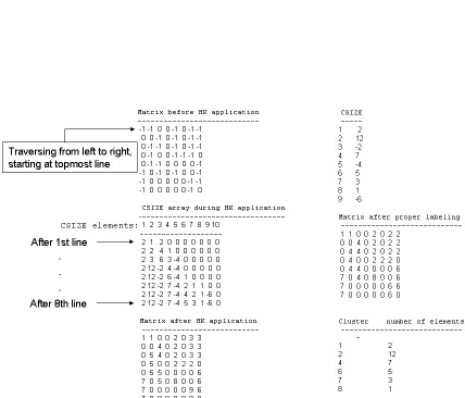
4 Implementation 49 4.1 Description of the algorithm . . . 49
4.2 Implementation of the algorithm . . . 52
4.2.1 Source-code organization . . . 52
4.2.2 The module src lightning.f90 . . . 53
4.2.3 Input and output . . . 57
4.3 COSMO-DE-specific additions . . . 58
4.4 Other parameterizations . . . 59
5 Tests of the New Lightning Parameterization 61 5.1 Individual observed cumulonimbus clouds . . . 61
5.2 Environmental parameters . . . 74
6 Application 77 6.1 Application to individual simulated cumulonimbus clouds . . . 77
6.1.1 22 August 2008 . . . 79
6.1.2 2 April 2008 . . . 79
6.1.3 5 July 2009 . . . 80
6.1.4 1 March 2008 . . . 81
6.1.5 26 May 2009 . . . 82
6.2 Observed and simulated lightning over southern Germany . . . 83
6.2.1 22 August 2008 . . . 83
6.2.2 5 July 2009 . . . 89
7 Discussion 103 7.1 Lightning data . . . 103
7.2 The D10 approach . . . 104
7.3 The PR92, YMUK09, and GR01 approaches . . . 107
7.4 D10 application: individual cells in COSMO-DE . . . 110
7.5 COSMO-DE implementation - entire domain . . . 111
7.6 Sounding-derived parameters . . . 115
8 Conclusions and Outlook 117 8.1 Future work . . . 120
CONTENTS iii
A.3 The charging current . . . 126 A.4 The generator power . . . 128
B The COSMO-DE Model 131
C List of Abbreviations and Symbols 133
Bibliography 139
Acknowledgments 147
Zusammenfassung
Basierend auf einem einfachen physikalischen Modell wurde eine neue Blitz-Parametrisierung entwickelt. Hierbei repr¨asentiert ein Plattenkondensator die grundlegende Dipol-Ladungsstruktur einer Gewitterwolke. Dieser Kondensator wird kontinuierlich durch einen Generator-Strom aufgeladen und durch Blitzentladungen entladen. In dem hier verfolgten Ansatz werden der Generatorstrom sowie die St¨arke der Entladungen mithilfe des Graupelmasse-Feldes parametrisiert. Aus diesen bei-den Gr¨oßen kann die Blitzfrequenz eindeutig bestimmt werbei-den, wenn sich Generator-und Entladungs-Strom im Gleichgewicht befinden. Mit diesem Ansatz k¨onnen Un-zul¨anglichkeiten fr¨uherer theoretischer ¨Uberlegungen, bei der die Blitzrate beispiel-sweise mit der Leistung des Gewitters in Verbindung gesetzt wird, behoben werden. Um diesen Ansatz zu testen, wurden polarimetrische Doppler-Radar-Daten be-nutzt, mittels derer die Graupelverteilung in beobachteten Gewittern ermittelt wer-den konnte. Die Blitz-Aktivit¨at wurde mithilfe des LINET-Netzwerks bestimmt. Der Vergleich zwischen theoretisch vorhergesagten und beobachteten Blitzraten ist ermutigend: F¨ur isolierte Gewitterzellen liefert der theoretische Ansatz genaue Ergebnisse. Zwei bereits existierende Parametrisierungen, in denen die vertikale Wolkenm¨achtigkeit zur Beschreibung der Blitzrate verwendet wird, zeigen deutlich weniger G¨ute.
Diese beiden existierenden Ans¨atze, der im Kontext dieser Arbeit neu entwick-elte Ansatz sowie ein weiterer, welcher auf der Vertikalgeschwindigkeit im Aufwind des Gewitters beruht, wurden in das Wettervorhersagemodell COSMO-DE imple-mentiert. Mit diesem Modell wurden reale Gewitter-Szenarios simuliert. Die G¨ute der Parametrisierungen anhand modellierter Konvektion zu testen ist schwierig, da es generell keine eindeutige Zuordnung zwischen beobachteten und modellierten konvektiven Wolken gibt. F¨ur F¨alle, in denen ein direkter Vergleich zwischen simulierten und beobachteten Gewitterzellen m¨oglich war, waren die Ergebnisse ebenfalls vielversprechend. Ein Vergleich der gesamten Blitzaktivit¨at in einem Ge-biet, das v.a. den S¨uden Deutschlands beinhaltet, zeigt, dass keiner der implemen-tierten Ans¨atze die Blitzaktivit¨at zufriedenstellend widerspiegelt. Dies ist v.a. darin begr¨undet, dass im COSMO-DE die Gewitterzellen nicht in der korrekten Anzahl und zur korrekten Zeit entstehen.
Abstract
Based on a straightforward physical model, a new lightning parameterization has been developed: A two-plate capacitor represents the basic dipole charge structure of a thunderstorm, which is charged by the generator current and discharged by lightning. In this approach, the generator current as well as the discharge strength are parameterized using the graupel-mass field. If these two quantities are known, and if the charging and discharging are in equilibrium, then the flash rate is uniquely determined. This approach remedies shortcomings of earlier theoretical approaches that relate the flash rate e.g., to generator power. No distinction is made between intracloud and cloud-to-ground discharges.
In order to test this approach, polarimetric radar data were used, from which the graupel distribution in observed thunderstorms could be inferred. The light-ning activity was detected using the LINET network. The comparison between theoretically-predicted and measured flash rates is encouraging: Over a wide range of flash rates, the theoretical approach yields accurate results for isolated thunder-storms. Two existing parameterizations, which only use the depth of the clouds as predictor, produce substantially less accurate forecasts.
These two existing approaches, the one developed in this study, as well as a fourth one based on updraft velocity, were implemented in the convection-resolving COSMO-DE numerical weather prediction model. With this model, real-world con-vective scenarios were simulated. The output of the lightning scheme includes the location and time of every simulated discharge. Testing the performance of the parameterizations with modeled convection is difficult as there is no one-to-one cor-respondence between observed and modeled convective clouds. Where a comparison between modeled and observed flash rates of individual clouds was possible, the results for individual cells were promising.
The comparison of the bulk lightning activity over an area comprising southern Germany and adjacent countries suggests that none of the four parameterizations captures the overall lightning activity well. This is mainly because COSMO-DE does not simulate the observed number of cells at the correct times.
Chapter 1
Introduction
Atmospheric lightning is associated with a variety of meteorological and geophys-ical phenomena, deep moist convection arguably being the most common among these. Besides, lightning is known to accompany volcanic ash plumes and dust storms (Uman, 2001, p. 26), and it may even be associated with piezoelectric ef-fects preceding earthquakes (Finkelstein and Powell, 1970). However, these types of lightning shall not be the subject of this study, but only those that are associated with thunderstorms. Given the spectacular visual and acoustic manifestation of thunderstorm discharges, as well as the threat to life and property posed by them, they have always fascinated mankind and they have been a persisting subject of research efforts.
With the advent of numerical models, deep convective clouds could be simu-lated (Klemp and Wilhelmson, 1978) and soon electrification models were included. In 1982, Rawlins (1982) first considered charging and discharging processes but no lightning channels yet. Helsdon and Farley (1987) simulated channel propagation us-ing a two-dimensional model. Nowadays, advanced three-dimensional cloud models are equipped with sophisticated electrification schemes (e.g., Mansell, 2000; Mac-Gorman et al., 2001; Barthe et al., 2005). These make use of the results from labora-tory experiments (e.g., Takahashi, 1978; Jayaratne, 1998; Saunders and Peck, 1998), which determine the magnitude and direction of charge transfers during hydrome-teor collisions. Dielectric breakdown is modeled explicitely by initiating lightning channels which exhibit realistic branching and propagation (Mansell, 2000).
These parameterizations were implemented in cloud models and more recently in convection-resolving mesoscale models (Barthe et al., 2005).
A sophisticated analytical model involving a basic dipole charge structure was developed by Driscoll et al. (1992). In their model, the generator current, the lightning current, and other parameters need to be prescribed to determine the average current towards the ionosphere.
Another approach was stimulated by Vonnegut (1963), who suggested that the
6 Introduction
electrical power of a storm can be determined if the flash rate and the flash energy are known. This idea was further developed by Williams (1985) who proposed that the flash rate varies linearly with storm power. After several assumptions mainly about storm geometry, he found that the lightning rate varies as the 5th power of
the cloud-top height. This result was condensed into a separate parameterization by Price and Rind (1992). Similarly, the lightning frequency has been linearly related to the charging current (Blyth et al., 2001; Deierling et al., 2008; Yoshida et al., 2009). Other investigators have found correlations between the lightning rate and the convective rainfall rate (e.g., Ch´eze and Sauvageot, 1997; Tapia et al., 1998). In their essence, all these are “single-parameter” approaches as they relate the flash rate to a single predictor.
These approaches only consider the charging of the cloud while making implicit and partly unphysical assumptions about the neutralization of the charge during a lightning flash. By employing a straightforward physical model in this study, this shortcoming is remedied. This model involves a two-plate capacitor which is applied to convective clouds. Since the charging is parameterized by merely considering the graupel-mass field, this model is less sophisticated than those by Barthe et al. (2005) and Mansell (2000). Also, the lightning channels are not explicitly modeled and only the instantaneous lightning rate is determined. Moreover, no distinction is made between cloud-to-ground and intra-cloud discharges. However, the location and time of each flash are determined, so that an accurate display of the simulated flashes is possible, directly comparable to measurements by lightning-detection net-works. As such, the underlying physical model as well as the products yielded by the lightning scheme, may be considered to be a compromise between the highly sophisticated approaches and the single-parameter approaches. The latter ones are usually implemented such that a flash-rate value is depicted for each gridbox (e.g., Price and Rind, 1992). These approaches were intended mostly for applications on the global scale (Price and Rind, 1992; Tost et al., 2007; Yoshida et al., 2009) and the highly-sophisticated schemes are mostly used either in cloud models or in ideal-ized studies with convection-resolving mesoscale models. Since the main application of the scheme developed herein is real-world scenarios, the intermediate degree of sophistication seems to be an appropriate choice.
1.1 Thesis goals and outline 7
(in convection-resolving models, there is no distinction between convective and non-convective precipitation; thus the accumulated precipitation field would not provide such a clear picture).
Lightning plays an important role in atmospheric chemistry. Chemical reac-tions in the lightning channel result in the creation of nitrogen oxides, NOx
(Schu-mann and Huntrieser, 2007; Grewe, 2009; Pickering et al., 2009). Schu(Schu-mann and Huntrieser (2007) estimate the total equivalent mass of lightning-produced NOx to
be 5 ± 3 Tg per year. Lightning NOx (often referred to as LNOx) affects the
free-atmospheric ozone production, which in turn acts as greenhouse gas. LNOx may
thus be considered as indirect greenhouse gas, and its emission is an important factor in climate-change scenarios.
The simulations may also provide insight into the thermodynamic and kinematic environments of thunderstorms in relation to their electrical activity. Apart from that, there has been a long discussion about the processes that govern the flash rate (e.g., Boccippio, 2002; Yoshida et al., 2009). With the straightforward approach pursued in this work, some of these question could be answered (e.g., is the flash rate proportional to the electric power that the storm generates, or to the charging current?).
1.1
Thesis goals and outline
The specific goals of this study are to
• develop a new method to diagnose the flash rate in a thunderstorm cloud,
• implement this method in the COSMO-DE model,
• implement three existing parameterizations in COSMO-DE,
• test the new method with observed thunderstorm clouds and compare the predictions with results from existing parameterizations,
• apply all parameterizations to simulations of real-world scenarios,
• compare the simulation results based on the different parameterizations.
8 Introduction
of the test and the simulations will be discussed in chapter 7. A summary and suggestions for future work are offered in chapter 8.
Chapter 2
Background
2.1
Thunderstorm structures
A thunderstorm is a complex phenomenon, which involves updrafts, downdrafts, and precipitation processes which are all interacting with each other. Arguably, the heart of a thunderstorm is its updraft: Hydrometeor and downdraft formation, as well as all other processes accompanying a thunderstorm are secondary effects which would not occur if no updraft had existed previously. Hence, this section will focus on the physics of deep, free convective updrafts.
2.1.1
Deep moist convection
The necessary, albeit not sufficient condition for such a moist buoyant updraft to arise, is the existence of conditional instability and moisture. These may be com-bined in a single quantity, theconvective available potential energy (CAPE). CAPE is the potential energy of a parcel due to thermal buoyancy,
CAPE =R
Z p(z1)
p(z2)
Tv
′
d(lnp), (2.1)
where R is the individual gas constant of dry air, Tv
′
is the virtual temperature perturbation due to the parcel, p is pressure, and the heights z1 and z2 bound the region where free ascent occurs.
Usually, the air parcels making up the convective cell have to be lifted somewhat before becoming positively buoyant. This stable region is characterized by the con-vective inhibition, CIN, which is the energy required to overcome this layer. The level at which the free ascent commences is referred to as level of free convection (LFC). The level where the parcel’s temperature equals the environmental temperature, is calledequilibrium level (EL). It follows, that for a deep, moist convective updraft to develop, conditional instability, moisture, and lift need to coincide (Doswell, 1987;
10 Background
Johns and Doswell, 1992). An example of a sounding with positive CAPE is shown in Fig. 2.1.
2.1.2
Organization of convection
Once a convective updraft has formed, precipitation particles develop and fall through the updraft, which gradually weakens and eventually completely dimin-ishes as a consequence. The life cycle of such a convective system was categorized into three stages, i.e., the cumulus stage, the maturity stage, and the dissipation stage by Byers and Braham (1949). These authors defined the maturity stage to commence as precipitation begins reaching the ground. In the dissipation stage, merely the cool, precipitation-laden downdraft is left. The time scale of this entire process is on the order of 30 min. Though rarely met in nature, this single-cellular form of storm structure represents the archetype of a weakly-organized convective system.
At the other end of the spectrum, there are well-organized, long-lived and often quite severe thunderstorms. A key to storm organization is vertical wind shear. There are at least three reasons that wind shear is supportive of storm organiza-tion: i) Updrafts and downdrafts become laterally separated, reducing the demise of the updrafts as precipitation forms and falls within them (e.g., Houze, 1993); ii) a vertically-sheared flow contains horizontal vorticity, which may be tilted into the vertical by updrafts (e.g., Davies-Jones, 1984), and rotation of the thunderstorm cell may ensue. In many circumstances, this vorticity is thought to reduce the turbulent energy cascade within the updraft, and hence increase its longevity and strength (e.g., Lilly, 1986); iii) a non-hydrostatic pressure field develops in and around up-drafts in sheared environments (Rotunno and Klemp, 1982; Davies-Jones, 2002). A dramatic example of a storm in strong shear is the supercell (Rotunno, 1993; Doswell and Burgess, 1993), which possesses a long-lived, rotating updraft, and whose dy-namics is dominated by dynamic perturbation pressure gradient forces (Rotunno, 1993). An example of a supercell storm is shown in Fig. 2.2. The reflectivity as well as the doppler velocity fields are shown, nicely displaying the supercell’s hook echo as well as the mesocyclonic circulation.
The dynamics of linearly-organized storms, like squall lines, is dominated by the pressure field that develops in and around the precipitation-generated cold pool (Trapp and Weisman, 2003; Weisman, 2001; Weisman et al., 1988). Though the gustfront also plays a role in supercell dynamics, a supercell can be sustained in the absence of gustfronts1, while squall lines cannot.
This spectrum is continuous, with structures like squall lines and supercells
1
2.1 Thunderstorm structures 11
Figure 2.1: Skew T-log p diagram from M¨unchen-Oberschleissheim on 23 June 2008, 12 UTC. Wind barbs: pennant = 25 ms−1
; long barb = 5 ms−1
; short barb = 2.5 ms−1
. The list on the right shows several convective parameters, including the virtual-temperature corrected mixed-layer CAPE (CAPV) and the corresponding CIN value (CINV). The sampled air mass is minimally capped (CINV = -0.79 J kg−1
), rather unstable (CAPV = 1,445 J kg−1
) and strongly sheared (about 40 knots (≈ 20 ms−1
12 Background
placed at the well-organized end, and the short-lived single cell at the weakly-organized end of the spectrum. Multicellular storms that share a common gust-front and that are organized in the mesoscale are referred to asmesoscale convective system (MCS) (NCAR, 1984). The most prominent type of MCS is a squall line.
Filename: /data/radar/HP/Y2008/M06/D23/ST008/SCAN0009.gz Date & Time: Mon Jun 23 12:37:54 2008
Product: PPI-TXX Elevation: 1.0 deg
Scan-Type: Type 4711 - PRF: 1150 Hz dBZ 60.00 56.33 52.65 48.97 45.30 41.62 37.95 34.28 30.60 26.92 23.25 19.58 15.90 12.23 8.55 4.88 1.20 -2.47 -6.15 -10.00 (a) Filename: /data/radar/HP/Y2008/M06/D23/ST008/SCAN0009.gz Date & Time: Mon Jun 23 12:37:54 2008
Product: PPI-VYY Elevation: 1.0 deg
Scan-Type: Type 4711 - PRF: 1150 Hz m/s 16.00 14.32 12.64 10.96 9.28 7.60 5.92 4.24 2.56 0.88 -0.80 -2.48 -4.16 -5.84 -7.52 -9.20 -10.88 -12.56 -14.24 -16.00 (b)
Figure 2.2: POLDIRAD PPI images of a supercell on 23 June 2008. (a) shows the reflectivity field, displaying a well-pronounced hook echo (appendage to the southwest of the main echo). (b) shows the radial-velocity signature of a mesocyclone where the hook echo is located.
2.2
Charging mechanisms of thunderclouds
Non-inductive charging The basic charging process is believed to occur during collisions between graupel pellets with ice crystals and subsequent sedimentation that results from the different terminal fall velocities of both hydrometeor classes (e.g., Takahashi, 1978). The underlying theory is called relative growth rate (RGR) theory (Baker et al., 1987): Charge transfer during hydrometeor collisions proceeds according to the following rule: Of two colliding particles, the one with the larger depositional growth rate charges positively due to the loss of negative charge. The one with the lower depositional growth rate charges negatively (Dash et al., 2001; Saunders, 2008). The reason for the surface charge is the formation of an electric double layer which forms as a result of ion defects in the lattice structure during depositional growth. The stronger this growth, the more surface charge accumulates. The ion defects are associated with broken bonds of the H2O molecules. As the H+
ions are rather mobile, they diffuse towards the interior of the particle while the OH−
latent-2.2 Charging mechanisms of thunderclouds 13
heat release. This may locally increase the degree of ice supersaturation.
Transferring this rule to a natural deep convective cloud, the result is a selec-tive charge transfer between riming graupel pellets and ice crystals. This charge transfer changes sign at a certain temperature, the so-calledcharge-reversal temper-ature. The typical configuration of a natural deep convective cloud is such that the graupel attains negative charge roughly above the 263 K level (and the ice crystals gain positive charge), i.e., there is a transfer of negative charge from the ice crystals to the graupel pellets. Below this level, the charge transfer is opposite, and grau-pel charges positively (e.g., Saunders, 2008). Subsequent sedimentation allows for accumulation of space charge within the cloud. A basic electric “tripole” structure of a thunderstorm hence results, with a main positively charged region in the upper portions of the storm where ice crystals dominate, and a main negatively charged region somewhat above the 263 K isotherm where graupel dominates. A weaker positively charged region exists in the lower portions of the cloud (Williams, 1989). The cause of this charge region is not fully agreed upon. Aside from the graupel-ice collisions, possible mechanisms are ion capture, charge deposited by lightning, and inductive charging (Williams, 1989; Mansell, 2000). To gain insight into the hy-drometeor distribution in a real-world cloud, Fig. 2.3 shows the hyhy-drometeor classes derived from polarimetric radar data (H¨oller et al., 1994).
14 Background
Inductive charging The inductive charging mechanism requires a strong pre-existing electric field which results in a polarization of the hydrometeors. That is, inductive charging is considered to be a secondary effect after appreciable field strength has been achieved by the non-inductive charging process. The only viable collision partners are thought be cloud droplets and graupel particles (Saunders, 2008; Mansell, 2000). Other particles may coalesce or exhibit too weak a polarization for charge transfer to occur.
Convective charging Grenet and Vonnegut suggested that positive fair-weather charge is ingested into the updraft, which results in a negative screening-layer charge (e.g., MacGorman and Rust, 1998). In this theory, the screening-layer charge is advected into the interior of the storm as descending motion at the updraft’s flanks occurs. This hypothesis falls short of explaining observed charge structures and has largely been dismissed as initial electrification mechanism. However, it does have relevance in that it emphasizes the importance of convective motions that may re-distribute charge that has previously been isolated by other processes (MacGorman and Rust, 1998).
The above-mentioned tripole structure of a convective storm is a strong over-simplification. Even in the simplest setup, there are at least four charge layers, as a region of negative screening-layer charge forms at the top cloud boundary owing to ion attraction. As soon as the storm becomes organized, e.g., into an MCS with an extensive precipitation region behind or ahead of the convective line, multiple charge layers have been observed (Stolzenburg et al., 1998). Also, supercells where the main positive dipole was inverted have been observed, which may be explainable with unusual effective liquid water contents in the context of the RGR-hypothesis (Rust et al., 2005). Fig. 2.4 sketches the gross charge structure of a thunderstorm.
2.3
Lightning
2.3.1
Lightning detection with LINET
2.3 Lightning 15
Figure 2.4: This sketch shows a convective cell and its basic charge structure, including screening-layer charge. Plus signs denote positive charge, minus signs denote negative charge.
process close to the ground, while radiation from IC-discharges originates at higher altitudes (Betz et al., 2009). This height of the discharge is also determined by the TOA technique, making any assumptions about wave forms that may belong to either intra-cloud or cloud-to-ground discharges unnecessary. The location accuracy is on the order of 100 m based on measurements on towers whose positions are well known.
2.3.2
Lightning initiation and lightning types
The details about streamer initiation and subsequent leader formation remain elu-sive, the main issue being that the electric-field strength necessary for field break-down has never been observed in thunderclouds (e.g., Solomon et al., 2001). A possible explanation is that local field enhancements at the edges of hydrometeors allow for positive streamer initiation. Once a streamer system has developed, the field at the streamer origin increases beyond the critical field strength for break-down. However, this process still requires fields higher than what has been observed (Petersen et al., 2008). Although it is possible that compact regions of enhanced field strength simply have not been sampled, evidence is accumulating that the ex-istence of the conventional breakdown field strength of air is not necessary. Rather, high-energy seed electrons due to a cosmic-ray shower may trigger a so-called run-away breakdown (Gurevich et al., 1992; Marshall et al., 1995). The required field strength, called “breakeven” field strength, is an order of magnitude smaller than the conventional breakdown field strength (about 100 kV m−1
vs 1,000 kV m−1
16 Background
0 20 40 60 80 100 120 140 160 180 -1000
-500 0 500 1000
17:05:38.2468289
d
.u
.
t [ ms ]
1 2 3 4 5 6..10 11 12 131415 16
Figure 2.5: LINET measurements showing K-changes during an IC discharge. Only the highlighted pulses are reported by the system. Adapted from Schmidt (2007).
result in polarized plasma which enhances the electric field at its tips. This field enhancement could then initiate positive streamers from nearby hydrometeors. Pe-tersen et al. (2008) suggest that a combination of both processes may occur. In any case, once a system of cool plasma streamers has developed, these are thought to combine into a hot and highly conductive leader channel (Petersen et al., 2008).
2.3 Lightning 17
Cloud-to-ground (CG) lightning It has been shown that in general the leader develops amidst the largest potential gradients between the space-charge regions and propagates into potential wells (Coleman et al., 2003). During a negative cloud-to-ground discharge (-CG), a bidirectional leader usually forms between the main negative charge and the lower positive charge regions. Usually, the negative leader propagates horizontally through the lower positive charge region during preliminary breakdown (Stolzenburg and Marshall, 2009). Once the leader reaches the ground, one or more upward connecting leaders are initiated from the surface. This attach-ment process short-cuts the circuit and allows the negative charge in the leader channel to be drained to the surface. This main, upward propagating discharge is known as return stroke. Once the charge is removed from the channel, a junc-tion process (J-process) usually occurs, which involves recoil-leader discharges. This leads to the initiation of a second leader, the dart-leader, which usually retraces the residual channel of the previous discharge. Once this leader has attached to the ground, a subsequent return stroke may occur. This process may be repeated sev-eral times, so that most flashes exhibit sevsev-eral return strokes. Sometimes, a rather long-duration discharge (hundreds of milliseconds) follows the last return stroke, the so-called continuing current, which taps charge from the cloud, rather than the charge deposited in the channel. Only the return-stroke components of the CG discharge can be detected with LINET.
For more details about lightning discharges, see, e.g., Petersen et al. (2008), Stolzenburg and Marshall (2009), Ogawa (1995), or Rakov and Uman (2003).
2.3.3
Definition of a “flash”
The foregoing discussion implies that there is no single, well-defined discharge pro-cess. Rather, the discharge is a complicated, multi-stage phenomenon, involving electrical currents within multiple time and length scales. For the present purpose, a practical definition of a “discharge event” (= “flash”) was needed:
A flash includes all single discharges reported by LINET (called “stroke” independent of lightning type) that occur within one second and within a
radius of 10 km.
18 Background
distribution of strokes. An impractical but more accurate method would be to select a radius that includes the convective system under consideration. However, a 10 km radius seems to be a reasonable compromise for most central-European storms. The advantage of such binning is that variations in detection efficiency are filtered out. The flash measurements thus are more robust to changes in the antenna coverage than stroke measurements. Also, in most studies flashes are considered rather than strokes, and to compare the results obtained in this study with other results, group-ing the strokes into flashes seemed to be appropriate. Fig. 2.6 shows an example of the dependence of the flash number on the choice of the space and time intervals. As can be seen, the total number of flashes is quite strongly dependent upon the choice of the radius and time intervals.
(a) (b)
Figure 2.6: (a) Dependence of the number of accumulated flashes on the selected time interval at a radius of 10 km. (b) Dependence of the number of flashes on the selected radius at a time interval of 1 s. The abscissa is scaled to 1,000 flashes to improve readability. The number of accumulated strokes on 26 May 2009 was 280,614.
2.4
The flash rate
In this section, a theoretical framework is provided which yields a general expression for the flash rate based on a simple capacitor model.
2.4.1
General considerations
2.4 The flash rate 19
The time,T, for this initial charging is related to the rate at which the vertical component of the electric field,E, increases and to the critical electric field strength,
Ec:
Ec =
Z T
0 ∂E
∂t dt. (2.2)
At the time, T, the critical field strength is reached, and a discharge occurs. The strength of the discharge, i.e., the amount of charge transferred, determines the degree to which the electrostatic field has been neutralized. This is just the field strength that needs to be replenished before the next flash can occur. If ¯E is the field strength after the discharge, the field strength that needs to be restored is given by
Ec−E¯ = ∆E =τ
∂E
∂t , (2.3)
where ∆E is the field strength that needs to be replenished for the next discharge to occur, and τ is the time required to rebuild the field. The charging rate, ∂tE,
has been assumed to be constant between two discharges. The discharge rate,f, is then given by
f = 1
τ =
1 ∆E
∂E
∂t . (2.4)
This equation may be re-written as
∂E
∂t −f∆E = 0, (2.5)
20 Background
Now ∆Emay be expressed with the aid of a so-calledneutralization efficiency2, η, so that
∆E =ηEc, (2.6)
where
η= Ec −E¯
Ec
. (2.7)
Hence, the discharge rate is given by
f = 1
ηEc
∂E
∂t . (2.8)
Obviously, the larger η, i.e., the stronger the discharge, the larger the electrostatic field that needs to be restored before the next flash can occur, and the smaller the flash frequency. E.g.,η = 1 implies that the entire field has been neutralized during the discharge.
Instead of the electrostatic field, any other quantity may be chosen that uniquely describes when breakdown takes place. Apart from the electrostatic field, this could be the charge or the charge density. If this general quantity is denoted with Ψ, then the flash-rate equation may be written as
f = 1 ∆Ψ
∂Ψ
∂t . (2.9)
Eq. (2.5) then takes the form
∂Ψ
∂t −f∆Ψ = 0. (2.10)
2.4.2
Application to a two-plate capacitor
To obtain quantitative results, specification of the space-charge distribution is neces-sary. In the following paragraphs, an analytical solution of Gauss’ law for a two-plate circular capacitor will be used as basis for the new lightning-frequency parameteri-zation. Fig. 2.7 summarizes the charge geometry. The lightning current, IL (shown
in yellow), is given by
IL= ∆Qf, (2.11)
i.e., the product of lightning rate, f, and lightning charge, ∆Q. This current is balanced by the generator current (black arrows in Fig. 2.7). This balance between
2
2.4 The flash rate 21
Figure 2.7: Sketch of the capacitor used to model the space-charge regions of a thunder-storm. The geometric parameters, R and d, are shown, as well as the lightning current (yellow, lightning-shaped arrows) and the generator current (black arrows). Plus and minus signs refer to the sign of the plate charge.
charging current and lightning current is consistent with Eq. (2.10), which simplifies to
Ic −IL= 0, (2.12)
where the charge, Qwas inserted for Ψ. The charging current, Ic, is given by ∂tQ.
This means that if the charging current is known, then the lightning current is known as well. In order to infer the flash rate, only the lightning charge needs to be prescribed (this will be done in the next chapter). Assuming positive charge on the upper capacitor plate and negative charge on the lower capacitor plate, the electric field in the center of the capacitor and in the middle of the plates is given by (see Appendix A.1 for a detailed derivation):
E(R, d) =−σ
ǫ + σ
2ǫ
d
q
R2+ (d
2)2
, (2.13)
22 Background
Differentiating Eq. (2.13) with respect to time yields
∂E ∂t =
j
2ǫ[G(R, d)−2], (2.14)
where
G(R, d) = q d
R2+ (d
2)2
(2.15)
is the geometric term, which depends on the radius of the plates and their separation distance. This expression is valid only in the center of the capacitor between the plates where lightning initiation usually occurs (see Stolzenburg and Marshall, 2009, and also Appendix A.1). Upon inserting Eq. (2.14) into the flash-rate equation,
f = 1 ∆E
∂E
∂t , (2.16)
one obtains for the lightning frequency
f = 1 2ǫ
j
∆E(G(R, d)−2). (2.17)
2.4.3
Assumptions and their limitations
Two charge regions
An obvious simplification is that the model features only two charge regions. How-ever, it is generally agreed upon that the main positive dipole represents the gross charge structure of thunderstorms (MacGorman and Rust, 2008, p. 50), with ad-ditional charge regions having smaller magnitudes. Though these may be crucial for the details of the electric activity of thunderstorms, it is suggested in this study that the gross electric behavior is described already if only two charge regions are assumed. This simple assumption is not expected to hold if large thunderstorm systems (rather than isolated cells) are considered, because such systems exhibit substantially more complicated charge distributions (Stolzenburg et al., 1998).
Equal size of charged regions
2.4 The flash rate 23
indicate a rather complicated charge structure in the anvil (e.g., Mansell, 2000). The degree of inaccuracy resulting from the choice of equal plate size is thus not larger than assuming a radially-symmetric charge-density decay. In this implementation, the choice was made in favor of the easier solution.
Qualitatively, this choice has two effects: The total critical charge is reduced compared to the case where the upper plate is bigger than the lower plate. This effect implies an increased lightning rate, because the relative reduction of space charge decreases with increasing plate geometry (Fig. 2.8(b)). The other effect is that an increased size of the space-charge region increases the lightning charge, which contributes to a reduced flash rate. Though these two effects may cancel one another, this cannot be quantified based on the current state of knowledge.
Circular plates
The assumption that the horizontal cross-section through a deep convective cloud is circular, is a first-order approximation. One may consider the actual (usually, non-circular) charge distribution as being composed of a circular contribution and a departure thereof. The main effect of this perturbation from the circular base-state configuration is that boundary effects gain dominance (these contributions increase as the perturbation increases). To quantify these effects, the numerical solution of Gauss’ law for arbitrary plate shapes may be compared to the analytical circular-plate solution. In general, the deviation from the circular-circular-plate solution will vary from storm to storm, depending on the departure from a circular charge distribution. The fact that an analytical solution exists for the electrostatic potential around cir-cular plates (Appendix A.1) was the main reason for assuming this charge geometry. Moreover, convective updrafts are often successfully modeled as horizontally circular objects (e.g., Davies-Jones, 2002).
The radius of the circular area equivalent is given by
R =
r
A
π, (2.18)
where A is the horizontal cross-sectional area of the graupel region through its vertical centroid location.
Though not required to determine the flash rate, the vertical separation distance of the plates is also determined as part of the model output (see p. 58 for more details). The separation distance is given by the distance between the centroid positions of the two space-charge regions.
24 Background
of the space-charge regions. This thickness, multiplied with the plate area is the assumed charge-region volume.
2.4.4
Interpretation of the flash-rate equation
Equation (2.17) is the key to understanding the general behavior of lightning activity as a function of the storm’s geometry. Fig. 2.8(a) shows the dependence of the charge required to create an electrostatic field of 100 kV m−1
on the geometry of the capacitor. On the x-axis, the plate radius is shown, and on the y-axis, the plate separation distance. The contours represent the critical charge in Coulomb. The larger the radius of the plates, the more charge is required to achieve critical field strength. This is because the field strength depends on the charge per unit area, σ. The vertical distance between the plates has only little impact on the required charge. Consequently, the response of the electrostatic field to a certain amount of charge that is removed from the capacitor plates, will decrease as the radius increases (Fig. 2.8(b)). The explanation is that the charge per area, σ, is less affected by a given change of the total charge if the plates are large than when they are small. Based on the foregoing, the larger the plates’ geometry, the smaller the field-neutralization efficiency. This effect is proposed as explanation why the flash rate so strongly depends on storm size (e.g., Williams, 2001). Apart from
(a) (b)
Figure 2.8: The abscissa shows the plate radius and the ordinate the plate distance. (a) Charge in C required to create an electric field strength of 100 kV m−1
. (b) Response of the electric field to a charge of 15 C for variable capacitor geometries.
2.4 The flash rate 25
Figure 2.9: The geometric term as a function of the plates’ radius and their separation distance. The constant offset of -2 has been added in the plot.
charging rate is given by (Appendix A.2)
∂E
∂t ∝j(G(R, d)−2). (2.19)
The geometric term, G, does not vary substantially for most storm geometries and accounts for departures from the infinite-width solution. The geometric term is plotted for a wide range of storm geometries in Fig. 2.9 and can be seen to assume values between minus one and minus two for most geometries.
Thus far, it has been assumed that the only way to discharge the capacitor is lightning. This is not necessarily realistic, since corona discharges and precipitation charge also contribute (MacGorman and Rust, 1998). This fact is accounted for by an additional factor,γ, which is defined by the fraction
γ = jl
jd
, (2.20)
wherejlis the current-charge density due to lightning andjdis the total discharging
current density. γ will be referred to as lightning efficiency (γ will be specified in the next chapter). Then, the flash-rate equation is given by
f = γ 2ǫ
j
∆E
d
q
R2+ (d
2)2 −2
26 Background
This equation is somewhat redundant, as the dissipated electric field, ∆E in the denominator also depends on the geometric term. Specifically,
∆E = ∆σ 2ǫ
d
q
R2+ (d
2)2 −2
. (2.22)
Inserting this expression in Eq. (2.21) results in
f =γj A
∆Q, (2.23)
where A is the area of the capacitor plates and use of the fact that σ = Q/A has been made. The dependence of the vertical separation distance has dropped out in Eq. (2.23). The strong dependence of the flash rate on the horizontal area of the charge region was also observed by Larsen and Stansbury (1974).
2.5
Single-parameter approaches
Apart from the new parameterization developed in this work, additional parame-terizations that were created by Price and Rind (1992, henceforth PR92), Yoshida et al. (2009, henceforth YMUK09), and Grewe et al. (2001, henceforth GR01) will be investigated. The motivation is a comparison of the new parameterization with previous work. In this section, these existing parameterizations will be derived and discussed from a theoretical perspective. The purpose is to demonstrate the under-lying assumptions that are usually made in this context (Vonnegut, 1963; Williams, 1985; Price and Rind, 1992; Boccippio, 2001; Yoshida et al., 2009). The reader only interested in the new parameterization developed in this study, may skip this section.
2.5.1
Popular single-parameter approaches and their
limi-tations
Williams (1985) related the flash rate linearly to a single quantity, and these uni-variate approaches have remained popular in lightning research. Usually, the flash rate has been linearly related with the charging current (e.g., Blyth et al., 2001; Deierling et al., 2008) or with the generator power (e.g., Williams, 1985; Price and Rind, 1992; Yoshida et al., 2009).
2.5 Single-parameter approaches 27
of discharge rate to the rate at which Ψ changes with time, is stipulated in these approaches:
fΨ∝ ∂Ψ
∂t. (2.24)
As the discharge rate has the unit s−1
, the factor of proportionality is required to have the inverse unit of Ψ, so that
fΨ = 1 ∆Ψ
∂Ψ
∂t (2.25)
where consequently ∆Ψ is a constant for each and every discharge. In terms of the Ψ-neutralization efficiency (analogous to Eq. (2.7)),ηΨ, this means that
ηΨΨc = const, (2.26)
where Ψc is the critical value of Ψ. One of the most popular choices of Ψ is the
electrostatic energy,
W =UQ, (2.27)
where U is the voltage between the charge regions. Then, Ψ = W (e.g., Williams, 1985; Price and Rind, 1992; Yoshida et al., 2009). Since the time rate of change of
W is just the electric power of the storm, P, the flash rate, fW, is given by
fW =
1
∆WP, (2.28)
where consequently the discharge energy, ∆W, is universally constant.
Another popular choice for Ψ is the charge,Q(e.g., Blyth et al., 2001; Deierling et al. 2008). Then,
fQ=
1
∆QI, (2.29)
where I is the charging current, and ∆Q is the universally-constant charge that is removed during a flash. Yoshida et al. (2009) have discussed both relationships,
f ∝I andf ∝P, though they used electrostatic energy rather than electric power3.
Another possible choice for Ψ is the charge per unit area, σ, so that
fσ =
1
∆σj, (2.30)
wherej is the generator current density.
Although all of these parameters arguably do have relevance in determining the flash rate, all of them yield different predictions.
3
Their reasoning suggests that they erroneously used energy instead of power, as did Price and
Rind (1992). Settingf ∝W, while lightning energy, ∆W, is constant, is inconsistent. Stipulating
28 Background
For a given storm, any of the approaches predicts the same flash rate, if the constant, ∆Ψ is selected accordingly, i.e., to fit the observation. However, as soon as the storm parameters (e.g., its size) change, ∆Ψ would need to be adjusted accordingly. However, ∆Ψ is not allowed to vary in these univariate approaches. It follows that all of the parameterizations are generally inconsistent among each other.
To gain insight into the different predictions, assume a simple dipole, and in addition that the storm’s width covaries with the storm’s depth. I.e., a variable, l, which is proportional to both the diameter and the depth is introduced. Then it can be shown that the voltage, U, between the charge centers is proportional to l (see Appendix A.4 and section 2.5.2). Now assume that the flash energy is stipulated to be constant, then
∆W =U∆Q= const, (2.31)
and hence,
∆Q∝l−1
. (2.32)
In other words, the charge per flash decreases as the size of the storm increases if ∆W is to remain constant. In a similar vein, the behavior of lightning charge can be derived for other choices of Ψ, as summarized in Tab. 2.1. For a given storm geometry (in this example described by l), ∆Ψ can be adjusted to yield identical flash rates for the different choices for Ψ. However, the predicted charge that is removed by a flash strongly diverges as the geometry (in this case, l) changes. So does the response of Ψ to the discharge; both contributes to ∆Ψ, and this results in different field-neutralization efficiencies and hence, in different flash rates.
The predictions of all the univariate parameterizations could be reproduced by Eq. (2.8), if the field-neutralization efficiencies based on the predicted charge transfer from Tab. 2.1 were inserted. This implies that all the univariate approaches are included in the more general approach which resulted in Eq. (2.8). Consequently, there is no single parameter that describes the flash rate best – all of them are inappropriate to describe the entire spectrum of storms.
Based on the foregoing, the main problem with the approaches that assume a linear relationship between flash rate and a single parameter, ∂Ψ/∂t, is that the amount of neutralized Ψ is not allowed to vary. This means that non of the single-parameter approaches are correct from a physical perspective. Besides, the choice of Ψ seems to be quite arbitrary, with some authors preferring the energy, and others preferring the charge. As alluded to on p. 27, and demonstrated at the end of this section, the approach developed in this work is independent of the choice of Ψ.
2.5 Single-parameter approaches 29
some predictions are unphysical. For example, a discharge may remove more charge than is actually present in the storm. This leads to an underestimation of the flash rate, and defies basic physics. Moreover, there does not seem to be any reason why the flash rate should be uniquely and linearly associated with any of the parameters introduced above. As has been demonstrated, the linear relations enforce a certain degree of neutralization of Ψ: If Ψ =E, then the field neutralization is constant; if Ψ =W, then the dissipated energy is constant, and so forth. Moreover, the charge that is transferred in a lightning flash is merely a “by-product” of the choice of Ψ (Tab. 2.1) and hence would only coincidentally predict the correct lightning charge.
Ψ fψ ∆Ψ ∆Q
Q fQ = ∆1Q∂Q∂t ∝I ∆Q ∆Q=const
W fw = ∆1W ∂W∂t ∝P ∆W ∆Q∝l−1
σ fσ = ∆1σ∂σ∂t ∝j ∆σ ∆Q∝l2
E fE = ∆1E∂E∂t ∆E ∆Q∝l2
Table 2.1: Expressions for the flash rate for different choices of Ψ. The implied universal constant and the implied charge transfer per flash are also shown. l is a length scale that linearly varies with both, height and diameter of the storm.
The “single-parameter” approaches are a limiting case of the general formulation of the rate relation, Eq. (2.9), in the limit of constant ∆Ψ. The general flash-rate equation, Eq. (2.9), is independent of the choice of Ψ. This equation may be written as
f = 1 ∆E ∂E ∂t = j ∆σ = I
∆Q = P
∆W . . . (2.33)
Now
[∆E] =V m−1
, [∂E∂t] = V m−1 s−1
[∆σ] =Cm−2
, [j] =Cm−2 s−1
[∆Q] =C, [I] =Cs−1
[∆W] = J, [P] =Js−1 ,
where [Q] = 1 As = 1 C. Eq. (2.33) is thus dimensionally consistent and
[f] =s−1
. (2.34)
30 Background
2.5.2
Flash rate and generator power
PR92, YMUK09, and indirectly GR01, all assumed a linear proportionality between the flash rate and the storm-generator power4,
f ∝P. (2.35)
GR01 modified the PR92 approach by expressing the flash rate in terms of the upward motion, rather than cloud-top height.
Setting the flash rate proportional to the electric power has a long tradition. Vonnegut (1963) suggested that in order to determine the storm’s electric power, the flash rate as well as flash energy need to be known. He also derived an expression for the storm’s electric power, and found that under certain assumptions, the electric power varies with the 5th power of the storm’s height. Williams (1985) suggested
that the flash rate linearly varies with the storm’s electric power.
In the following, an expression for the flash rate is derived, based on the linear relationship between power and flash rate.
As derived in Appendix A.4, the storm power, P, is given by
P =IU, (2.36)
where U is the potential difference between the plates. As also shown in Appendix A.4, the voltage is given by
U = σ
ǫ( √
R2+d2−R−d). (2.37)
The electric current, I, is determined by
I =Aρcvs, (2.38)
where ρc is the charge density in the current and vs is the velocity of the charge.
Then, the power is given by
P =IU =Aρcvs
σ ǫ(
√
R2+d2−R−d). (2.39)
4
YMUK09 suggest that under several assumptions, their parameterization is consistent also with
f ∝I, i.e., a proportionality between flash rate and charging current. Their exposition is somewhat
unclear, however. They stipulate a proportionality of the charging rate,∂Q/∂t∝ngnivgvi, where
ngandniare the numbers of graupel and ice particles, respectively, andvgandviare their terminal
fall velocities. This equation is supposed to express that the charging rate is proportional to the number of collisions between upward moving ice particles and downward moving graupel pellets. While this statement may generally be true (though incomplete, because the velocity of the charge
transport is neglected), the number of collisions is not given byngni but by complicated spectral
integrals. The charge-separation velocity, which has been included in the above formula, is given by
difference,kvg−vik, rather than by the product,vgvi. While a 5th-power law may be constructed
2.5 Single-parameter approaches 31
Setting the flash rate proportional to power, implies
fW =
P
∆W, (2.40)
so that
fW =
σ
ǫ∆WAρcvs( √
R2+d2−R−d). (2.41)
If a finite depth,h, of the plates is admitted, then this equation may be written as
fW =
1
ǫ∆WAρρcvsh(
p
R2 + (d+h)2−R−d−h), (2.42)
where now d is the distance between the plate surfaces and ρ is the charge density on the plates. This equation shows how many parameters are involved when setting lightning rate proportional to power:
fW =f(ρ, ρc, vs, R, d, h). (2.43)
In order to arrive at the 5th power law, many assumptions need to be made, which are detailed in the next paragraphs.
The Price and Rind (PR92) and Yoshida et al. (YMUK09) parameteri-zations
A famous “law” which may be derived from the assumption that
f ∝P (2.44)
predicts that the flash rate is proportional to the 5th-power of the storm depth (e.g.,
Vonnegut, 1963; Williams, 1985; Price and Rind, 1992; Yoshida et al., 2009). In these approaches, it is assumed that the aspect ratio of all thunderstorms is the same, i.e., that
R∝d∝h. (2.45)
Then, the geometric term in Eq. (2.42) is of orderh, and Eq. (2.42) may be written as
fW ∝
1
ǫ∆Wρρcvsh
4. (2.46)
In order to arrive at the 5th-power relationship, the additional assumption needs to
be made that the charge velocity also varies linearly with the cloud depth, h, as in Vonnegut (1963)5. Then,
fW ∝
1
ǫ∆Wρρch
5. (2.47)
5
32 Background
In a last step, the product of the rest of the variables is assumed to be constant, i.e.,
C = 1
ǫ∆Wρρc = const. (2.48)
This yields the desired relation:
fW =Ch5. (2.49)
Based on measurements of individual thunderstorm clouds, Price and Rind (1992) found that
fpr = 3.44·10
−5
H4.9, (2.50)
where fpr is the flash rate in min−1 and H is the height of the storm top in km.
This is the “continental” parameterization; a different formula was found for oceanic storms. In this study, only the continental parameterization of PR92 is considered. Similarly, Yoshida et al. (2009) parameterized the flash rate by
fymuk = 10
−6.1 ¯
H4.9, (2.51)
where fymuk is the flash rate in s−1 and ¯H is the cold cloud depth in km (Yoshida
et al. 2009). This parameterization is valid for the entire domain covered by the TRMM satellite (see section 7.3).
This demonstrates which assumptions these parameterizations are based upon. These are
• the flash rate varies linearly with storm power
• the aspect ratio of all storms is the same
• the charge velocity is linearly proportional to storm size.
2.5.3
The Grewe et al. (GR01) parameterization
The GR01 parameterization (Grewe et al., 2001) is a formulation of the flash fre-quency depending on the mean convective mass flux divided by the density as an indicator for the updraft velocity. The intention was to reproduce the PR92 results, but using the mean updraft speeds rather than the cloud-top heights, which allowed them to avoid using different parameterizations over land and ocean as in PR92. This was possible since the global circulation model they used, ECHAM4, produces different mass fluxes over land and ocean with the same cloud top heights.
In the GR01 approach, the cloud-top height, H, in Eq. (2.50) is replaced by
H = 10−3
2.5 Single-parameter approaches 33
wherewis the mean updraft velocity in ms−1
anddis the cloud depth in m. Several simulations were performed with COSMO-DE to obtain the relation described by Eq. (2.52). The parameters, a and b, were determined by a least-square fit: In Fig. 2.10, the cloud-top height, H, in meters is plotted against w√d in m3/2 s−1
in log-log (a) and linear (b) coordinates. The regression lines are plotted over the data. The y-intercept determines a in Eq. (2.52) where the slope, b appears as power of
w√d. The magnitude of the mean absolute error (Mean in the inset of Fig. 2.10(a)) as well as the RMSE of substantially less than one suggest a very good fit, but this is owed to the logarithmic nature of the variables. As suggested by the data points, the scattering comprises nearly an order of magnitude of cloud height. The slope of the linear fit is given byb= 0.54 and the linear correlation coefficient was determined as
r = 0.68. Several COSMO-DE simulations in different synoptic regimes were used to obtain the N = 1,010 data points. Based on this analyses, Eq. (2.52) may be written as
H = 10−3
·102.63w√d0.54. (2.53)
Inserting this expression in Eq. 2.50, one obtains
fgr = 3.44·10
−5
10−3
·102.63w√d0.54
4.9
(2.54)
= 3.44·10−5
·10−1.84
w√d2.64, (2.55)
so that
fgr = 5.01·10
−7
w√d2.64, (2.56)
wherefgr is the GR01 flash rate in min−1. The original GR01 flash rate, fgror, (using
global-model data; this original parameterization is not used in this study) is given by
fgror = 1.54·10−5
w√d4.9. (2.57)
This equation is more sensitive to the updraft speed and updraft depth than Eq. (2.56). Also, the constant factor is about two order of magnitudes larger than in Eq. (2.56). These differences result from the stronger updrafts in COSMO-DE clouds compared to parameterized ECHAM4 clouds.
In the original GR01 implementation, the vertical velocity, w, was calculated via the convective mass flux, which is supplied by the Tiedtke convective scheme:
wk=
Φk
ρk
, (2.58)
34 Background
(a)
(b)
Figure 2.10: Relationship between cloud top height,H, in meters andw√din m3/2s−1
in log-log (a) and linear (b) coordinates. The inset in (a) pertains to the logarithm of the displayed variables. y−intis the logarithmic value of the y-intercept of the regression line and b is its slope. r is the correlation coefficient, RM SE is the root mean square error,
2.5 Single-parameter approaches 35
Chapter 3
The New Lightning-Frequency
Parameterization
In this chapter, the new lightning parameterization is specified. Henceforth, it will be abbreviated D10. This parameterization will be applicable to real-world thunderclouds and is not specific to COSMO-DE.
3.1
Parameterizations
In the previous chapter, the general theoretical framework has been established, and the geometry of the space-charge regions has been specified. As none of the variables appearing in the flash-rate equation,
f =γj A
∆Q, (3.1)
is simulated by the model directly, the next step is parameterize these variables with the aid of available model fields. In Eq. (3.1) there are four variables that need to be determined in order to calculate the flash frequency, i.e.,
f =f(A, γ,∆Q, j). (3.2)
The parameterized variables are the size of the space-charge regions (area and vol-ume), the lightning charge, and the generator current density (including space-charge density in the current as well as the motion speed of the space-charge). Tab. 3.1 introduces the variables and their parameters. This chapter mainly deals with the justification for choosing properties of the graupel field as parameter, and the origin of the specific constants.
38 The New Lightning-Frequency Parameterization
Variable Parameterization
Space-charge area,A graupel-mass field
Space-charge volume, V graupel- and ice-mass fields Generator charge density, ρc graupel-mass field
Generator charge velocity, vg graupel-mass field (terminal graupel fall velocity)
Lightning charge, ∆Q graupel- and ice-mass fields (space-charge volume) Lightning efficiency, γ Set to constant value
Table 3.1: Introduction of parameterized variables and their parameters.
3.1.1
Area of the capacitor plates
The lower (negative) space-charge region is parameterized by the graupel-mass field and the upper (positive) charge region is parameterized by the ice-mass field. To ob-tain the area of the plates, a horizontal cross section through the graupel-conob-taining region of the thunderstorm is taken. This section is made at the altitude of this region’s centroid position. The area of the plates is determined by the equivalent circular area of this cross section (see also section 2.4.3).
The contiguous region where the graupel mass exceeds 0.1 gm−3
and where the temperature is lower than 263 K will be referred to as “graupel region”. The tem-perature threshold is based on the charge-reversal temtem-perature of the non-inductive charging mechanism (see section 2.2). The reasons that 0.1 gm−3
is used to define the area boundaries are manifold. First of all, the cloud boundaries in the model are somewhat diffuse, with the hydrometeor-mass fields becoming increasingly noisy with masses of less than about 0.1 gm−3
. On the other hand, using a higher thresh-old has proven to filter out weakly electrified convective clouds in some cases, which is not desired. Thus, 0.1 gm−3
is proposed as reasonable compromise. Moreover, a hydrometeor mass of 0.1 gm−3
roughly seems to correspond to visually-observed cloud boundaries (see Fig. 4.2 and also Fehr, 2000, p. 55, for a similar definition of cloudy regions). For later reference, the “ice region” is defined as contiguous area where the sum of the snow and cloud-ice masses1 exceed 0.1 gm−3
. If other thresh-olds than 0.1 gm−3
are chosen, the cross-sectional area will be changed accordingly. Assuming a circular region, decreasing the threshold effectively increases the radius of the plate, where
∆A∝∆(R2)≈R∆R. (3.3)
In most general terms, the larger the area, the stronger it is affected by a change
1
3.1 Parameterizations 39
of the threshold. How strong this effect is in quantitative terms depends on how quickly the graupel mass decreases away from the center of the graupel-mass region. Since the flash rate varies linearly with the area, the choice of the threshold directly affects the flash-rate predictions.
3.1.2
The lightning efficiency,
γ
This parameter describes the contribution from lightning to the total discharging of the capacitor. Aside from lightning, corona currents, and precipitation currents contribute. No well-established quantitative estimates exist with respect to the magnitude of these contributions (see, however, MacGorman and Rust, 1998, p. 53 ff. for an overview). A simple solution would have been to set this parameter to one (i.e., to neglect it). However, in order to obtain a realistic framework of the model, this parameter was included, and it is set to
γ = 0.9. (3.4)
Once more measurements become available, this parameter may be adjusted accord-ingly. The flash rate is linearly proportional to this parameter.
3.1.3
Lightning charge and generator-current density
For the remaining two variables,j and ∆Q, an iterative approach was adopted, us-ing COSMO-DE data, rather than measurements of real-world thunderclouds. This way, a larger number of thunderstorm types could be investigated, and the required graupel-field properties could be retrieved comfortably. The details of the implemen-tation of the lightning scheme in COSMO-DE are presented in chapter 4. Although the calibration of the parameterization was realized with the aid of model data, the resultant parameterization is directly applicable to observed storms (see section 5.1). I.e., no model-specific assumptions are involved. This was possible because before the calibration of the parameterization, it was ascertained that the storms’ graupel regions are simulated realistically (see section 4.3). The independence of the parameterization on the model is addressed also in section 7.2.
40 The New Lightning-Frequency Parameterization
reasoning detailed in the next sections. Isolated cells were considered and the con-stants were adjusted to yield about 60 flashes per minute with large (diameter of several tens of kilometers) and intense (graupel concentration greater than 6 g kg−1
) cells. The lower bound was about 1 flash every 15 minutes with polar-air graupel showers, which featured graupel mass fractions of less than 1 g kg−1
and diame-ters of less than 10 km in the COSMO-DE simulations. I.e., the extreme ends of the isolated-thunderstorm spectrum were sought and the calibration was continued until the desired flash rates were simulated. The freedom inherent to this tuning (essentially, a “trial and error” method) was confined by the required consistency with the basic physical model, the known qualitative relations between variables and parameters, as well as order-of-magnitude estimates, as will be detailed in the next paragraphs.
Lightning charge
Given a finite space-charge region, an important question is how much charge is depleted during breakdown. This question led to laboratory experiments (Williams et al., 1985; Cooke et al., 1982) and theoretical considerations (Phelps, 1974). The basic result is that as long as a critical streamer propagation field is maintained, the channel system will continue to propagate into the space-charge region and deposit charge along the channel. The more extensive the channel system, the more charge is depleted. The channel-propagation depth was determined by the space-charge density in the laboratory experiments. These have been confirmed with numerical simulations (Mansell, 2000). If the space-charge density is held constant, then the size of the space-charge region determines the channel-propagation depth (Cooke et al., 1982), consistent with the notion of critical propagation field strength. As implied by Fig. 3.1, the critical charge density does is nearly constant (between 0.2 and 0.3 nC m−3
) for typical storm geometries, so that lightning charge (and lightning-channel length) primarily depends on the volume of the charge region. The dependence of channel length on storm size was also suggested by Huntrieser et al. (2008). A quantitative estimate of the discharge amplitudes is taken from Maggio et al. (2009), who measured typical charge amplitudes between 5 and 25 C. Hence, the overall structure of the lightning-charge parameterization is proposed to involve an increase of lightning charge between about 5 and 25 C as the volume increases. The following relationship is consistent with this requirement. The in-volved constants were found by employing the procedure described at the beginning of this section.
3.1 Parameterizations 41
Figure 3.1: Charge density in nC m−3
required to create an electric field strength of 100 kV m−1
as a function of plate radius and plate separation distance.
This implies that the minimum charge transferred in a flash as defined in sec-tion 2.3.3 is about 2 C and the maximum charge is 25 C.
If the total charge required to achieve the critical electrostatic field is smaller than what is dictated by the volume-based parameterization, E. (3.5), it is possible that Eq. (3.5) demands that more charge be removed than was present before the discharge. This may happen with small geometries (bottom left regime in Fig. 2.8). I.e., less than two Coulomb may suffice to achieve critical field strength. In this case, the lightning charge is limited by the total charge. The upper limit of the lightning charge is 25 C.
The flash rate, given by Eq. (2.23), is inversely proportional to the lightning-charge amplitude, ∆Q. In other words, halving the charge amplitude doubles the flash rate.
The graupel-mass threshold that defines the graupel region influences the cross-sectional area of the space-charge region, and thus also its volume (section 2.4.3). Choosing a smaller threshold results in a bigger volume and hence in a faster satura-tion of the lightning charge at 25 C. The flash rate in cells with less than about 300 km3 charge-region volume would be reduced by this effect. As before, the specific