Coastal Flood Assessment due to sea level rise and

Article

1

Coastal Flood Assessment due to sea level rise and

2

extreme storm events - Case study of the Atlantic

3

Coast of Portugal Mainland

4

Carlos Antunes 1,2,_{*, Carolina Rocha} 2 _{and Cristina Catita} 1,2

5

1 _{Instituto Dom Luiz, Universidade de Lisboa}

6

2 _{Faculdade de Ciências, Universidade de Lisboa}

7

* Correspondence: cmantunes@fc.ul.pt;

8

Received: date; Accepted: date; Published: date

9

Abstract: Portugal Mainland has hundreds of thousands of people living in the Atlantic coastal

10

zone, with numerous high economic value activities and a high number of infrastructures that

11

must be protected from natural coastal hazard, namely extreme storms and sea level rise (SLR). In

12

the context of climate change adaptation strategies, a reliable and accurate assessment of the

13

physical vulnerability to SLR is crucial. This study is a contribution to the implementation of

14

flooding standards imposed by the European Directive 2007/60/EC, which requires each member

15

state to assess the risk associated to SLR and floods caused by extreme events. Therefore, coastal

16

hazard in the Continental Atlantic coast of Portugal Mainland was evaluated for 2025, 2050 and

17

2100 in the whole coastal extension with different sea level scenarios for different extreme event

18

return periods and due to SLR. A coastal flooding probabilistic map was produced based on the

19

developed methodology using Geographic Information Systems (GIS) technology. The Extreme

20

Flood Hazard Index (EFHI) was determined on flood probabilistic bases through five probability

21

intervals of 20% of amplitude. For a given SLR scenario, the EFHI is expressed, on the probabilistic

22

flooding maps for an extreme tidal maximum level, by five hazard classes ranging from 1 (Very

23

Low) to 5 (Extreme).

24

Keywords: Sea Level Rise; Coastal Flood Hazard; Storm Surge; Extreme Tidal Level; GIS.

25

26

1. Introduction

27

Sea level rise (SLR), as consequence of global warming, has been occurring for more than a

28

century. For a global temperature anomaly increase of around 1 °C, the Global Mean Sea Level

29

(GMSL) has raised around 20 cm since the end of the 19th century, both globally and regionally [1-4].

30

Sea Level Rise (SLR) in west coast of Portugal Mainland is in line with GMSL, with a slow and

31

progressive response to global warming [5]. On one hand, this is due to the oceans thermal

32

expansion and, on the other hand, and in a smaller extent, to the ocean mass increase resulting from

33

the melting of the continental glaciers and of the Greenland and Antarctica polar ice caps. However,

34

the most recent data from the GRACE satellites mission and the ARGO float network indicate that

35

since the beginning of this century the ocean mass component increase has already surpassed

36

thermal expansion increase [4,6-8].

37

Due to the well-known ocean’s inertia, with a slow response to global warming, SLR will

38

continue to rise beyond the end of the 21st _{century. Even if global warming stops in the short term,}

39

the ocean would continue to rise due to the slow response of deep ocean warming and the melting

40

dynamics of the glacier systems, either continental or Greenland and Antarctica.

41

The high exposure of the world's population that live along the coastal areas with less than 10

42

meters above mean sea level (MSL), that represents around 10% of world population and 13% of

43

urban population [9] with a higher share on the least developed countries (14%), as well as the high

44

importance of a large number of infrastructures, namely, harbors and maritime transportation

45

infrastructures, economic activities, business, industry, tourism and services (mainly in estuaries,

46

deltas and inlet areas), in the context of climate change, makes the subject of SLR assessment a

47

current and of highly important issue with strong socio-economic impacts in a near future.

48

Through the Floods Directive 2007/60/EC [10], the European Parliament and Council of the

49

European Union requires each Member State to carry out a preliminary assessment to identify the

50

river basins and associated coastal areas with a significant flooding risk due to climate changes. For

51

such zones, the Member States need to draw up flood risk maps and establish flood risk

52

management plans focused on prevention, protection and preparedness. The European Commission

53

(EC) Directive applies to inland waters and all coastal waters across the whole territory of the

54

European Union (EU).

55

Within the framework of this Directive requirements, the authors have been developing a

56

methodology to produce coastal flood maps expressing coastal flooding hazard resulting from the

57

combination of SLR and extreme values of coastal forcing. This ACPM extreme flooding hazard

58

assessment is crucial to produce the corresponding coastal vulnerability and risk cartography.

59

Modeling several physical parameters, such as the tides measured in the Portuguese coastal harbors,

60

the meteorological forcing factors and the future SLR evaluation for 2050 and 2100, as well as the

61

respective uncertainties, allows the model coupling through a probabilistic approach and

62

consequently to the probabilistic flood hazard maps.

63

The ACPM coastal flood hazard assessment enables a wider physical vulnerability assessment

64

at national scale [11], and regional case studies for inlet areas of the estuaries systems, such as the Ria

65

de Aveiro (Northwest), Tagus Estuary (Lisbon region) [12] and the Ria Formosa (South). These

66

studies at academic level, together with similar more detailed studies based on higher spatial

67

resolution data (Municipal service contracts), have contributed to the development of methodologies

68

and algorithms to obtain final products such as coastal flooding probabilistic maps, approached in

69

this study, and coastal vulnerability and risk maps that will be published in near future.

70

The present work describes the developed methodology to produce coastal flooding

71

cartography for Portugal mainland considering extreme forcing and maximum high-water level.

72

Flooding cartography is based on the most updated topographic model, without inferring any

73

coastal profile morphodynamics and nor considering coastline retrieving due to present and future

74

erosion. The difficulty and complexity of such coastal morphologic modeling, due to a variety of

75

factors and constrains (natural and human cause), would disable a country-wide high-resolution

76

coastal risk assessment in such a limited time.

77

The developed methodology uses a hydrostatic flood model (usually called “bathtub model”)

78

rather than a hydrodynamic flood model (computer-based dynamic water flow model), due to its

79

simplicity when applying GIS and also because it does not requires the use of an accurate

80

high-resolution digital topo-bathymetric model, which is often not available at national scale. [13]

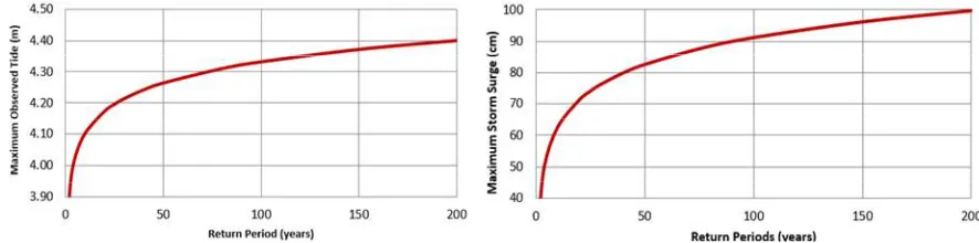
81

has demonstrated that the differences between hydrostatic and hydrodynamic models are moderate

82

at regional scale and large in a few locations for tropical cyclones, due to friction, wind and other

83

dynamic factors that affects the horizontal flood movement, however, yet small for extratropical

84

cyclones which is the case of most storms that reach the ACPM.

85

2. Materials and Methods

86

2.1. Coastal flood forcing

87

2.1.1. Sea level rise projections

88

Data from the Cascais tide gauge (TG), the oldest gauge in Portugal and in all Iberian Peninsula,

89

working since 1882, was used to estimate the first relative SLR empirical projection for the

90

Portuguese coast by [14]. The gauge is located at open coast (Figure 2), at a site of low tectonic

91

activity [15], reduced glacial isostatic adjustment (GIA) and with sea level in a considerable

92

Furthermore, [16], based on a daily average data series, concluded that the relative SLR at

94

Cascais exhibited a rate of 4.1 mm/year for the past 12 years, demonstrated the correlation between

95

Cascais TG with GMSL rates. The Cascais SLR analysis validation was performed by comparison

96

results with regional and global data models obtained from satellite and global tide gauge data, after

97

removing the difference of the corresponding vertical velocity rate effect (obtained from tectonics

98

and GIA) [5].

99

For different MSL data series and different methodological approaches, [5] show a set of

100

relative SLR projections for the 21st _{century, based on which the author generated a probabilistic}

101

ensemble used to compute a SLR probability density function at epoch 2100.

102

Based on the Cascais TG relative SLR estimation of 2.1 mm/year between 1992 and 2005 and 4.1

103

mm/year between 2006 and 2016, [5] estimated an accelerated SLR model, designated by

104

Mod.FC_2b. The central estimate of this model (Figure 1) show an intermediate hazard projection,

105

when compared with other estimations and extreme values reported by [4], with a value of 1.14 ±

106

0.15 m for epoch 2100. This Cascais TG projection model of SLR was applied to the entire ACPM to

107

produce coastal flood probabilistic maps, used consequently for coastal vulnerability and risk

108

assessment [10,11].

109

110

Figure 1. Model of relative SLR projection, Mod.FC_2b (Model 2b of FCUL), based on the analysis of

111

Cascais tide gauge data series, from 1992 to 2016 [5].

112

2.1.2. Maximum tide modelling

113

Longest tide series in Portugal are only available for the Cascais and Lagos TG, under the

114

responsibility of the national Directorate-General for the Territorial Development (DGT). For the rest

115

of the country, except for the Leixões harbor (North), the tides were only observed for short periods

116

of a few years to two decades in the tide gauges under the responsibility of the Portuguese

117

Hydrographic Institute (IH).

118

All tidal data, by convention, are referred to the vertical reference used in hydrography, the

119

chart datum (CD), defined in Portugal as the lowest low-tide (minimum low water) observed during

120

a period longer than 19 years (18.6-year Moon’s nodal period), plus an additional safety margin (a

121

foot). For all Portuguese tide ports, the CD is 2.00 m relative to the national vertical reference, the

122

1938 Cascais Vertical Datum (CASCAIS1938), except for the Tagus Estuary, where the CD is 2.08 m.

123

CD must be removed from the hydrographic tide heights to obtain the tide elevation, which

124

corresponds to the tide orthometric height relative to the national vertical reference of

125

CASCAIS1938.

126

Knowing that the maximum High Tide has a synoptic variation of 4 to 5 years (1/4 of Moon's

127

nodal period), the annual reference tide for this study corresponds to a maximum high-water level,

128

corresponding to the maximum of the equinoctial high tides. These maximum high tides occur when

129

causing the known "giant tides" or "king tides”. For this reason, the 2010 king tides chosen for this

131

national study.

132

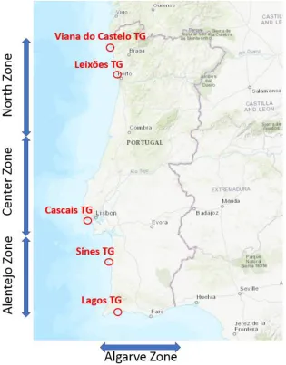
To enable a rapid and comprehensive assessment study, four tidal harbors, namely Leixões,

133

Cascais, Sines and Lagos, were chosen to estimate tides for the North, Center, Alentejo and Algarve

134

regions of the ACPM (Figure 2). This partition into four tidal zones, as it will be explained further,

135

contributed also for the terrain data model simplification, enabling the entire coastal extension

136

assessment using 20 m spatial resolution data without exceeding computing capacity demand.

137

Tide models from [17] were used to model four regional tides for the 2010reference year, from

138

which cumulative density functions (accumulated frequency or percentile function) were

139

determined (lower curve in the Figure 5, for the case of the Cascais TG).

140

141

142

Figure 2. Location of the five TG used in the study: Leixões, Cascais, Sines and Lagos for the tide

143

modeling and Viana do Castelo for storm surge analysis at the northern region.

144

2.1.3. Storm surge modelling

145

Storm Surge (SS) is the additional increase of the predicted astronomical tides caused by

146

meteorological forcing due to storm events, through the joint effect of a lower atmospheric pressure,

147

with a ratio of -1 cm/hPa, and the persistent effect of wind friction on the sea surface, depending on

148

its direction and intensity. SS is a tide level disturbance, usually positive but can also be negative

149

when high atmospheric pressure occurs, ranging from a few centimeters to several meters and that

150

can last for hours to more than a day. In Portugal, according to an update study following the

151

maximum observed storm surge, along the west coast of Portugal mainland, exhibited average

153

values ranging from 50 to 70 cm for the different TG, and maximums values of 80 cm to 1 m for long

154

return periods (100 years or more). The maximum value detected by harmonic analysis was 82 cm in

155

the Viana do Castelo TG (Figure 2) at October 15th_{, 1987, and 83 cm in the Lagos TG at March 4}th_{, 2013.}

156

In the latter, such magnitude is only explained by the additional wave setup effect due to the TG

157

localization and the SW wave direction of such storm event.

158

To evaluate and characterize the SS for the TG data series, a harmonic analysis was preformed,

159

and the maximum storm surge series were updated for further analysis through the simple Gumbel

160

distribution (Figure 3a to 3c).

161

The Viana do Castelo TG data set was used to assess the storm surge for the northern region

162

(Figure 3a), due to the absence of enough data for the Leixões TG. The Cascais TG data set was

163

applied for the central region storm surge assessment (Figure 3b), and the Lagos TG data set for

164

Alentejo and Algarve regions (Figure 3c).

165

166

Figure 3a. Return period curves for the maximum observed tide (left), relative to the TG chart datum,

167

and the maximum storm surge (right) for the Viana do Castelo TG (1978-2008 data series).

168

169

Figure 3b. Return period curves for the maximum observed tide (left), relative to the TG chart

170

datum, and the maximum storm surge (right) for the Cascais TG (1959-2018 data series).

171

172

Figure 3c. Return period curves for the maximum observed tide (left), relative to the TG chart datum,

173

and the maximum storm surge (right) for the Lagos TG (1986-2018 data series).

174

With this characterization, the maximum tide frequency, corresponding to the maximum tide

175

and extreme storm surge joint probability, the 50, 100, and 200-year return periods (RP) were

176

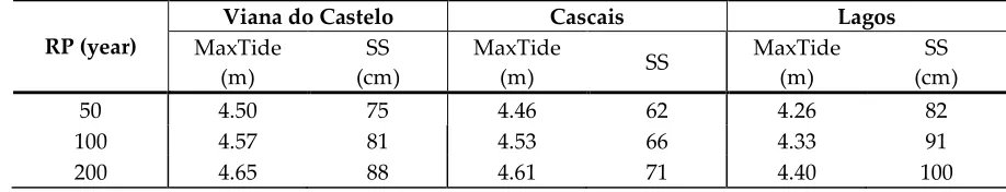
Table 1. Maximum tide height, relative to the respective TG chart datum, and storm surge (SS) for

178

the 50, 100 and 200-year return periods, for previous three TG.

179

RP (year)

Viana do Castelo Cascais Lagos

MaxTide (m)

SS (cm)

MaxTide

(m) SS

MaxTide (m)

SS (cm)

50 4.50 75 4.46 62 4.26 82

100 4.57 81 4.53 66 4.33 91

200 4.65 88 4.61 71 4.40 100

2.1.4. Wave and wind setup

180

In addition to the tide forcing and the SS, the sea level (SL) extremes are also influenced by the

181

settling effect resulting either from coastal waves in the nearshore breaking zone or from strong

182

winds, particularly in inland waters where swell waves do not reach. Thus, to estimate sea surface

183

extreme values near the coast, the wave setup must also be considered for open sea coastal areas and

184

the wind setup for the inland water areas (estuaries and coastal lagoons).

185

The model that was used for the wave setup ( ) follows the Direct Integration Method (DIM)

186

applied by [19], which includes two setup components, a static component ( ) and a dynamic

187

component :

188

(1)

The static component is given by:

189

(2)

being Hs the significant wave height (highest third of the waves, H1/3). The dynamic component is

190

defined by the combination of the setup oscillation standard deviation (σ1) and the incidence runup

191

standard deviation (σ2):

192

(3)

where

193

(4)

and

194

(5)

being m the average slope of the coast profile, the Ts the mean wave period.

195

The total effect of the wave setup coastal forcing corresponds to the overlapping of the

196

incidence runup after the wave breaking. In this study, only average estimations of wave setup

197

component, without the addition of the incidence runup effect, were considered due to the

198

impossibility of determining an accurate beach profile along Portugal mainland coastline.

199

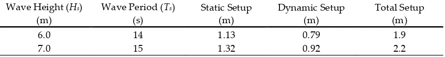
Based on the wave records time series of the Leixões and Faro wave buoys, a maximum analysis

200

was preformed using the Gumbel function. From this analysis, Hs and Ts, corresponding to RP of 10

201

and 40 years (Table 2) of 6 and 7 m, were used for the calculation of the wave setup and added to the

202

extreme tidal levels of 50 and 100 yr RP, respectively.

203

The wind setup Sv, applied only to inlets or inland waters, such as Ria de Aveiro and Ria Formosa

204

(Algarve), and Tagus Estuary, results from the following expression [20]:

205

where V10 is the wind speed at 10 m above surface and w is the sea water density. Since no references

206

were found for the region, an average wind speed of 38 km/h (10.6 m/s) was applied resulting into

207

wind setup of Sv = 0.20 m.

208

Table 2. Significant heights (Hs) and mean wave periods (Ts), corresponding to the RP of 10 and 40

209

years, respectively.

210

Wave Height (Hs)

(m)

Wave Period (Ts)

(s)

Static Setup (m)

Dynamic Setup (m)

Total Setup (m)

6.0 14 1.13 0.79 1.9

7.0 15 1.32 0.92 2.2

2.2. Methodology for Coastal Flood Scenarios

211

2.1.1. Digital Terrain Model

212

The Digital Terrain Model (DTM) used in this study was obtained from the photogrammetric

213

model provided by the DGT. The aerial photogrammetric survey for the basic cartographic data

214

acquisition along Portugal Mainland coastal strip area, of approximately 513 400 ha, was carried out

215

in 2008, with a spatial resolution of 2 m. In total, 4 139 files of elevation points (X, Y, Z), were

216

processed for the DTM calculation.

217

In order to improve the computational performance of altimetric data processing, four different

218

geographical zones were separately considered and the corresponding altimetric grid resampled at

219

20 m spatial resolution (Figure 2): North (from Viana do Castelo to Figueira da Foz), Center (from

220

Figueira da Foz to Cabo Espichel), Alentejo (from Sesimbra to Cabo de São Vicente) and Algarve (from

221

Sagres to Vila Real Santo António) (Table 1). This partition became also an advantage for the coastal

222

forcing computation, once for each zone there are different estimate scenarios with the combination

223

of Portuguese Atlantic coast SLR and the respective tide model, SS and wave setup estimations.

224

Table 3. Number of elevation points for each geographical zone.

225

Geographic Zone Extension # Elevation Points

North Viana do Castelo to Figueira da foz 3 069 154

Center Figueira da Foz to Cabo Espichel 5 845 401

Alentejo Sesimbra to Cabo de São Vicente 1 149 289

Algarve Sagres to Vila Real Santo António 1 744 278

Total 11 808 122

The positional quality control is indispensable in the production of flooding cartography due to

226

the respective impact of an incorrect risk assessment. The DTM was produced by photogrammetry

227

and, despite being a very efficient and accurate method, it is not free of errors. The respective data

228

set was generated from raw data through filtering, by classification of points in "soil" and "non soil",

229

and interpolation to fill the gaps. Errors may still occur during post-processing of the data.

230

Therefore, quality control should detect errors and deviations, however it is very difficult to link

231

certain errors (or its magnitude) to a concrete cause to be able to eliminate them [21].

232

For such purpose, the validation of the DTM was done based on a set of ground control points,

233

in a total of 134 national geodetic marks, for which the altimetric values (orthometric base height -

234

HGV) are known and hence differences from the photogrammetric DTM heights (hDTM) can be

235

estimated:

236

(7)

An overall mean square error of 56 cm was estimated with a sample of 134 control points for the

237

entire coastal area. No shift, based on the obtained residual mean, was applied to the DTM, because

238

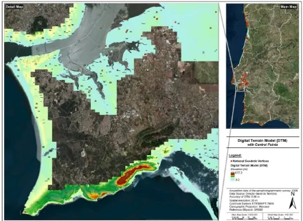
Finally, the obtained DTM (Figure 4), for the whole coastal zone of Portugal Mainland, shows values

240

between 0 m and 637.3 m with a spatial resolution of 20 m and with 56 cm of relative accuracy

241

(precision).

242

243

Figure 4. Digital Terrain Model of the Atlantic Coast of Portugal Mainland, with a spatial resolution

244

of 20 m and 56 cm of relative accuracy estimated using the National Geodetic Network.

245

2.1.2. Methodology for the probabilistic cartography

246

Based on the methodology of [22], different SLR scenarios for 2050 and 2100, with different

247

extreme events RP, and maximum tide levels were estimated based on tide historical data from the

248

Leixões, Cascais, Sines and Lagos TG. Thus, each national wide scenario is a composition of four

249

territorial zones: North, Center, Alentejo and Algarve. Except for the Cascais TG, that has the longest

250

tide series, all the other TG (Leixões, Sines and Lagos) have shorter and incomplete data series for the

251

1970 - 2010 period.

252

Considering the ACPM SLR projection (Figure 1), the tide submersion percentiles were computed

253

for the two epochs under study, 2050 and 2100. Adding the storm surge effect for two RP considered

254

(50 and 100 years), as well as wave setup, to the predicted tide level submersion frequency for each

255

reference TG, the flood levels are defined by Equations 8a and 8b.

256

(8a)

(8b)

From the resulting annual submersion percentile curves (Figure 5 shows only the case of

257

Cascais TG), the elevations for the extreme flooding levels (EFL), corresponding to the 0.25%

258

260

Figure 5. Cascais tide submersion percentile for the mean SL (blue) at epoch 2050 (left) and epoch

261

2100 (right), with storm surge (red and green) and wave setup (purple and light blue) for 50 and

262

100-year return periods.

263

To incorporate the SLR scenarios and their uncertainty into the vulnerability assessment, the

264

Extreme Flood Hazard Index (EFHI) has been defined with five probability classes ranging from 1

265

(low hazard and low probability) to 5 (extreme hazard and high probability). The EFHI is then

266

calculated by considering the uncertainty of the submersion frequency models, that result from the

267

tides standard deviation estimation, storm surge, SLR and setup. Therefore, through Equations 8a

268

and 8b, the uncertainty of extreme flood scenario is evaluated by:

269

(9a)

(9b)

270

Figure 6. Method for the flooding probability calculation and the EFHI on a generic topographic

271

profile (3.5 m, 2.5 m and 1.5 m), based on the highest tide level (h=2.5 m) and its uncertainty (adapted

272

from [22]). Intermediate EFHI levels, 2 and 4, are located between index levels 1, 3 and 5.

273

The uncertainty value of each scenario depends on the projection year, therefore the scenario

274

EFL_1 standard deviation obtained for the 2050 and 2100 epochs were 12 and 40 cm, respectively.

275

Based on the uncertainties estimated by Equation 9a, the standard normal distribution curve is

276

determined (Figure 6). This normal distribution curve has a conditional flood probability on the

277

dimension of the topographic profile, which enables the determination of the probabilistic flood level

278

projection of sea level). Subdividing the probability domain into five intervals of 20%, the EFHI is

280

defined by a five-class range, from 1 (lowest probability, from 0.25 to 20%) to 5 (maximum probability,

281

from 80 to 99.75%), related to coastal forcing (Table 4) and flooding hazard level.

282

Table 4. EFHI classification levels and respective conditional probability interval for a SLR scenario,

283

relative to the respective central flooding elevation reference level.

284

Hazard Class Level Very Low Low Moderate High Extreme

1 2 3 4 5

Flood Probability ≤ 20% 20% - 40% 40% - 60% 60% - 80% ≥ 80%

3. Results

285

The costal flood hazard cartography is produced based in the GIS tools and supported by the

286

most rigorous updated coastal DTM, referred in section §2.1.1. The flood hazard classification

287

subdivided into five classes (from 1 – Very Low Hazard to 5 – Extreme Hazard), was then used to

288

define the flooding scenarios cartography, from which the coastal physical vulnerability model is

289

further developed and evaluated [11].

290

3.1. Probabilistic cartography of coastal flood

291

The flood scenarios assessment presented here is based on a probabilistic rather than a

292

deterministic approach as explained in section §2.1.2 and is focused on the identification of areas

293

with the flooding conditional probability for the future scenarios of SLR, for the time horizon of 2050

294

and 2100.

295

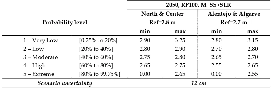
3.1.1. Year 2050

296

Table 5 shows the minimum and maximum values of each probabilistic interval corresponding

297

to the five levels of flood hazard estimated for 2050. By intersecting these elevation interval levels

298

with the DTM, the flooding areas for each scenario and geographical zone, are obtained and

299

classified into five classes of flooding hazard, represented by a given scale color in a GIS map

300

visualizer.

301

Table 5. Intervals for each EFHI level and respective probability for the 2050 SLR scenario for each

302

geographic zone, relative to the central reference flooding elevation level (Ref).

303

2050, RP100, M+SS+SLR

Probability level

North & Center Alentejo & Algarve

Ref=2.8 m Ref=2.7 m

min max min max

1 – Very Low [0.25% to 20%] 2.90 3.25 2.80 3.15

2 – Low [20% to 40%] 2.80 2.90 2.70 2.80

3 – Moderate [40% to 60%] 2.75 2.80 2.65 2.70

4 – High [60% to 80%] 2.65 2.75 2.55 2.65

5 – Extreme [80% to 99.75%] 0.00 2.65 0.00 2.55

Scenario uncertainty 12 cm

Table 6 presents the amount of area (km2_{) for each hazard class and each Portuguese coastal}

304

district for the 2050 epoch. It is possible to see that 903.2 km2 _{of Portugal coastal zone are susceptible}

305

to be flooded in an extreme scenario with 100-year RP and being Lisbon the district with the largest

306

flooding area (221.4 km2_{), followed by the Faro district (182.4 km}2_{). Although Santarém isn’t a coastal}

307

shoreline district, it is also affected by SLR scenarios due to the existence of an intertidal zone of

308

Table 6. Flooding areas (in km2_{) for each EFHI class interval and respective probability, for the 2050}

310

SLR scenario in each coastal district.

311

District 1 – Very Low [0.25% to 20%]

2 – Low [20% to 40%]

3 – Moderate [40% to 60%]

4 – High [60% to 80%]

5 – Extreme [80% to 99.75%]

Total [km2_]

Aveiro 11.8 3.2 1.7 4.0 150.7 171.4

Beja 0.2 0.1 0.0 0.1 6.3 6.6

Braga 0.7 0.2 0.1 0.2 2.6 3.7

Coimbra 4.8 0.9 0.5 1.0 33.9 41.1

Faro 8.5 3.1 1.5 2.7 166.6 182.4

Leiria 3.5 0.9 0.5 1.1 14.2 20.2

Lisbon 12.3 4.1 2.4 5.8 196.8 221.4

Porto 0.4 0.1 0.0 0.1 1.9 2.5

Santarém 12.0 4.2 2.9 4.7 75.3 99.1

Setúbal 13.7 3.6 1.9 4.0 113.6 136.8

Viana do Castelo 2.8 1.1 0.4 0.9 12.7 17.9

Total 70.7 21.5 12.0 24.5 774.4 903.2

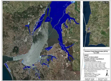
Figure 7 shows, for the ACPM, the 2050 coastal forcing scenarios probability, within a zoom of

312

the Tagus Estuary.

313

314

Figure 7. Portuguese coastal flooding extreme scenarios for 2050 SLR and 100-yr RP, within a zoom

315

of the Tagus Estuary.

316

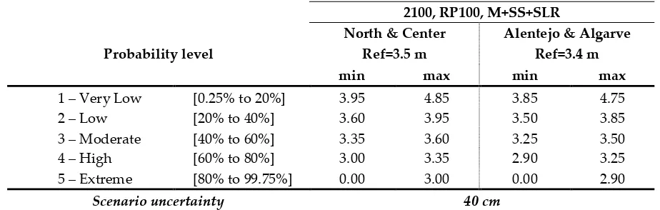
3.1.2. Year 2100

317

Table 7 shows, the minimum and maximum values of each probabilistic interval corresponding

318

Table 7. Intervals for each EFHI level and respective probability for the SLR 2100 scenario for each

320

geographic zone, relative to the central reference flooding elevation level (Ref).

321

2100, RP100, M+SS+SLR

Probability level

North & Center Alentejo & Algarve

Ref=3.5 m Ref=3.4 m

min max min max

1 – Very Low [0.25% to 20%] 3.95 4.85 3.85 4.75

2 – Low [20% to 40%] 3.60 3.95 3.50 3.85

3 – Moderate [40% to 60%] 3.35 3.60 3.25 3.50

4 – High [60% to 80%] 3.00 3.35 2.90 3.25

5 – Extreme [80% to 99.75%] 0.00 3.00 0.00 2.90

Scenario uncertainty 40 cm

Table 8 presents the sum of areas for each hazard class and each Portuguese coastal district for

322

the 2100 epoch. Besides, it is also shown that an area of 1146 km2 _{has the probability of flood in 2100,}

323

and that 74.6% of that area is classified as extreme. The Lisbon district will be again the most affected

324

with an area of 249.6 km2 _{with probability of flood.}

325

326

Figure 8. Portuguese coastal flooding extreme scenarios for 2100 SLR and 100-yr RP, within a zoom

327

of the Aveiro inland lagoon (Ria de Aveiro).

328

Table 8. Flooding areas (in km2_{) for each EFHI class interval and respective probability, for the}

329

SLR 2100 scenario in each coastal district.

330

District 1 – Very Low [0.25% to 20%]

2 – Low [20% to 40%]

3 – Moderate [40% to 60%]

4 – High [60% to 80%]

5 – Extreme [80% to 99.75%]

Aveiro 25.2 10.5 8.0 11.4 163.6 218.6

Beja 0.4 0.2 0.1 0.2 6.5 7.3

Braga 2.4 0.8 0.5 0.7 3.2 7.6

Coimbra 5.8 3.3 2.6 4.7 37.6 54.0

Faro 14.2 6.7 5.3 8.5 176.3 211.0

Leiria 7.1 3.3 2.4 3.5 17.8 34.1

Lisbon 10.5 8.2 6.6 11.2 213.2 249.6

Porto 2.0 0.6 0.4 0.4 2.2 5.7

Santarém 29.5 11.1 9.3 11.7 91.3 152.9

Setúbal 18.6 8.2 6.9 12.8 127.5 174.1

Viana do Castelo 7.1 3.1 2.1 2.9 15.9 31.1

Total 122.8 56.1 44.1 68.0 855 1146

Figure 8 shows, for ACPM, the 2100 coastal forcing scenarios probability, within a zoom of the

331

Ria de Aveiro.

332

3.2. Probabilistic cartography of extreme coastal flood with wave and wind setup

333

The extreme flood scenario with setup (EFL_2 in Equation 8b), must be separated into open sea

334

coastal areas (coastal shoreline), with the influence of ocean waves and consequently wave setup,

335

and inland water areas, only influenced by wind setup, which requires a mask to apply both

336

scenarios to the whole DTM in GIS.

337

Using the setup models values (wave setup presented in the Table 2), Table 9 shows the

338

minimum and maximum values of each probabilistic interval corresponding to the five levels of

339

flood hazard estimated for 2100. For inland water zones, a maximum wind setup of 20 cm was

340

added to the values in Table 7. The scenario uncertainty was kept the same (40 cm), due to the

341

difficulty in the estimation of the respective coupled scenario standard deviation. Knowing that the

342

most accurate uncertainty would be higher than the one adopted, the larger the flooded area would

343

be.

344

Figure 9 presents, for the Atlantic Coast of Portugal, the 2100 coastal forcing scenarios

345

probabilistic map of Ria de Aveiro. Comparing Figure 8 with Figure 9, it is possible to observe some

346

differences between them, specifically along the coastal shoreline and at the limits of the extreme

347

arms of the lagoon. In the scenario with influence of wave and wind setup, there is a larger area with

348

flooding probability, as it would be expected. This scenario is somehow realistic because storm

349

surges can sometimes be accompanied by high energetic swell waves that generates a higher storm

350

setup.

351

353

Figure 9. Portuguese coastal flooding extreme scenario with the influence of wave and wind setup, of

354

for 2100 SLR and 100-yr RP, within a zoom of Aveiro inland lagoon (Ria de Aveiro).

355

Table 9. Intervals for each EFHI level and respective probability for the SLR 2100 scenario with the

356

additional setup component for each geographic zone, relative to the central reference flooding

357

elevation level (Ref).

358

2100, RP100, M+SS+SLR+Setup

Probability level

North Center Alentejo & Algarve

Ref=7.7 m Ref=7.5 m Ref=6.9 m

min max min max min max

1 – Very Low [0.25% to 20%] 8.15 9.05 7.95 8.85 7.35 8.25

2 – Low [20% to 40%] 7.80 8.15 7.60 7.95 7.00 7.35

3 – Moderate [40% to 60%] 7.55 7.80 7.35 7.60 6.75 7.00

4 – High [60% to 80%] 7.20 7.55 7.00 7.35 6.40 6.75

5 – Extreme [80% to 99.75%] 0.00 7.20 0.00 7.00 0.00 6.40

Scenario uncertainty 40 cm

359

5. Conclusions

360

The developed methodology allows the production of probabilistic coastal flooding

361

cartography for any considered SLR projection, any coastal force model coupling and any DTM

362

spatial resolution, based on a hydrostatic model basis and considering that the respective associated

363

parameters uncertainties are provided or estimated.

364

Considering the Mod.FC_2b projection for the 2050 SLR with a SS of 50-yr RP for each TG zone,

365

a total of 903 Km2 _{of the ACPM is potentially affected by extreme flooding; being the districts of}

366

While for 2100, those values rise to 1146 Km2 _{of total area and, respectively, 250, 211 and 219 Km}2 _for

368

the same most affected districts.

369

Knowing that the DTM represents the actual coastal morphology, without any erosion effect

370

that is expected for future coastline retrieving, the present scenario for the coast shoreline with wave

371

setup is underestimated. Due to the coastal retrieving, forced by the sedimentary deficit, the increase

372

wave energy and its rotation caused by climate change, as well as, the increasing effect of SLR on

373

wave forward breaking towards inland, the flood extension and respective impact in open coast

374

shoreline areas will be certainly much greater than what is here estimated and presented.

375

As it is well known and widely studied, beach coastal areas are presently at high risk of erosion

376

due to the sedimentary deficit and slightly increase wave energy coupled with SLR, but despite their

377

economic and strategic importance, those are areas where the danger of SLR contributes less to the

378

flooding vulnerability due to the low exposure of population and infrastructure, contrary to what is

379

expected in the inland waters (river mouths, estuaries and ocean water lagoons) where the much

380

higher exposure will contribute potentially to a considerable higher risk level.

381

The probabilistic flood mapping production allows not only to quantify and qualify the flooded

382

area hazard for each scenario, but also, through the formulation and classification of the EFHI

383

combined with other physical susceptibility parameters, the future evaluation of the coastal

384

vulnerability mapping and the coastal risk assessment. These outputs are and will be fundamental

385

for coastal planning adaptation within a sustainable gradual and collaborative strategy.

386

Results contribute greatly to the identification of areas that are most vulnerable to SLR and

387

extreme events in the context of climate change, not just because it is the first SLR flood assessment

388

for the whole Portugal Mainland, but also because the coastal flooding risk is assessed and the

389

Directive 20007/60/CE objectives are implemented.

390

Funding: This research received no external funding.

391

Conflicts of Interest: The authors declare no conflict of interest.

392

References

393

1. Nerem, R.S.; Chambers, D.P.; Choe, C.; Mitchum, G.T. Estimating Mean Sea Level Change from the

394

TOPEX and Jason Altimeter Missions. Marine Geodesy 2010, Volume 33, pp.435–446. doi:

395

10.1080/01490419.2010.491031

396

2. Church, J.A.; White, N.J. Sea-Level Rise from the Late 19th to the Early 21st Century. Surveys in Geophysics

397

2011, Volume 32, pp.585–602. doi: 10.1007/s10712-011-9119-1

398

3. Hay, C.C.; Morrow, E.; Kopp, R.E.; Mitrovica, J.X. Probabilistic reanalysis of twentieth-century sea-level

399

rise. Nature 2015, Volume 517, pp.481–484. doi: 10.1038/nature14093

400

4. Sweet, W.V.; Kopp, R.E.; Weaver, C.P.; Obeysekera, J.; Horton, R.M.; Thieler, E.R.; Zervas, C. Global and

401

Regional Sea Level Rise Scenarios for the United States. NOAA Technical Report; Publisher: NOAA Silver

402

Spring, Maryland, USA, 2017, NOS CO-OPS 083.

403

5. Antunes, C. Assessment of sea level rise at west coast of Portugal Mainland and its projection for the 21st

404

century. J. Mar. Sci. Int., 7(3), 61. doi: 10.3390/jmse7030061.

405

6. Leuliette, E.W.; Scharroo, R. Integrating Jason-2 into a multiple-altimeter climate data record. Marine

406

Geology 2010, 33(sup 1), 504–517. doi: 10.1080/01490419.2010.487795.

407

7. Johnson, G.C.; Chambers, D.P. Ocean bottom pressure seasonal cycles and decadal trends from GRACE

408

Release-05: Ocean circulation implications. Journal of Geophysical Research 2013, 118(9), 228-240. doi:

409

10.1002/jgrc.20307.

410

8. Roemmich, D.; Gilson, J. The 2004–2008 mean and annual cycle of temperature, salinity, and steric height

411

in the global ocean from the Argo Program. Progress in Oceanography 2009, 82, 81–100. doi:

412

10.1016/j.pocean.2009.03.004.

413

9. McGrannahan, G.; Balk, D.; Anderson, B. The rising tide: assessing the risks of climate change and human

414

settlements in low elevation coastal zones. Environment & Urbanization 2007, 19(1), 17-37. doi:

415

10.1177/0956247807076960.

416

10. European Parliament; Council of the European Union. Floods Directive (2007/60/EC). Official Journal of the

417

European Union 2007, Vol. 50 – L288, pp. 27–34. ISSN: 1725-2555.

11. Rocha, C.S. Estudo e análise da vulnerabilidade costeira face a cenários de subida do nível do mar e

419

eventos extremos devido ao efeito das alterações climáticas. Master Thesis, Faculdade de Ciências da

420

Universidade de Lisboa, Portugal, 2016.

421

12. Costa, M.S. Desenvolvimento de uma metodologia de avaliação de risco costeiro face aos cenários de

422

alterações climáticas: aplicação ao Estuário do Tejo e à Ria de Aveiro. Master Thesis, Faculdade de

423

Ciências da Universidade de Lisboa, Portugal, 2017.

424

13. Orton, P.; Vinogradov, S.; Georgas, N.; Blumberg, A.; Lin, N.; Gornitz, V.; Little, C.; Jacob, K.; Horton, R.

425

581 New York City Panel on Climate Change 2015 report chapter 4: Dynamic coastal flood modeling. Ann.

426

N. 582 Y. Acad. Sci. 2015, 1336, 56-66.

427

14. Antunes, C.; Taborda, R. Sea Level at Cascais Tide Gauge: Data, Analysis and Results. Proceedings of the

428

10th _{International Coastal Symposium, Lisbon, Portugal, Journal of Coastal Research 2009, Special Issue 56, pp.}

429

218–222. doi: 10.2307/25737569.

430

15. Cabral, J. Neotectónica em Portugal Continental. Inst. Geol. Min. Mem. 1995, 31, 265 p.

431

16. Antunes, C. Subida do Nível Médio do Mar em Cascais, revisão da taxa actual. Proceedings of 4as

432

Jornadas de Engenharia Hidrográfica, Lisbon, Portugal, June 21-23; Instituto Hidrográfico, Eds.; 2016, pp.

433

21–24. ISBN: 978-989-705-097-8

434

17. Antunes, C. Previsão de Marés dos Portos Principais de Portugal. FCUL Webpage, 2007, Available online:

435

http://webpages.fc.ul.pt/~cmantunes/hidrografia/hidro_mares.html.

436

18. Vieira, R.; Antunes, C.; Taborda, R. Caracterização da sobreelevação meteorológica em Cascais nos

437

últimos 50 anos. Proceedings of 2as Jornadas de Engenharia Hidrográfica, Lisbon, Portugal, June 21-22;

438

Instituto Hidrográfico, Eds.; 2012, pp. 21–24. ISBN: 978-989-705-035-0

439

19. Federal Emergency Management Agency. Appendix D: Guidelines for Coastal Flooding Analysis and

440

Mapping. In Guidelines and Specifications for Flood Hazard Mapping Partners, Federal Emergency

441

Management Agency, Eds., Washington, D.C., 2002, Volume 3: Program Support, p.384.

442

www.fema.gov/fhm/dl_sgs.shtm.

443

20. Colvin, J.; Lazarus, S.; Splitt, M.; Weaver, R.; Taeb, P. Wind driven setup in east central Florida's Indian

444

River Lagoon: Forcings and pameterizations. Estuary, Coastal and Shelf Science 2018, 2013:40-48. doi:

445

10.1016/j.ecss.2018.08.004.

446

21. Höhle, J.; Höhle, M. Accuracy assessment of digital elevation models by means of robust statistical

447

methods. ISPRS Journal of Photogrammetry and Remote Sensing 2009, Volume 64, Issue 4, pp.398–406. doi:

448

10.1016/j.isprsjprs.2009.02.003

449

22. Marcy, D.; Brooks, W.; Draganov, K.; Hadley, B.; Haynes, C.; Herold, N.; McCombs, J.; Pendleton, M.;

450

Schmid, K.; Sutherland, M.; Waters K. New Mapping Tool and Techniques for Visualizing Sea Level Rise

451

and Coastal Flooding Impacts. Proceedings of the 2011 Solutions to Coastal Disasters Conference,

452

Anchorage, Alaska, United States, June 26-29; American Society of Civil Engineers, Eds.; 2011, pp.

453

474–490. doi: 10.1061/41185(417)42

454