On the implicit density based OpenFOAM solver for turbulent compressible flows

(1)

On the implicit density based OpenFOAM solver for turbulent

compressible ﬂows

Jiˇr´ı F¨ursta

Czech Technical University in Prague, Karlovo n´am. 13, 121 35 Praha 2, Czech Republic

Abstract. The contribution deals with the development of coupled implicit density based solver for com-pressible flows in the framework of open source package OpenFOAM. However the standard distribution of OpenFOAM contains several ready-made segregated solvers for compressible flows, the performance of those solvers is rather week in the case of transonic flows. Therefore we extend the work of Shen [15] and we develop an implicit semi-coupled solver. The main flow field variables are updated using lower-upper sym-metric Gauss-Seidel method (LU-SGS) whereas the turbulence model variables are updated using implicit Euler method.

1 Introduction

The OpenFOAM package [20] is widely used open source toolbox for computational fluid dynamics (CFD). The keystone of the package is a library written in object oriented C++ alowing simple manipulation with fields related to cells, vertices, or nodes of three-dimensional polyhedral meshes. The toolbox contains also several ready-made solvers for incompressible as well as compressible flows based on the finite volume method. The Open-FOAM originated from the so-called pressure based seg-regated velocity-pressure correction methods devised orig-inally for the incompressible Navier-Stokes equations, see eg. SIMPLE [4] or PISO [7]. However these segregated methods have been later extended to compressible flow problems including transonic or supersonic flows [12], the efficiency of the segregated methods is in the case of high speed flows usually worse when comparing with the so-called density based or coupled methods available in some commercial packages and in some academic in-house codes.

So far several attempts have been done in order to de-velop density based solvers for OpenFOAM. First of all, there is already a solver based on central-upwind scheme of Kurganov and Tadmor [6] in the standard distribu-tion. Next, the OpenFOAM-extend version of the pack-age contains some coupled solvers based on AUSM+up [9], HLLC [17], Roe or Rusanov fluxes combined with an explicit Runge-Kutta method in time. Similar capa-bilities has also the AeroFOAM package developed at the Politecnico di Milano. The main deficiency of the above mentioned solvers is the explicit time integration which puts a severe stability bound on the maximum time step and the efficiency of these explicit methods is much lower than the efficiency of implicit methods. This

a _{Corresponding author: [email protected]}

is especially true for high speed flows at high Reynolds number where the correct resolution of thin boundary layer requires very fine meshes. Let’s note also the hy-brid pressure-density based method [21], which is based on the AUSM+up fluxes, but still uses a pressure cor-rection loop similar to PISO algorithm and the maximal time step is therefore also limited.

The fully implicit coupled methods (see eg. [5], [3]) provides much better efficiency usually at the price of much higher complexity of the code and higher mem-ory requirements. Besides the fully implicit method the matrix-free LU-SGS (lower-upper symmetric Gauss-Seidel, [3]) method shares the appealing properties of fully im-plicit methods (i.e. the unconditional stability) with low code complexity and low memory overhead. In their re-cent paper [15] Shen at al. give detailed description of the implementation of LU-SGS method in the frame-work of OpenFOAM for the case of inviscid compressible flows. We follow their work and extend the LU-SGS based solver to turbulent flows described by the set of Reynolds-averaged Navier–Stokes equations combined with an ad-ditional turbulence model provided by the OpenFOAM package.

2 Mathematical model

2.1 Governing equations

The governing equations expressing the conservation of mass, momentum, and energy are given as follows

∂ρ

∂t +∇(ρU) = 0, (1)

∂(ρU)

∂t +∇(ρU⊗U) +∇p=∇τ, (2) ∂(ρE)

(2)

where ρis the density,U is the velocity vector, pis the pressure,τ is the (effective) stress tensor,Eis the specific total energy,λis the (effective) thermal conductivity, and T is the temperature. The system is closed by the equa-tion of state for ideal gasp/ρ=rT and constant specific heat capacitycp.

Spatial derivatives at the left hand side of the previous equations represent inviscid terms whereas the right hand side represents viscous terms. The above equations can be expressed in the integral form suitable for ﬁnite volume approximation as follows (assuming ﬁxed control volume Ω)

d dt

ΩW dΩ +

∂Ω

(Fc−Fv)dS= 0, (4)

whereW = [ρ, ρU, ρE] is the vector of conservative vari-ables andF andFvrepresent inviscid and viscous fluxes. In the case of turbulent flow the above mentioned sys-tem of equations is coupled to an additional turbulence model (e.g. a two-equation SST model [10]) which pro-vides components of the Reynolds stress tensor and the turbulent heat flux.

2.2 Spatial discretization

The numerical solution is obtained with the finite vol-ume method in semi-coupled fashion. It means that the code updates in each step the main flow variables W and then it updates the turbulence model variables. Since we are using turbulence models provided by the Open-FOAM package, we do not give detailed description of its discretization and we focus the attention to the dis-cretization of the equations for main flow variables (4).

The integral form of the equations (4) discretized in space using collocated ﬁnite volume method (FVM) by taking

Wi(t) =_|1 Ωi|

Ωi

W(x, t)dΩ, (5)

where Ωi is the mesh celli. Hence the equation (4) can be approximated as

|Ωi|dWi

dt =−R(W)i=−

j∈Ni

(Fij+Fijv), (6)

where Ni is the set of indices of neighbor cells and Fij and F_ijv are the numerical fluxes approximating the in-viscid and viscous fluxes. Viscous fluxes are discretized directly with OpenFOAM built-in schemes (e.g. central scheme). On the other hand the discretization of inviscid fluxes is made using well established approximate Rie-mann solvers. The first order Rusanov convective flux is

FRus

ij = F(Wi) +₂ F(Wj)·Sij−λ₂ij (Wi−Wj), (7)

where the inviscid ﬂux matrixF is

F(W) = ⎡

⎣_ρU_⊗ρU_U+pI (ρE+p)U

⎤

⎦_, (8)

and the stabilization parameterλij is

λij =|Uij·Sij|+|Sij|aij. (9)

HereU_ij is the velocity at the face shared by cell iand j (it can be taken as an arithmetic average of U_i and Uj) andaij is the sound speed at the face. The Rusanov ﬂux together with the viscous terms forms a low order rezidual

Rlo₍_W₎ i=

j∈Ni

FRus₍_WL

ij,WijR,Sij) +Fijv

. (10)

The residual can be further simpliﬁed using the fact that

jSij= 0, so

Rlo₍_W₎ i =1₂

j∈Ni

(F(W_j)·S_ij+λijWj)−

−1 2

⎛

⎝

j∈Ni

λij ⎞

⎠_W_i+

j∈Ni

Fv ij. (11)

It is well known that the Rusanov flux is overly dif-fusive and it is not a good choice for high speed flows. On the other hand thanks to its simplicity one can eas-ily calculate the Jacobian matrix∂R/∂W, see next sec-tions. In order to improve the accuracy a better Riemann solver should be used in the evaluation of the residual. In our the AUSM+up flux [9] or HLLC [17] flux is em-ployed together with a piece-wise linear reconstructions with Barth [2] or Venkatakrishnan [18], thus the high or-der rezidual is

Rho_(W₎ i=

j∈Ni

Fho_(WL

ij,WijR,Sij) +Fijv

. (12)

HereFhois the AUSM+up or HLLC ﬂux evaluated from the reconstructed states at the left (WL_{) and right (W}R₎ hand side of the face.

2.3 Temporal discretization

The temporal discretization is achieved by using the im-plicit Euler method, thus

Wn+1

i =Win−_|Δt_Ω_i|Rho(Wn+1)i. (13)

The large system of non-linear equations is then linearized

Wn+1

i ≈Win−_|Δt_Ω i|

⎛

⎝_Rho₍_Wn₎ i+

j∈Ni∪{i}

∂Rho i ∂WjΔWj

⎞

⎠_,

(14) withΔW =Wn+1−Wn, thus

j∈Ni∪{i}

_| Ωi| Δtδij+

∂Rho i ∂Wj

ΔWj=−Rho(Wn)i. (15)

DOI: 10.1051/

, 02027 (2017) 714302027

143

EPJ Web of Conferences epjconf/201

(3)

Finally the Jacobian matrix of high order residual at the left hand side is replaced by its low order approximation, so

j∈Ni∪{i}

|Ωi|

Δtδij+ ∂Rlo

i ∂Wj

ΔWj=−Rho(Wn)i. (16)

The matrix of the linear system (16) can be divided into block diagonal partD, the lower triangular matrixL and the upper triangular matrix. Replacing the Jacobian matrices of viscous ﬂuxes by their spectral radii [3] and assuming local time step one ﬁnally arrives to diagonal operatorD in the form

Di= ⎛

⎝Ωi

Δti + 1 2

j∈Ni

λ∗_ij ⎞

⎠_I. (17)

The spectral radiusλ∗_ij is composed of the inviscid con-tribution λij given by (9), an over-relaxation parameter ωin the range 1≤ω≤2, and the viscous spectral radius λv_ij [3]

λv_ij = |Sij|

||xi−xj||max

4 3ρij,

γ ρij

μ P r +

μT P rT

, (18)

thus

λ∗_ij=ωλij+λvij. (19) Let us deﬁne the sets of cells belonging to lower and upper part of the matrix:

Li={j∈Ni:j < i}, (20) Ui={j∈Ni:j > i}. (21)

Then the matrix-free LU-SGS scheme can be written using the following two step procedure:

DiΔWi(1)=−Rhoi −1₂

j∈Li

ΔF_j(1)·Sij+λ∗ijΔWj(1)

,

DiΔWi=DiΔWi(1)− 1 2

j∈Ui

ΔFj·Sij+λ∗ijΔWj.

Here

ΔW_i(1) =W_i(1)−W_in, (22) ΔF_i(1) =F(W_i(1))−F(W_in), (23) ΔFi =F(Win+1)−F(Win). (24)

2.4 Coupling with a turbulence model

The LU-SGS solver is combined with an additional tur-bulence model in a weakly-coupled manner. It means that the turbulence quantities (e.g.kandωin the case of two-equation SST model) are kept ﬁxed during one iteration of LU-SGS model. Then these variables are updated us-ing appropriate model keepus-ing the vector of conservative variable constant. Hence (for the case of SST model:

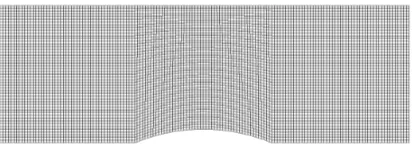
Fig. 1.Structured mesh for the ﬂow over a bump.

1. calculate Wn+1 from Wn using both steps of LU-SGS method (22) and assuming ﬁxedkn andωn, 2. calculatekn+1 andωn+1 using ﬁxedWn+1.

The advantage of the semi-coupled approach is that it allows inclusion of built-in OpenFOAM turbulence mod-els. Moreover, the implementation is much simpler than it would be in the fully-coupled scheme.

3 Results

3.1 Subsonic ﬂow over a bump

The two-dimensional subsonic flow over a 10% circular bump has been chosen as a first benchmark. The invis-cid flow passes through a channel of height H = 1 m and length L = 3 m. The total pressure at the inlet was ptot,in = 100 kPa, the total temperature Ttot,in = 293.15 K and the inlet flow direction was parallel to x -axis. The average outlet pressure corresponds to isen-tropic Mach numberMis,out= 0.1. The solution was ob-tained using a structured mesh with 150×50 quadrilat-eral cells, see fig. 1.

(4)

Fig. 2. Mach number distribution for subsonic ﬂow over a bump.

Fig. 3.Mach number distributen over the lower wall for sub-sonic ﬂows over a bump.

Fig. 4. Convergence history for subsonic ﬂows over a bump.

Fig. 5. Mach number distribution for transonic ﬂow over a bump.

3.2 Transonic ﬂow over a bump

The second benchmark is a transonic ﬂow over the bump using the same geometry as in the previous case. The same boundary conditions were used at the inlet and the average outlet pressure was set to a value corresponding to isentropic Mach numberMis,out = 0.675. In this case the ﬂow accelerates over the bump and reaches supersonic speed. Then it passes through a shock wave and continues towards the outlet.

The figure 5 shows the contours of Mach number ob-tained with LU-SGS scheme with AUSM+up flux and piecewise linear reconstruction with Venkatakrishnan lim-iter. The sonic line (i.e. the line where the magnitude of the velocity equals to local sound speed is plotted in other color in order to depict the shape of the supersonic region. The comparison of the Mach number over the lower wall is shown in the figure 6. One can see that all methods including the transonic variant of SIMPLE solver give similar results. Nevertheless the resolution of the shock wave is much better with the AUSM or HLLC based LU-SGS scheme than with the SIMPLE solver which spreads the shock over 4 cell due to higher amount of numerical viscosity. The figure 7 compares the convergence history for all solvers. One can see that the LU-SGS scheme is more efficient than the segregated approach in this case. Note that the CPU time for 10000 iterations was approx-imately the same using all methods including segregated SIMPLE solver.

3.3 Transonic ﬂow through a turbine cascade

The next benchmark is two-dimensional compressible tur-bulent ﬂow through test turbine cascade SE-1050. The geometry and boundary conditions correspond to the test from ERCOFTAC QNET database [13]. The inlet total presuure and total temperature were ptot,in = 100 kPa and Ttot,in = 293.15 K and the inlet angle was αin = 19.3◦. The average outlet pressure corresponds to isen-tropic outlet Mach numberMis,out = 1.2, the Reynolds number related to outlet ﬂow conditions and blade pitch was Re = 1.2×106 and the inlet turbulence intensity wasT uin= 2 %.

DOI: 10.1051/

, 02027 (2017) 714302027

143

(5)

Fig. 6.Mach number distributen over the lower wall for tran-sonic ﬂows over a bump.

Fig. 7.Convergence history for transonic ﬂows over a bump.

The hybrid mesh was composed of structured quadri-lateral layer around the blade and unstructured triangu-lar part in the rest of the domain. The mesh contained ap-proximately 66×103 cells and the near-wall refinement corresponded to y+₁ ≈ 0.2. Details of the mesh around leading and trailing edges is given at the figure 8. The figure 8 shows contours of the Mach number in two pe-riods of the mesh obtained using LU-SGS scheme with HLLC flux. One can see here both branches of the shock emanating from the trailing edge as well as the interac-tion of the inner branch of the shock wave with the blade. The figure 10 shows the comparison of the pressure along the blade with the results obtained with segregated SIM-PLE solver as well as with the experimental data [13]. One can see that both numerical methods shows very good agreement with experimental data.

(a) Leading edge (b) Trailing edge

Fig. 8.Hybrid mesh for test turbine cascade.

Fig. 9.Calculated Mach number distribution in the test tur-bine cascade.

3.4 Transonic ﬂow through 3D test turbine cascade

(6)

Fig. 10. Pressure distribution over the test turbine blade, comparison with experimental data [13].

Fig. 11. Pressure distribution at the blades and side wall and the entropy distribution in test plane for the 3D ﬂows over test turbine cascade.

in the vicinity of side walls. The figure 12 shows the com-parison of the spanwise distribution loss coefficientζ(see [16]) obtained using LU-SGS scheme with HLLC flux and the transonic version of segregated SIMPLE solver with experimental data. One can see that the loss coefficient is better predicted by LU-SGS method especially in the middle of the channel.

3.5 Transitional ﬂow through VKI turbine cascade

The last case demostrates the combination of the LU-SGS scheme for main flow variables with transitional tur-bulence models. The test case corresponds to the experi-mental study of Arts et al. [1] performed at the von Kar-man Institute for Fluid Dynamics. The 2D flow through a turbine cascade was measured in terms of surface heat flux. The numerical solution was obtained with 62 000

Fig. 12. Spanwise distribution of pitch averaged loss coeﬃ-cientζ, comparison with experiment.

Fig. 13.Surface heat transfer coeﬃcient for VKI MUR 241 Cascade.

cells for the regime corresponding to MUR 241 case from [1], i.e. the outlet Mach number was M2 = 1.089, the Reynolds number related to outlet parameter and chord length was Re = 2.1×106 and the free-stream turbu-lence intensity wasT u = 6 %. The figure 13 shows the comparison of experimental data with numerical results obtained with a three-equationk−kL−ω model devel-oped by Walters and Cokljat, see [19] or [8], and with a three-equationγ−SST model by Menter et al. [11]. One can see that both models capture very well the heat flux in the laminar part of the flow, the transition onset at the suction side is better predicted by the γ−SST model, and the heat flux is over-predicted by both models in the rear part of the suction side.

4 Conclusion

The matrix-free steady-state LU-SGS solver for compress-ible turbulent ﬂow is described. The solvers shows very

DOI: 10.1051/

, 02027 (2017 ) 714302027

143

(7)

good accuracy for several test cases ranging from inviscid low Mach number flow over a bump to transonic turbu-lent flow through turbine cascade. The convergence to steady state is superior to segregated SIMPLE solver in the case of transonic flows. The convergence is a bit worse for low Mach number flows but it should be possible to improve it using a preconditioning. The LU-SGS solver provides very robust method which doesn’t need any case dependent tuning (like e.g. relaxation factors in SIM-PLE method for transonic flows). The main advantage of OpenFOAM platform is that the LU-SGS solver can be combined with a lot of built-in turbulence models as well as with the post-processing or parallel computing provided by the platform.

Acknowledgements. This research has been realized using the support of the Czech Science Foundation under grant P101/12/1271.

References

[1] ARTS, T., LAMBERT DE ROUVROIT, M., and RUTHERFORD, A.W.Aero-thermal investigation of a highly loaded transonic linear turbine guide vane cascade: A test case for inviscid and viscous ﬂow computations. Technical Note 174. Von Kar-man Institute for Fluid Dynamics, 1990, p. 97. [2] BARTH, Timothy and JESPERSEN, Dennis. “The

design and application of upwind schemes on un-structured meshes”. In: 27th Aerospace Sciences Meeting. Reston, Virigina: American Institute of Aeronautics and Astronautics, 1989.

[3] BLAZEK, Jiri.Computational ﬂuid dynamics : prin-ciples and applications. Butterworth-Heinemann, 2015, p. 466.

[4] FERZIGER, Joel H. and PERIC, Milovan. Com-putational Methods for Fluid Dynamics. Springer Science & Business Media, 2012, p. 426.

[5] F ¨URST, Jiˇr´ı. “A weighted least square scheme for compressible ﬂows”. In:Flow, Turbulence and Com-bustion 76.4 (2006), pp. 331–342.

[6] GREENSHIELDS, Christopher J. et al. “Imple-mentation of semi-discrete, non-staggered central schemes in a colocated, polyhedral, ﬁnite volume framework, for high-speed viscous ﬂows”. In: Inter-national Journal for Numerical Methods in Fluids 63.1 (2010), pp. 1–21.

[7] ISSA, R.I. “Solution of the implicitly discretised ﬂuid ﬂow equations by operator-splitting”. In: Jour-nal of ComputatioJour-nal Physics 62.1 (1986), pp. 40– 65.

[8] KOˇZ´IˇSEK, Martin et al. “Implementation of k-kL-ω Turbulence Model for Compressible Flow into OpenFOAM”. In: Applied Mechanics and Materi-als 821 (2016), pp. 63–69.

[9] LIOU, Meng-Sing. “A sequel to AUSM, Part II: AUSM+-up for all speeds”. In:Journal of Compu-tational Physics 214.1 (2006), pp. 137–170.

[10] MENTER, F. R. “Two-equation eddy-viscosity tur-bulence models for engineering applications”. en. In:AIAA Journal 32.8 (1994), pp. 1598–1605. [11] MENTER, Florian R. et al. “A one-equation local

correlation-based transition model”. In:Flow, Tur-bulence and Combustion95.4 (2015), pp. 583–619. [12] MOUKALLED, F. and DARWISH, M. “A High-Resolution Pressure-Based Algorithm for Fluid Flow at All Speeds”. In:Journal of Computational Physics 168.1 (2001), pp. 101–130.

[13] ˇSAFA ˇR´IK, Pavel. “Experimental data from opti-cal measurement tests on a transonic turbine blade cascade”. In:13th Symposium on Measuring Tech-niques for Transonic and Supersonic Flow in Cas-cades and Turbomachines. Ed. by G. Gyarmathy) C. GROSSWEILER. ETH Zurich, 1996, pp. 0–14. [14] SHEN, Chun, SUN, Fengxian, and XIA, Xinlin.

“Implementation of density-based solver for all speeds in the framework of OpenFOAM”. In: Computer Physics Communications 185.10 (2014), pp. 2730– 2741.

[15] SHEN, Chun et al. “Implementation of density-based implicit LU-SGS solver in the framework of OpenFOAM”. In: Advances in Engineering Soft-ware 91 (2016), pp. 80–88.

[16] ˇSIMURDA, David, F ¨URST, Jiˇr´ı, and LUXA, Mar-tin. “3D ﬂow past transonic turbine cascade SE 1050 - Experiment and numerical simulations”. In: Journal of Thermal Science 22.4 (2013), pp. 311– 319.

[17] TORO, Eleuterio F. “The HLL and HLLC Rie-mann Solvers”. In:Riemann Solvers and Numerical Methods for Fluid Dynamics. Berlin, Heidelberg: Springer Berlin Heidelberg, 1997, pp. 293–311. [18] VENKATAKRISHNAN, V. “On the accuracy of

limiters and convergence to steady state solutions”. In:31st Aerospace Sciences Meeting & Exhibit(1993), pp. 1–10.

[19] WALTERS, D. Keith and COKLJAT, Davor. “A three-equation eddy-viscosity model for Reynolds-averaged Navier–Stokes simulations of transitional ﬂow”. In:Journal of Fluids Engineering130.12 (2008), pp. 121401–121401–14.

[20] WELLER, H. G. et al. “A tensorial approach to computational continuum mechanics using object-oriented techniques”. In:Computers in Physics12.6 (1998), p. 620.