High Speed FPGA Model Implementation
for Ferroelectric and Ferromagnetic Transducers
Operating in Hysteretic Regimes
Thomas R. Braun
∗and Ralph C. Smith
†Center for Research in Scientific Computation
Department of Mathematics
North Carolina State University, Raleigh, NC 27695
ABSTRACT
Ferroelectric and ferromagnetic materials are employed as both actuators and sensors in a wide variety of applications including fluid pumps, nanopo-sitioning stages, sonar transducers, vibration control, ultrasonic sources, and high-speed milling. They are attractive because the resulting transducers are solid-state and often very compact. However, the coupling of field to mechanical deformation, which makes these materials effective transducers, also introduces hysteresis and time-dependent behavior that must be accommodated in device designs and models before the full potential of compounds can be realized. Whereas a model-based control can account for these effects, the computational complexity of the model often renders this approach prohibitive. In this pa-per, we discuss a field programmable gate array (FPGA) implementations of the homogenized energy model for ferroelectric and ferromagnetic materials, and show that this approaches can yield up to over two orders of magnitude improvement in computation time when compared to a Pentium IV processor. Model formulations both including and neglecting thermally activated effects are considered.
1. Introduction
1.1. Ferroelectric and Ferromagnetic Materials
Ferroelectric and ferromagnetic materials are increasingly considered as ac-tuators and sensors for aerospace, aeronautic, and industrial automotive appli-cations due to their unique transduction capabilities. Actuator capabilities are derived from the converse effect in which input fields produce deformations in the material whereas the direct effect, comprised of stress-induced fields, pro-vides the materials with sensor capabilities. Ferroelectric materials are presently employed in microphones, accelerometers, fluid pumps, nanopositioning stages, sonar transducers, vibration sensors and actuators, ultrasonic sources, inkjet printers, and camera focusing mechanisms. Ferromagnetic transducers are typ-ically bulkier than their ferroelectric counterparts, due to the circuitry and housing required to produce magnetic fields, but they generally provide greater input forces. They are also presently being considered for a wide variety of ap-plications including torque sensors, high-speed milling, ultrasonic sources, sonar transduction, and vibration sensing and attenuation. Details regarding present and predicted applications can be found in [17].
However, the electromechanical and magnetomechanical coupling mecha-nisms that endow the compounds with unique transducer capabilities also pro-duce hysteresis and constitutive nonlinearities that must be accommodated in designs before the multifunctional material attributes can be fully realized. For certain applications, these nonlinear effects can be minimized by restricting input field levels; however, this limits the applicability of the materials. For fer-roelectric devices, hysteresis can often be mitigated through the use of charge or current controlled amplifiers [8, 9, 10, 11]. However, this is often significantly more expensive then using voltage controlled amplifiers and current control is ineffective if maintaining a DC bias as required for many positioning mech-anisms. A third alternative is to linearize hysteretic devices using feedback control. Whereas effective at lower frequencies, this technique becomes less ef-fective at higher frequencies if sampling rates are limited. Moreover, extensive linearization can limit control authority for prescribed tasks such as vibration attenuation or reference signal tracking.
To fully utilize the unique transduction capabilities of ferroelectric and fer-romagnetic materials for high performance applications, it is thus necessary to construct models that are appropriate for material characterization, device de-signs, and control implementations. These objectives dictate that the models quantify hysteresis and constitutive nonlinearities in a manner that is sufficiently accurate to meet design specifications and sufficiently efficient to permit real-time implementation. Moreover, models must be efficiently inverted to provide filters which approximately linearize transducer dynamics for subsequent linear control design.
basis, which permits correlation of parameters with measured properties of data, and its capability to characterize a wide range of physical behaviors including closer of biased minor loops in quasistatic regimes, thermal relaxation or creep, reversible behavior prior to switching, and temperature-dependent dynamics — see [17] for a comparison and contrast between the modeling frameworks.
We note that FPGA implementation for the forward and inverse Preisach model is reported in [25]. The model framework considered here differs quite substantially in that it incorporates rate, stress, and temperature-dependencies that are inherent to the materials in many operating regimes but are not incor-porated in the classical Preisach framework.
In [2], we developed a highly efficient formulation for the homogenized en-ergy model. Herein, we will employ that formulation to implement the model in field programable gate-arrays (FPGAs), and show that this yields a signif-icant decrease in computation time while maintaining sufficient accuracy. In Section 2, we briefly introduces the homogenized energy model. Following this, the FPGA implementation of the model with negligible thermal relaxation is discussed in Section 3, and results are given comparing the FPGA implementa-tion to floating point C code. In Secimplementa-tion 4, we discuss and gives results for the model formulation that includes thermal relaxation. First, however, we briefly review FPGA architecture and our particular development method for those not familiar with the technology.
1.2. Field Programmable Gate Arrays (FPGAs)
As the name suggests, an FPGA is a user-configurable hardware chip. At the physical level, it is composed of a large grid of lookup tables, flip-flops, and programmable interconnects. Many FPGAs also offer memory blocks, multipli-ers, and other similar constructs embedded in the silicon. The look-up tables can be programmed to implement the functionality of nearly any basic gate, and interconnected to implement arbitrary functions. This flexibility is what gives the FPGA the ability to operate much faster than a standard processor such as you might find in your personal computer, but also significantly increases the complexity in programming the device.
FPGAs, we must therefore speak of two different numbers when referring to the computation time of an algorithm. The throughput is the number of inputs the algorithm can handle in a given period of time and is a function of the pipelining in the chip. For the homogenized energy model, we will refer to throughput as the number of timesteps per second the FPGA is capable of processing. The other number is latency; i.e., the delay from when an input enters the FPGA or algorithm and when it exits it. The latency in our example is two clock cycles, while the throughput is the same as the FPGA clock frequency.
This is example is somewhat fabricated, as processors typically are run at a much higher clock frequencies than FPGAs are capable of running. Thus, in this example the processor would be the better choice. However, if the summation was over 1000 values instead of four, the FPGA could maintain a throughput equal to its clock frequency, while the latency would increase to ten clock pe-riods. The processor would need 999 clock ticks for each input vector, and the FPGA is likely to be faster. The speed increase in the FPGA therefore depends on how well the model can be parallelized and pipelined. The more that these two operations can be performed, the better the speed advantage will be over a desktop processor or embedded microprocessor.
The flexibility afforded by FPGAs for parallelization and pipelining does come at the cost of increased programming complexity. Vendor or third-party tools alleviate the user from determining the individual placement and routing of resources on the chip. Nonetheless, the programming process is more detailed for an FPGA. For a processor, only the operations you wish to perform and the order to perform them in need be specified in the code. Further, since the adders, multipliers, etc. are already present in the silicon, many processors allow floating point operations for little to no additional cost in computation time. With the FPGA, parallelization and pipelining/delay must be explicitly given, and numbers are not restricted to a fixed size. If only 7 bits are needed to store a given value, the FPGA allows you to allocate only 7 bits. This saves FPGA resources over using a 16 or 32 bit number, which in turn allows more parallelization. However, the size of every value between every operation must also be set when programming the device. Floating point operations are possible as well; however these typically require more FPGA resources than their fixed point (integer) arithmetic counterparts and thus are often avoided.
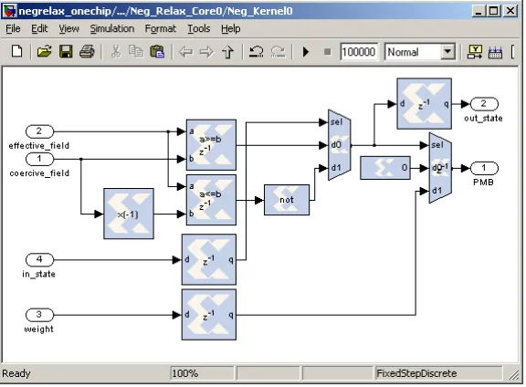
one of the leading FPGA manufacturers. This tool is an add-in for Simulink, the graphical programming engine that comes with MATLAB, and provides an additional set of blocks that can be included and connected in Simulink models. Design is performed and tested in Simulink and then converted to VHDL or Verilog at the click of a button. A screenshot depicting some of these blocks may be observed in Figure 1. The tool is moderately low-level; it will assume some defaults for bit widths, but in most cases bit widths, parallelization, and pipelining/delay must be explicitly set. However, the ability to test the design in Simulink aids in debugging and the learning curve for the tool is not as steep as VHDL or Verilog. In the authors’ opinion, modifications to a design can also be achieved more quickly with System Generator than with a hardware description language, even if the initial design time is about the same for both. Moreover, since the tool connects preexisting and highly optimized HDL code together to produce the design, System Generator derived designs tend to be as efficient as designs hand-coded in VHDL or Verilog.
If there is variety of choice when it comes to programmming tools, there is greater variety when it comes to choosing the FPGA itself. Several different manufacturers exist, all of whom offer slightly different architectures. Our choice to use System Generator dictated the use of Xilinx FPGAs. However, there are numerous sizes of FPGAs, with the classic trade-of of FPGA resources and price. There are also numerous vendors of boards which incorporate FPGAs. We chose a prototyping system from Lyrtech Signal Processing that provides all the necessary framework and board models for System Generator, allowing
code to be compiled directly from Simulink to the FPGA without the need to manipulate or interconnect anything in VHDL or Verilog. This board contains two Xilinx Virtex II 3000 FPGAs as well as four Texas Instruments floating point digital signal processors. However, for the purposes of this paper, we will consider only a single Virtex II 3000 chip. This is a relatively small chip by today’s standards, and thus is relatively affordable. Prices can very widely, but Xilinx recently released an evaluation board (DO-DI-DSP-DK4) for $2500 containing a Virtex IV SX35 chip, which is similar in size to the Virtex II 3000, along with a 14 bit analog to digital converter operating at 105 Mega-samples per second. The Virtex II 3000 (speed grade 4) part employed for the results in this paper, not counting any boards or software utilities, can be obtained online for around $800 (prices as of September 2007). Much larger chips are currently on the market, and we will allude to the advantages a larger size chip would yield at the end of this paper; however, the results presented here are designed to fit a price-point that should be easily obtainable for most high-precision applications.
2. Homogenized Energy Model
We summarize here the homogenized energy model for ferroelectric and fer-romagnetic materials [4, 2, 17, 18, 19, 22, 23] under the assumption of a constant applied load (extensions for varying loads may be found in [1, 3]). To simplify the discussion, we develop it in the context of ferroelectric materials and note that analogous relations hold for ferromagnetic compounds. We note that this is a multiscale approach in which mesoscopic (domain) behavior is quantified via energy principles and a macroscopic model is subsequently constructed via stochastic homogenization techniques. The macroscopic ferroelectric model is
P(E;x+) =
Z ∞
0
Z ∞
−∞
νc(Ec)νI(EI)[P(E+EI;Ec;x+)]dEIdEc (1)
whereP denotes the polarization,Eis the electric field,Ecdenotes the coercive field value at which the dipoles change orientation,EI quantifies the interaction field due to dipole interactions,x+ is an internal material state (defined later),
andP is a mesoscale polarization relation. The two model parametersEc and
EI are assumed to vary throughout the material according to the densities νc and νI. As detailed in [17], the densities are constrained by the the physical relations:
1. bothνc andνI are bounded by decaying exponentials, 2. νc is strictly positive,
3. νI is symmetric about 0, and 4. R∞
0 νc(Ec)dEc= 1,
R∞
−∞νI(EI)dEI = 1.
(2)
The integrals in (1) are solved numerically via quadrature relations; that is,
P(E;x+) =
Nc
X
i=1
NI
X
j=1
wherewc andwI give the quadrature weights.
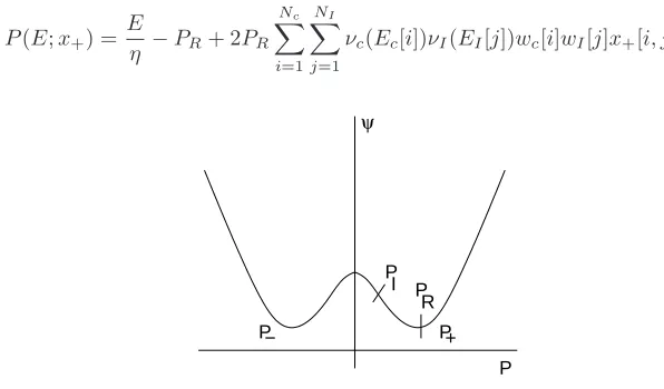
The kernelP is modeled via energy principles. The mesoscopic Helmholtz energy is taken to be
ψ(P) =
η(P+PR)2/2, P≤ −PI
η
2(PI −PR)
P2
PI
−PR
, |P|< PI
η(P−PR)2/2, P≥P
I
(4)
wherePI =PR−Ec/ηdenotes the positive inflection point at which the dipoles switch orientation,PRis the local remanence polarization, andηis the reciprocal slope ∂E
∂P. This energy relation is plotted in Figure 2. The Gibbs free energy
G=ψ−EP (5)
balances this internal Helmholtz energy with the electrostatic energy; i.e., work performed by the applied external field. As detailed in [17], where the Legendre transform properties of the Gibbs energy are discussed, Gis a function of the independent variableE and the dependent variableP.
2.1. Negligible Relaxation Model
For regimes in which thermal relaxation is negligible, direct minimization of (5) yields the kernel
P(E+EI, x+) = E+EI
η + 2PRx+−PR (6)
wherex+= 1 for positively oriented dipoles andx+= 0 for negatively oriented
dipoles. For algorithm development,x+ is set to 1 wheneverE+EI > Ec and is set to 0 wheneverE+EI <−Ec. Substituting (6) into (3) and simplifying yields
P(E;x+) = E
η −PR+ 2PR
Nc
X
i=1
NI
X
j=1
νc(Ec[i])νI(EI[j])wc[i]wI[j]x+[i, j]. (7)
P
ψ
+ P P−
P I
R P
Note that the quadrature weights and density heights can multiplieda-priori, and that x+ is either 1 or 0. Thus, the negligible relaxation model can be
implemented with NcNI + 1 additions and 2NcNI conditional statements per timestep. It should be noted that although the motivation is different, the negligible relaxation homogenized energy model is analogous to the Preisach model for ferroelectric or ferromagnetic materials if the limit is taken asη→ ∞.
2.2. Thermal Relaxation Model
Thermal activation is manifested in behaviors such as creep and the nonclo-sure of biased minor loops, and is caused by dipoles having sufficient thermal energy to switch states before a minima of the Gibbs energy is eliminated. To quantify this, the Gibbs energy is balanced with the relative thermal energy through Boltzmann’s relation. It is shown in [17, 18, 23] that the resulting kernel is
P =x+hP+i+ (1−x+)hP−i (8)
wherex+∈[0,1] denotes the fraction of positively oriented dipoles and
hP+i=
R∞
PIPexp
−G(E+EI,P)V
kT
dP
R∞
PI exp
−G(E+EI,P)V
kT
dP
hP−i=
R−PI
−∞ Pexp
−G(E+EI,P)V kT
dP
R−PI −∞ exp
−G(E+EI,P)V
kT
dP
(9)
are the average polarizations associated with positive and negative dipole ori-entations. Here V is the mesoscopic volume being modeled, k is Boltzmann’s constant, and T is the temperature in degrees Kelvin. As developed in [17], taking the limit asV /kT →0 yields the approximation
hP+i ≈ E+EI
η +PR hP−i ≈
E+EI
η −PR (10)
which may be accurately applied for the thermal relaxation case as well. This yields the kernel
P(E+EI, x+) = E+EI
η + 2PRx+−PR, (11)
which is identical to the kernel obtained in the negligible relaxation formulation. The difference in the model comes from the specification ofx+.
Because relaxation dictates dipoles or moments may switch states before the minima of the Gibbs energy is eliminated, the dipole fractionx+ may lie
anywhere in the closed interval [0,1]. The evolution ofx+ is obtained via
com-partmental analysis, namely
˙
where the likelihood of a dipole switching from positive to negative is
p+− =
exp
−G(E+EI,PI)V
kT
τ(T)R∞
PIexp
−G(E+EI,P)V
kT
dP (13)
with an analogous expression for the likelihood p−+. Here τ quantifies the
material and temperature-dependent relaxation time. As noted is [17], these transition likelihoods are a direct consequence of the Boltzmann equation. It is also noted in [17] that whereas these likelihood relations are commonly employed in practice, they must be treated as approximate in a statistical sense.
As detailed in [2], the phase fraction equation (12) is approximated numeri-cally with the backward Euler method. Introducing the change of variables
pos= 1
erfcx q
V
2kT η(−E−EI−Ec)
neg= 1
erfcx q
V
2kT η(E+EI−Ec)
,
the implicit Euler update is
x+(t+ ∆t) =
k2
∆tx+(t) +neg k2
∆t+neg+pos
(14)
where
k2=τ(T)
s πkT
2V η.
It is noted in [2] that the erfcx functions can be accurately and efficiently approximated with a concise look-up table or a rational function of polynomials.
2.3. Displacement Model
3. FPGA Implementation of Negligible Relaxation Model
3.1. Implementation Description
The Lyrtech board we utilized provides a 14 bit analog to digital converter (ADC). No information can be gained by using a greater accuracy in the FPGA design, and thus we fix the bit width of the field input to 14. To avoid the need to adjust the FPGA design for various materials, we scale the input field by the field
Esat which the material saturates (which should be the largest possible input level) to obtain ˜E =E/Es∈(−1,1). The coercive and interaction field values are likewise scaled to obtain ˜Ec =Ec/Es ∈(0,1) and ˜EI =EI/Es ∈(−1,1). This gives the model as
P(E;x+) =PR
E˜η˜−1 + 2
Nc
X
i=1
NI
X
j=1
νc(Ec[i])νI(EI[j])wc[i]wI[j]x+[i, j]
(15)
where ˜η = Es/ηPR. The multiply by PR can be coupled with parameters of the displacement model if the polarization is being converted to displacement or handled with a gain/amplifier outside the core FPGA logic; only the portion in parenthesis need be implemented in the FPGA.
Only nonnegative values need be stored for ˜Ec and ˜EI; sinceνI is symmetric about 0 the negative values are redundant. Since ˜E is a signed 14 bit number, no accuracy is gained by using more than 13 bits for ˜Ecand ˜EI, and we fix them to this width. Recall, that ˜E, ˜Ec and ˜EI are utilized solely for comparisons, and thus we need not worry about bit growth in the field values throughout the model.
The weights times the density heights for both distributions may be multi-plieda-prioriand stored. As illustrated in Figure 1, the kernel evaluation can be performed with two relational operations (greater than or less than) and two muxes. The weights νc(Ec[i])νI(EI[j])wc[i]wI[j] lie in the interval (0,1), and only need to be accurate to 13 bits for our particular hardware board. This is because the digital to analog converter (DAC) on the Lyrtech system is 14 bits, and one bit will be needed for the sign when ˜Eη˜−1 is combined. However, the exact number of bits needed to to give this level of accuracy depends on the material parameters employed. For the results in this paper, we have chosen to fix the combined weights at 22 bits. Note that because the sum of all the weights times the density heights is unity, no bit growth is needed for the summation except at the final adder, where either saturation logic or one additional bit is warranted.
3.2. Results
to load the model parameters and run the algorithm, this utilizes 74% of the resources (slices) on the FPGA, leaving room for a conversion to displacement or a feedback controller if desired. The design also met timing with the 66 MHz clock provided by the board. Although various sizes are possible, the design was tested withNc =NI = 32. As shown in Table 1, at this rate the design was able to handle an input every 8 clock cycles, which gives it a throughput of 8.25 million timesteps per second. This is over 80 times faster than was possible with double precision floating point C code executed on a Pentium IV 3.8 GHz Xeon processor, and over 400 times faster that same code executed on a Pentium IV 1.7 GHz Xeon. The latency in the design was 360 ns. The latency of the 3.8 GHz processor was over 27 times slower than this, and the latency of the 1.7 GHz processor was over 135 times slower than this.
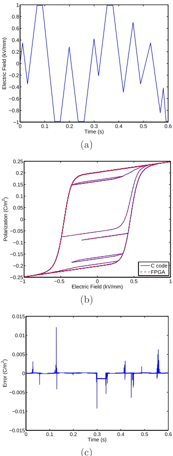
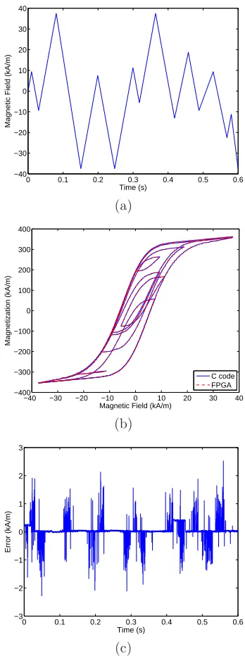
Using parameters obtained from a least squares fit to data from the ferro-electric material PZT yields the model results shown in Figure 3, and Figure 4 gives similar results for parameters obtained from a least squares fit to data from the ferromagnetic material Terfenol-D. Note that in both figures the fields and polarization/magnetization values were scaled to lie in (-1, 1) and the re-sults scaled back to yield the customary units. While some accuracy is lost by the fixed-point arithmetic, it can be seen in the figures that the loss is minor. The PZT example yielded a peak error between the FPGA and floating point C code of 2400 µC/m2 and a root mean square error of 95 µC/m2. For the Terfenol-D example, the peak error was 2526 kA/m and the root mean square error was only 239 kA/m. This is typically much less than other sources of error in the system, and for most applications this loss of accuracy will be more than compensated for by the increased rate at which the model can be run.
4. FPGA Implementation of Thermal Relaxation Model
4.1. Implementation Description
The thermal relaxation model may be formulated by (15) as well, with the difference in the models being the calculation ofx+. As in the negligible
relax-ation case, the input field is assumed to be a 14 bit signed number in (−1,1); the size is determined by the ADC. In this case, however, the field is multiplied byp
V /2kT η×lookup table stepin order to determine the index into the lookup table forposandneg(see [2]). The quadrature pointsEcandEI are multiplied
Throughput Latency Floating point C code – Pentium IV 1.7 GHz 20,000 50,000 Floating point C code – Pentium IV 3.8 GHz 100,000 10,000 FPGA implementation – Virtex II 3000 66 MHz 8,250,000 360 ns
0 0.1 0.2 0.3 0.4 0.5 0.6 −1
−0.8 −0.6 −0.4 −0.2 0 0.2 0.4 0.6 0.8 1
Time (s)
Electric Field (kV/mm)
(a)
−1 −0.5 0 0.5 1
−0.25 −0.2 −0.15 −0.1 −0.05 0 0.05 0.1 0.15 0.2 0.25
Electric Field (kV/mm)
Polarization (C/m
2)
C code FPGA
(b)
0 0.1 0.2 0.3 0.4 0.5 0.6
−0.015 −0.01 −0.005 0 0.005 0.01 0.015
Time (s)
Error (C/m
2)
(c)
0 0.1 0.2 0.3 0.4 0.5 0.6 −40
−30 −20 −10 0 10 20 30 40
Time (s)
Magnetic Field (kA/m)
(a)
−40 −30 −20 −10 0 10 20 30 40
−400 −300 −200 −100 0 100 200 300 400
Magnetic Field (kA/m)
Magnetization (kA/m)
C code FPGA
(b)
0 0.1 0.2 0.3 0.4 0.5 0.6
−3 −2 −1 0 1 2 3
Time (s)
Error (kA/m)
(c)
by the same value before being stored on the FPGA. The lookup table is fixed at 4096 entries between -6 and 25 (with linear interpolation or setting to zero for values outside this range, as discussed in [2]), but the parametersV,T, and
η may vary. To maintain accuracy with this variance, the product is left as a signed, 32 bit number with 4 bits after the binary point for the input field, and unsigned 31 bit numbers with 4 fractional bits forEc andEI. However, to allow both the value and its address to fit into a single 32-bit register, quadra-ture points are input in the 23 bit floating point type described in the next two paragraphs and converted to fixed point on the FPGA.
Computation of the dipole fractionx+ is significantly more complicated in
the thermal relaxation formulation of the model. The erfcx function goes asymptotically to zero as its operand decreases, while it grows nearly linearly for large operands. More than ten orders of magnitude variance in observedpos
and neg is not uncommon. With fixed point arithmetic, this requires a large number of bits to obtain an accurate representation. Moreover, the update for
x+is sensitive to error inposandneg; thus, utilizing only 15 or 20 bits for these
values yields an unacceptable level of error for many applications. Instead, we found it advisable to implement this portion of the relaxation model in floating point arithmetic.
In general, floating point arithmetic utilizes more resources and requires more latency than integer arithmetic, assuming the bit widths are comparable. To minimize the overhead, a 23 bit floating point number system was employed, loosely based on the IEEE 754 floating point standard. One bit was allocated for the sign, 8 for the exponent, and 14 for the mantissa. Exponents were stored as an unsigned integer with an offset of 127, as given by the standard, and the first bit of the mantissa is assumed to be 1 and thus is not stored. This gives 15 significant bits of precision for the floating point number, enough to hold the full precision given by the analog to digital converter plus a couple extra bits to minimize error accrual as calculations are performed. Unlike the IEEE standard, however, support for denormalized numbers as well as INF and NaN support is not included in the floating point operations utilized on the FPGA in order to save FPGA resources.
Only the output of the lookup table forposandnegand the solution to (14) need be computed in floating point. However, the multiplication ofx+×wc[i]×
wi[j] requires roughly the same area in fixed point or floating point, and as such this is also performed in floating point to maintain accuracy. The product is converted to a 31 bit fractional fixed point number before the summation, and the result of the summation was truncated to a 15 bit unsigned number with one bit before the binary point. After the left shift to multiply by 2PR (since
PR= 1), this leaves 13 bits after the binary point, which can be combined with
E/η−PR and reduced to a signed, 14 bit number to return over the DAC.
4.2. Results
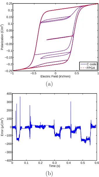
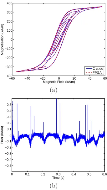
design a throughput of 257,812 timesteps per second. The latency is 5070 ns, and including control logic the design used 66% of the logic resources (slices) on the FPGA. As shown in Table 2, this throughput is over 28 times higher than that achieved by floating point C code on a Pentium IV 1.7 GHz Xeon processor, and 11 times faster than the same C code on a Pentium IV 3.8 GHz Xeon. The latency of the 1.7 GHz Pentium was 21 times slower than the FPGA, and the latency of the 3.8 GHz processor was over 8 times slower. This increase is achieved with very little accuracy lost. Figures 5 and 6 give results parameters representative of PZT and Terfenol-D, respectively. The error introduced in the FPGA by the lower precision arithmetic (interpretted as the difference between the FPGA implementation and a double precision floating point implementation) was less than 368 µC/m2 (peak) or 59 µC/m2 (RMS)
for the PZT example, while the peak error for the Terfenol-D example was less than 369 kA/m and the root mean square error was less than 64 kA/m. As in the negligible relaxation case, these error levels are typically much less than other sources of error in the model, and are acceptable for most applications.
5. Concluding Remarks
Comparing a relatively new, high end Pentium processor to an older, smaller FPGA does not seem equitable; nevertheless we have demonstrated the Virtex II 3000 FPGA was capable of increasing throughput by over an order of mag-nitude compared to a Pentium IV 3.8 GHz processor for both formulations of the model, while the latency was also decreased by almost an order of magni-tude. For the negligible relaxation model, the gap between the computation time of the FPGA and processor was much wider. Using a slower Pentium or embedded microprocessor, the FPGA implementation could easily perform two to three orders of magnitude faster. These savings come with less than 1% loss in accuracy (in reference to the remanence polarization or magnetization), and thus show that FPGAs are an attractive option for model based control of fer-roelectric or ferromagnetic materials. The increased development effort pays a large dividend.
The throughput and latency numbers given in this paper provide a frame-work to determine the size and speed of FPGA needed for a given application.
Throughput Latency Floating point C code – Pentium IV 1.7 GHz 9,200 108,700 Floating point C code – Pentium IV 3.8 GHz 24,000 41,667 FPGA implementation – Virtex II 3000 66 MHz 257,812 5070 ns
−1 −0.5 0 0.5 1 −0.25
−0.2 −0.15 −0.1 −0.05 0 0.05 0.1 0.15 0.2 0.25
Electric Field (kV/mm)
Polarization (C/m
2)
C code FPGA
(a)
0 0.1 0.2 0.3 0.4 0.5 0.6
−400 −300 −200 −100 0 100 200 300 400
Time (s)
Error (
µ
C/m
2)
(b)
Figure 5: (b) Results of the thermal relaxation model for both the FPGA and double precision floating point C code as well as (c) the difference between the codes, which can be interpret-ted as error introduced by the lower precision FPGA calculations. Material parameters are representative for PZT, and the input field can be observed in Figure 3(a).
For example, if offline analysis suggests Nc = NI = 64, then the through-put of the FPGA would be exactly 1/4 of the values presented here for the
−60 −40 −20 0 20 40 60 −400
−300 −200 −100 0 100 200 300 400
Magnetic Field (kA/m)
Magnetization (kA/m)
C code FPGA
(a)
0 0.1 0.2 0.3 0.4 0.5 0.6
−0.5 −0.4 −0.3 −0.2 −0.1 0 0.1 0.2 0.3 0.4 0.5
Time (s)
Error (kA/m)
(b)
Figure 6: (b) Results of the thermal relaxation model for both the FPGA and double precision floating point C code as well as (c) the difference between the codes, which can be interpret-ted as error introduced by the lower precision FPGA calculations. Material parameters are representative for Terfenol-D, and the input field can be observed in Figure 4(a).
the designs discussed in this paper were able to run at 100 MHz instead of 66 MHz, the throughput of both models would have been 50% greater, while the latency would be 50% less.
a slightly higher clock speed would be needed for the relaxation formulation. Such FPGAs are readily available. In short, the capability is present on today’s FPGAs for real-time model based control.
Acknowledgements
This research was supported by a United States Department of Education GAANN fellowship and the Air Force Office of Scientific Research under the grants AFOSR-FA9550-04-1-0203 and AFOSR-FA9550-08-1-0348. The authors also wish to thank Etienne Fiset and Daniel Carbonneau of Lyrtech Signal Processing for their help in procuring and understanding the Lyrtech hardware and software.
References
[1] B.L. Ball, R.C. Smith, S. Kim, and S. Seelecke, “A stress-dependent hys-teresis model for ferroelectric materials,” Journal of Intelligent Material Systems and Structures, 18(1), pp. 69-88, 2007.
[2] T.R. Braun and R.C. Smith, “High speed model implementation and inver-sion techniques for ferroelectric and ferromagnetic transducers,”Journal of Intelligent Material Systems and Structures, 19(11), pp. 1295–1310, 2008.
[3] T.R. Braun and R.C. Smith, “Efficient implementation algorithms for ho-mogenized energy models,” Continuum Mechanics and Thermodynamics, 18(3-4), pp. 137-155, 2006.
[4] T.R. Braun, R.C. Smith, and M.J. Dapino, “Experimental validation of a homogenized energy model for magnetic after-effects,” Applied Physics Letters, 88(12), 2006.
[5] M.J. Dapino, R.C. Smith, L.E. Faidley, and A.B. Flatau, “A coupled structure-magnetic model for magnetostrictive transducers,”Journal of In-telligent Material Systems and Structures, 11(2), pp. 134-152, 2000.
[6] P. Ge and M. Jouaneh, “Modeling hysteresis in piezoceramic actuators,”
Precision Engineering, 17, pp. 211-221, 1995.
[7] D.C. Jiles and D.L. Atherton, “Theory of ferromagnetic hysteresis”, Mag-netism and Magnetic Materials, 61, pp. 1265-1281, 1984.
[8] J.A. Main and E. Garcia, “Design impact of piezoelectric actuator nonlin-earities,”Journal of Guidance, Control and Dynamics, 20(2), pp. 327-332, 1997.
[10] J.A. Main, E. Garcia and D.V. Newton, “Precison position control of piezo-electric actuatorss using charge feedback,” Journal of Guidance, Control, and Dynamics, 18(5), pp. 1068-73, 1995.
[11] J.A. Main, D. Newton, L. Massengil and E. Garcia, “Efficient power ampli-fiers for piezoelectric applications,” Smart Structures and Materials, 5(6), pp. 766-775, 1996.
[12] I.D. Mayergoyz,Mathematical Models of Hysteresis, Springer-Verlag, New York, 1991.
[13] S. Mittal and C-H. Meng, “Hysteresis compensation in electromagnetic actuators through Preisach model inversion,” IEEE/ASME Transactions on Mechatronics, 5(4), pp. 394-409, 2000.
[14] J.M. Nealis and R.C. Smith, “Model-based robust control design for a mag-netostrictive transducer operating in hysterestic and nonlinear regimes,”
IEEE Transactions on Control Systems Technology, 15(1), pp. 22-39, 2007.
[15] W.S. Oates, P. Evans, R.C. Smith, and M.J. Dapino, “Experimental im-plementation of a hybrid nonlinear control design for magnetostrictive ac-tuators,” CRSC Technical Report CRSC-TR06-27; Journal of Dynamic Systems, Measurement, and Control, to appear.
[16] G. Robert, D. Damjanovic and N. Setter, “Preisach modeling of piezo-electric nonlinearity in ferropiezo-electric ceramics,”Journal of Applied Physics, 89(9), pp. 5067-5074, 2001.
[17] R.C. Smith,Smart Material Systems: Model Development, SIAM, Philadel-phia, 2005.
[18] R.C. Smith, M.J. Dapino, T.R. Braun and A.P. Mortensen, “A Homoge-nized energy framework for ferromagnetic hysteresis,” IEEE Transactions on Magnetics, 42(7), pp. 1474-1769, 2006.
[19] R.C. Smith, M.J. Dapino and S. Seelecke, “A free energy model for hys-teresis in magnetostrictive transducers,”Journal of Applied Physics, 93(1), pp.458-466, 2003.
[20] R.C. Smith, A.G. Hatch, T. De, M.V. Salapaka, R.C.H. del Rosario, and J.K. Raye,“Model Development for Atomic Force Microscope Stage Mech-anisms,” SIAM Journal on Applied Mathematics, 66(6), pp. 1998-2026, 2006.
[22] R.C. Smith, S. Seelecke, M.J. Dapino and Z. Ounaies, “A unified framework for modeling hysteresis in ferroic materials,”Journal of the Mechanics and Physics of Solids, 54(1), pp. 46-85, 2006.
[23] R.C. Smith, S. Seelecke, Z. Ounaies and J. Smith, “A free energy model for hysteresis in ferroelectric materials,” Journal of Intelligent Material Systems and Structures, 14(11), pp. 719-739, 2003.
[24] G. Song, J. Zhao, X. Zhou and J.A. Abreu-Garci, “Tracking control of a piezoceramic actuator with hysteresis compensation using inverse Preisach model,” IEEE/ASME Transactions on Mechatronics, 10(2), pp. 198-209, 2005.
[25] X. Tan and O. Bennani, “Fast inverse compensation of Preisach-type hys-teresis operators using field-programmable get arrays,” Proceedings of the American Control Conference, Seattle, WA, pp. 2365–2370, 2008.