Latent Group-Based Interaction Effects in Unreplicated Factorial Experiments.

(1)

ABSTRACT

FRANCK, CHRISTOPHER. Latent Group-Based Interaction Effects in Unreplicated Factorial Experiments. (Under the direction of Dr. Jason Osborne.)

(2)

c

(3)

Latent Group-Based Interaction Effects in Unreplicated Factorial Experiments

by

Christopher Franck

A dissertation submitted to the Graduate Faculty of North Carolina State University

in partial fulfillment of the requirements for the Degree of

Doctor of Philosophy

Statistics

Raleigh, North Carolina 2010

APPROVED BY:

Dr. Sujit Ghosh Dr. David Dickey

Dr. Jeff Thompson Dr. Jason Osborne

(4)

DEDICATION

(5)

BIOGRAPHY

(6)

ACKNOWLEDGEMENTS

I would like to thank everyone who made this work possible. My advisor Jason Os-borne has been a tremendous mentor and friend to me throughout my time in graduate school. David Dickey has always had a kind ear and a wise suggestion. Sujit Ghosh has challenged me to become a better statistician during every phase of my graduate education. Roger Woodard not only taught me how to teach but also helped me realize I love teaching. Pam Arroway has been a source of support whenever things did not go exactly as planned. Golde Holtzman set me on this path with his practical demon-stration of the power of statistics. Bill Hunt has been strong mentor, advocate and friend.

(7)

LIST OF TABLES

Table 2.1 Degrees of freedom for model (1.2) . . . 16

Table 2.2 Degrees of freedom for model (2.1) . . . 16

Table 2.3 Form of each of the intervals under investigation. . . 31

Table 2.4 ANOVA table based on the replicated analysis . . . 34

Table 2.5 Comparison of rejection rates for Tukey’s test and ACMIF. Table counts refer to frequency of rejection of null hypothesis atα= 0.05. Cell percentages are in parentheses. Non-zero off-diagonal counts suggest that nonadditivity is present which is unique to each method. 38 Table 2.6 Non-additivity labels and treatment vectors for each group. The labels describe the above treatment means for the rest of Chapter 3. 44 Table 2.7 Simulation results for additive data. First three columns describe experimental setup. Empirical rejection rates are given for both ACMIF and Tukey’s test for non-additivity atα= 0.05. Results are based on 1,000 MC data sets. The∗ denotes a run significantly differ-ent from actual error rate α = 0.05 (unadjusted p-value=0.00207). Standard error for all proportions presented less than 0.0159. . . . 46

Table 2.8 MSE results for four types of estimators for additive data. First three columns describe experimental setup. Other columns report mean squared error for the various estimators. Results are based on 1,000 MC data sets. . . 47

Table 2.9 Squared bias results for four types of estimators for additive data. First three columns describe experimental setup. Other columns report squared bias for the various estimators. Results are based on 1,000 MC data sets. . . 48

Table 2.10 Variance results for four types of estimators for additive data. First three columns describe experimental setup. Other columns report variance for the various estimators. Notevariance+Bias2 =M SE. Results are based on 1,000 MC data sets. . . 49

(9)

Table 2.12 Simulation results for various latent group non-additive scenarios. Three treatments and seven blocks were used. First two columns describe experimental setup. Third and fourth column provide em-pirical power for ACMIF and Tukey’s test at α= 0.05. McNemar’s test indicates ACMIF different from Tukey’s test for all cases when estimates not equal (p-values<0.0001). Standard error for all pro-portions presented less than 0.0159. . . 54 Table 2.13 MSE results for four types of estimators under various latent group

non-additive scenarios. Three treatments and seven blocks were used. First two columns describe experimental setup. Other columns report mean squared error for the various estimators. . . 55 Table 2.14 Squared bias results for four types of estimators under various latent

group non-additive scenarios. Three treatments and seven blocks were used. First two columns describe experimental setup. Other columns report squared bias for the various estimators. . . 56 Table 2.15 Variance results for four types of estimators under various latent

group non-additive scenarios. Three treatments and seven blocks were used. First two columns describe experimental setup. Other columns report variance of the various estimators. . . 57 Table 2.16 Coverage proportions for four types of intervals under various latent

group non-additive scenarios. Three treatments and seven blocks were used. First two columns describe experimental setup. Remain-ing columns report proportion of MC datasets for which associated confidence interval covers true parameter value. Standard error for all proportions presented less than 0.0159. . . 58 Table 3.1 Data labels and corresponding treatment means for BF simulation

study. . . 79 Table 3.2 Simulation distributional results: relative frequencies of BF

approx-imation appear in columns 2-5. Median BF appears in column 6. Tukey’s test rejection rates (α = 0.05) in additive case appear in the last column. . . 80 Table 3.3 Simulation distributional results: relative frequencies of BF

(10)

Table A.1 Simulation results for various latent group non-additive scenarios. Two treatments and four blocks were used. First two columns de-scribe experimental setup. Third and fourth column provide empir-ical power for ACMIF and Tukey’s test at α = 0.05. McNemar’s test indicates ACMIF is different from Tukey’s test for all cases (p-values < 0.0001). Standard error for all proportions presented less than 0.0159. . . 93 Table A.2 MSE results for four types of estimators under various latent group

non-additive scenarios. Two treatments and four blocks were used. First two columns describe experimental setup. Other columns re-port mean squared error for the various estimators. . . 93 Table A.3 Squared bias results for four types of estimators under various

la-tent group non-additive scenarios. Two treatments and four blocks were used. First two columns describe experimental setup. Other columns report squared bias for the various estimators. . . 94 Table A.4 Variance results for four types of estimators under various latent

group non-additive scenarios. Two treatments and four blocks were used. First two columns describe experimental setup. Other columns report variance of the various estimators. . . 94 Table A.5 Coverage proportions for four types of intervals under various

la-tent group non-additive scenarios. Two treatments and four blocks were used. First two columns describe experimental setup. Remain-ing columns report proportion of MC datasets for which associated confidence interval covers true parameter value. Standard error for all proportions presented less than 0.0159. . . 95 Table A.6 Simulation results for various latent group non-additive scenarios.

Two treatments and seven blocks were used. First two columns describe experimental setup. Third and fourth column provide em-pirical power for ACMIF and Tukey’s test at α= 0.05. McNemar’s test indicates ACMIF different from Tukey’s test for all cases when estimates not equal (p-values<0.0001). Standard error for all pro-portions presented less than 0.0159. . . 95 Table A.7 MSE results for four types of estimators under various latent group

non-additive scenarios. Two treatments and seven blocks were used. First two columns describe experimental setup. Other columns re-port mean squared error for the various estimators. . . 96 Table A.8 Squared bias results for four types of estimators under various

(11)

Table A.9 Variance results for four types of estimators under various latent group non-additive scenarios. Two treatments and seven blocks were used. First two columns describe experimental setup. Other columns report variance of the various estimators. . . 97 Table A.10 Coverage proportions for four types of intervals under various

la-tent group non-additive scenarios. Two treatments and seven blocks were used. First two columns describe experimental setup. Remain-ing columns report proportion of MC datasets for which associated confidence interval covers true parameter value. Standard error for all proportions presented less than 0.0159. . . 97 Table A.11 Simulation results for various latent group non-additive scenarios.

Two treatments and eleven blocks were used. First two columns describe experimental setup. Third and fourth column provide em-pirical power for ACMIF and Tukey’s test at α= 0.05. McNemar’s test indicates ACMIF different from Tukey’s test for all cases when estimates not equal (p-values<0.0001). Standard error for all pro-portions presented less than 0.0159. . . 98 Table A.12 MSE results for four types of estimators under various latent group

non-additive scenarios. Two treatments and eleven blocks were used. First two columns describe experimental setup. Other columns report mean squared error for the various estimators. . . 98 Table A.13 Squared bias results for four types of estimators under various latent

group non-additive scenarios. Two treatments and eleven blocks were used. First two columns describe experimental setup. Other columns report squared bias for the various estimators. . . 99 Table A.14 Variance results for four types of estimators under various latent

group non-additive scenarios. Two treatments and eleven blocks were used. First two columns describe experimental setup. Other columns report variance of the various estimators. . . 99 Table A.15 Coverage proportions for four types of intervals under various latent

(12)

Table A.16 Simulation results for various latent group non-additive scenarios. Three treatments and four blocks were used. First two columns describe experimental setup. Third and fourth column provide em-pirical power for ACMIF and Tukey’s test at α= 0.05. McNemar’s test indicates ACMIF different from Tukey’s test for all cases (p-values < 0.0001). Standard error for all proportions presented less than 0.0159. . . 101 Table A.17 MSE results for four types of estimators under various latent group

non-additive scenarios. Three treatments and four blocks were used. First two columns describe experimental setup. Other columns re-port mean squared error for the various estimators. . . 102 Table A.18 Squared bias results for four types of estimators under various latent

group non-additive scenarios. Three treatments and four blocks were used. First two columns describe experimental setup. Other columns report squared bias for the various estimators. . . 103 Table A.19 Variance results for four types of estimators under various latent

group non-additive scenarios. Three treatments and four blocks were used. First two columns describe experimental setup. Other columns report variance the various estimators. . . 104 Table A.20 Coverage proportions for four types of intervals under various

la-tent group non-additive scenarios. Three treatments and four blocks were used. First two columns describe experimental setup. Remain-ing columns report proportion of MC datasets for which associated confidence interval covers true parameter value. Standard error for all proportions presented less than 0.0159. . . 105 Table A.21 Simulation results for various latent group non-additive scenarios.

Three treatments and eleven blocks were used. First two columns describe experimental setup. Third and fourth column provide em-pirical power for ACMIF and Tukey’s test at α= 0.05. McNemar’s test indicates ACMIF different from Tukey’s test for all cases when estimates not equal (p-values<0.0001). Standard error for all pro-portions presented less than 0.0159. . . 106 Table A.22 MSE results for four types of estimators under various latent group

non-additive scenarios. Three treatments and eleven blocks were used. First two columns describe experimental setup. Other columns report mean squared error for the various estimators. . . 107 Table A.23 Squared bias results for four types of estimators under various latent

(13)

Table A.24 Variance results for four types of estimators under various latent group non-additive scenarios. Three treatments and eleven blocks were used. First two columns describe experimental setup. Other columns report variance of the various estimators. . . 109 Table A.25 Coverage proportions for four types of intervals under various latent

group non-additive scenarios. Three treatments and eleven blocks were used. First two columns describe experimental setup. Remain-ing columns report proportion of MC datasets for which associated confidence interval covers true parameter value. Standard error for all proportions presented less than 0.0159. . . 110 Table A.26 Simulation distributional results for BF approximation and Tukey’s

test rejection rates in cancellatory case. . . 110 Table A.27 Simulation distributional results for BF approximation and Tukey’s

test rejection rates in inert versus active case. . . 111 Table A.28 Simulation distributional results for BF approximation and Tukey’s

(14)

LIST OF FIGURES

Figure 2.1 1000 MC Minimum p-values from additive data with four blocks and three treatments. The histogram of these p-values does not conform to the Beta(1,c) overlay because of the dependency be-tween configurations. . . 21 Figure 2.2 Visual examples of some types of group-based interactions for two

treatments. . . 25 Figure 2.3 Visual examples of some types of group-based interactions for two

treatments. . . 27 Figure 2.4 Visual examples of some types of group-based interactions for three

treatments. . . 28 Figure 2.5 Mean glucose at each combination of storage time and processing

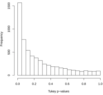
stage. . . 36 Figure 2.6 Histogram of Tukey p-values for each of the 5899 probes for

chro-mosome of interest. The non-uniformity of this plot suggests that non-additivity may be present in these data. . . 39 Figure 2.7 Data from probe 5963 shows non-additivity according to the ACMIF

test but not the Tukey test. Notice the similarity between this pat-tern and the cancellatory patpat-tern in Section 2.1. . . 40 Figure 2.8 Data from probe 1280 shows non-additivity according to the ACMIF

test but not the Tukey test. Notice the similarity between this pat-tern and the inert versus active patpat-tern in Section 2.1. . . 41 Figure 2.9 Power plots for average versus active data for both methods. a =

2, b = {4,7,11}. 1

σ2 plotted on x axis and empirical power at

α= 0.05 plotted on y axis. . . 59 Figure 3.1 Interaction plot. . . 73 Figure 3.2 Interaction plot coded by most likely classification based on a two

component model. . . 74 Figure 3.3 Histograms of univariate data in two component mixtures. First

component is centered at zero and second component is centered at 60. . . 79 Figure 3.4 Histograms of log₁₀(BF) Bayes factors in additive data for N =

300 MC data sets and various levels of σ2_{. . . .} ₈₀

Figure 3.5 Histograms of log₁₀(BF) BF in accordion data for N = 300 MC data sets and various levels ofσ2_{. . . .} ₈₁

(15)

Figure A.2 Power plots for inert versus active data for both methods. a = 2, b={4,7,11}. 1

σ2 plotted on x axis and empirical power atα= 0.05

plotted on y axis. . . 112 Figure A.3 Power plots for cancellatory data for both methods. a = 2, b =

{4,7,11}. 1

σ2 plotted on x axis and empirical power at α = 0.05

plotted on y axis. . . 113 Figure A.4 Power plots for inert versus active data for both methods. a = 3,

b={4,7,11}. 1

σ2 plotted on x axis and empirical power atα= 0.05

plotted on y axis. . . 114 Figure A.5 Power plots for average versus active data for both methods. a =

3, b = {4,7,11}. 1

σ2 plotted on x axis and empirical power at

α= 0.05 plotted on y axis. . . 115 Figure A.6 Power plots for cancellatory data for both methods. a = 3, b =

{4,7,11}. 1

σ2 plotted on x axis and empirical power at α = 0.05

plotted on y axis. . . 116 Figure A.7 Histograms of log10(BF) in cancellatory data for N = 300 MC

data sets and various levels ofσ2_{. . . .} ₁₁₇

Figure A.8 Histograms oflog10(BF) in average versus active data forN = 300

MC data sets and various levels of σ2. . . 118 Figure A.9 Histograms oflog10(BF) inert versus active data forN = 300 MC

(16)

Chapter 1 Introduction

1.1 Background

(17)

the other factor may affect the response differently in each of these groups. We allow the groupings of one of the factor levels to interact with the other factor. For instance per-haps all varieties of some crop perform equivalently in poor soil but some of the varieties flourish more than others in fertile soil.

To illustrate the above idea using randomized complete block design (RCBD) terminol-ogy, imagine that we conduct such a study under the assumption that treatments do not interact with blocks. Upon collecting the data we begin to suspect that the blocks are possibly members of some smaller number of latent groups, or environments, and these groups interact with the treatments. We want to develop methods which can formally address whether or not such a latent structure is plausible, and if so, we want to conduct statistical inference with this structure in mind.

(18)

Suppose now that the patients in this population (and hence sample) are heterogenous in some unknown way. Perhaps the treatment affects different people differently based on some genetic trait. Some patients have this trait and the rest do not, so in this case there are two groups from which the patients arise. If the number of groups and patient membership within these groups are known a priori then standard linear modeling tech-niques will allow us to assess treatment effects, group effects, and interaction between these two factors. Additionally, the additive variability between patients within groups can be modeled. A full discussion of the merits and caveats of the group based model is included in Chapter 2.

Replication is a principle of sound experimental design for scientific experimentation. It seems unlikely that any single statistical method will arise that will be totally satisfactory to detect all types of interaction effects in unreplicated experiments. In lieu of a silver bullet method a number of methods have been proposed to detect and perform inference on restricted interaction parameter models. Many such models and methods have arisen. However the physical interpretation of many of the restricted interaction models in terms of real world phenomena is possibly non-intuitive for many cases. Methods based on the latent group restriction can be intuitive in situations where a grouping structure is sen-sible.

(19)

Before elaborating on our methods we first review the basic problem and available litera-ture more fully. Consider the balanced two-way analysis of variance (ANOVA) model for independent response variables yijm observed in a completely randomized experiment:

yijm =µ+αi+βj + (αβ)ij +ijm . (1.1)

where i = 1, .., a > 1 is an index for the levels of one of the two factors, j = 1, ...b > 1 indexes the levels of the other factor, and m = 1, ..., n > 1 is an index for the number of replicates for experimental units, ijm ∼ N(0, σ2). Note αi, βj, and (αβ)ij may be

either fixed or random effects depending on the nature of the study. In the fixed effect case we adopt the sum-to-zero parameterization (e.g., Pa

i=1αi = 0). For random effects

we assume normality (e.g., αi iid

∼ N(0, γ2) for i = 1, ..., a. In this scenario all parame-ters are estimable and statistical inference can be performed using the two-way ANOVA technique. However, for the the special case where m = 1 the there is no error-variance estimate to use in the denominator for the usual F tests for model parameters.

The RCBD is a well known example of a two way unreplicated factorial design. The following additive model is commonly posited for RCBDs:

yij =µ+αi+βj+ij . (1.2)

where i = 1, .., a;j = 1, ...b;Pa

i=1αi = 0;βj ∼ N(0, σB2);ij ∼ N(0, σ2). Typically the

treatment effects (denotedαi) are considered fixed and the block effects (denotedβj) are

(20)

Choice of an unreplicated design does not preclude the possibility that the factors truly have non-zero interaction effects. Since ignoring important model terms leads to biased estimation, we are interested in investigating alternative (but necessarily more restric-tive) forms of interaction effects to those described in model (1.1).

We will propose two methods to diagnose nonadditivity in unreplicated experiments. In this thesis we focus mainly on the one versus two group question although investigation of a greater number of groups is generally of interest. The first method considers all pos-sible groupings of blocks into two groups and in doing so determines whether the optimal configuration exhibits significant group by treatment interaction while adjusting for the multiplicity of the large number of possible configurations. We present a model based on this configuration which can accommodate treatment effect, group effect, treatment by group interaction, and also additive block variability. Blocks are nested in groups in this case. Our review of restricted interaction parameter models illustrates historical developments for this problem while also demonstrating the difference between existing methods and the all configurations approach.

(21)

We now review current models and methods for addressing non-additivity in unreplicated factorial experiments.

1.2 Non-additivity in Unreplicated Experiments

Perhaps the first formal investigation of non-additivity in unreplicated experiments is the one degree of freedom test for non-additivity proposed by Tukey (1949). In the original paper no model is explicitly defined, however it has been pointed out (Alin and Kurt, 2006) that the test is based on the following model:

yij =µ+αi+βj +ναiβj+ij . (1.3)

It is clear that this model includes a single ν parameter in addition to those in (1.2). A test of non-additivity can then be defined in terms of hypotheses H0 : ν = 0 versus

H1 :ν 6= 0. The ANOVA table for this test is similar to the ANOVA table for the

(22)

fundamental feature of the data. The model (1.3) will henceforth be referred to as the ‘Tukey Model.’ Tukey (1955) explains how to apply this method to larger experiments.

Mandel (1961) developed a generalization of Tukey’s model.

yij =µ+αi+βj +θjαi+ij . (1.4)

where i= 1, ..., a >2;j = 1, ..., b. Mandel’s interaction parameters are essentially block-specific constants multiplied with the treatment main effects. This model has been called the “rows-linear model” by Alin and Kurt (2006). Instead of adding one interaction pa-rameter as in the Tukey model, Mandel allows (b−1) parameters for interaction. Note that if a= 2 then there are not enough degrees of freedom to accommodate this form of interaction after accounting for block, treatment, and error terms.

To see the linear expression, defineQj = (θj+ 1) and letµj =µ+βj. Now for any given

level of j, Mandel’s model can be expressed as:

yij =µj+αiQj +ij . (1.5)

That is, each observation can be characterized as a block-specific intercept plus a treat-ment effect times a block-specific constant plus some random error.

Ten years after publishing the previous model, Mandel (1971) put forth another model for non-additive effects:

(23)

whereηij =PQ_q₌₁θqUqiνqj., Q≤min(a−1, b−1). Both the value ofQand the estimates

of parameters θq, Uqi, νqj. are determined according to features of the spectral

decompo-sition of DDT_{, where} _D _{is the matrix of residuals from the additive model defined by}

dij =yij −µb−αbi−βbj. The hat terms are the usual least squares estimators.

The motivation of this model is that αi and βj account for all additive variability in the

response, and the termηij is some combination of interaction effects plus random

variabil-ity (to distinguish fromij which denotes only random error). The parametersθq, Uqi, νqj.

are estimated using the matrix DDT_{, which has} _{min(a, b) real eigenvalues with}

orthog-onal eigenvectors. If the full decomposition is performed there will be no terms left for residual error which leads to the restriction Q≤min(a−1, b−1). Mandel recommends choosing Q so that only a few multiplicative interaction terms are included, combining the rest of the decomposition terms into residual error. Note that the estimates ˆθq for

q = 1, ..., Q are the eigenvalues ofDDT. If there are no positive eigenvalues, then (1.6) reduces to the additive case. So testing the hypothesis θq = 0∀q = 1, ..., Q is analogous

to testing for the presence of non-additivity by determining if any of the eigenvalues of DDT _{differ significantly from zero. This eigenvalue decomposition strategy is}

sim-ilar to the Factor Analysis of Variance (FANOVA) technique illustrated by Gollob (1968).

(24)

components ofA×B,A×C,B×C, and the linear×linear×linear components ofA×B×C. The model for the p= 3 case is as follows:

yijk =µ+αi+βj +νk+δ1αiβj +δ2αiνk+δ3βjνk+δ4αiβjνk . (1.7)

where Pa

i=1αi =

Pb

j=1βj =

Pd

k=1νk =

Pa

i=1

Pb

j=1αiβj =

Pa

i=1

Pd

k=1αiνk=

Pb

j=1

Pd

k=1νkβj =

Pa

i=1

Pb

j=1

Pd

k=1αiβjνk = 0. Notice that if p= 2 this is identical to

the Tukey Model.

Pardo and Pardo (2005) address the analogous case of non-additivity in log-linear models for count data. This addresses multinomial, product multinomial, and Poisson sampling schemes. They develop test statistics to diagnose non-additivity using φ-divergences, which include Kullback-Leibler divergence as a special case.

Johnson and Graybill (1972a) introduced a model to assess interaction in unreplicated experiments. Their model is as follows:

yij =µ+αi+βj +λτiγj+ij . (1.8)

where Pa i αi =

Pb jβj =

Pa i τi =

Pb

jγj = 0,

Pa i τ 2 i = Pb jγ 2

j = 1, and ijm ∼ N(0, σ2).

(25)

normalized eigenvector corresponding to the largest eigenvalues of the outer and inner products of the a×b matrix of residuals respectively. The parameter λ is estimated by the largest eigenvalue of the inner product of the a×b matrix of residuals. Johnson and Graybill develop a corresponding LR test (LRT) of H0 : λ = 0 versusH1 :λ 6= 0 based

on their model, and suggest that it may be better than Tukey’s and related tests in cases where the true form of the interaction is not a function of the treatment and block effects. This model is a specific case of (1.6) with Q= 1.

Estimation of error variance in non-additive models with unreplicated data is not straight-forward. Nonadditivity between treatment and block effects will lead to inflated error variance estimation when the additive model(1.2) is used to estimate σ2_{. One way to}

approach this problem is given by Johnson and Graybill (1972b). The authors decompose the uniformly minimum variance unbiased estimate (UMVUE) for σ2 into a number of squared two by two contrasts. The authors then argue that the effects of the factors on the response is additive if and only if the mean of each of the two-by-two contrasts is zero. Some distributional theory is provided for various functions of the eigenvalues from residual matrices, which ultimately lead to a procedure for determining if these contrasts are significantly larger than we would expect under additivity. Each of these contrasts is compared to a cutoffCα, and the probability that one of these contrasts exceedsCαunder

additivity is smaller than the preassigned α level. The proposed estimator of variance is then based on only the two by two contrasts which do not differ significantly from zero. If no contrasts exceed Cα then their estimate of variance is equivalent to the UMVUE

(26)

Barker et al. (2009) develop the orthogonal interaction model (OIM) for unreplicated ex-periments. Rather than restricting the form of the interaction to some type of multiplica-tive setup, interactions and main effects are constrained to be orthogonal. This model may be used in two-way factorial designs whether or not replication is present. Starting with the original two-way model (1.1), the additional constraints Pa

i=1αi(αβ)ij = 0∀i,

and Pb

j=1βj(αβ)ij = 0∀j are imposed which implies that main effects and interactions

are orthogonal. Barker develops a remeasurement process in order to assign degrees of freedom for the purpose of testing for effects.

The common strategy in the above cases is to develop a restricted form of interaction model. The various models retain main effects and borrow degrees of freedom from the error term. Over time the models have escalated in complexity. In practice one may not know which of the available methods most accurately captures interaction present in a given data set. In the literature, competing methods are generally compared in terms of statistical power for various forms of non-additivity.

1.3 Component Number Selection for Finite

Mix-ture Models

(27)

component multivariate mixture:

f(y|θ) =ωf1(y|θ1) + (1−ω)f2(y|θ2) . (1.9)

where θ = (θ1,θ2), 0 ≤ ω ≤ 1. If ω = {0,1} or θ1 = θ2, then the above expression

reduces to a one component model. It is clear that ω can be defined on the boundary of its parameter space, which is problematic for a variety of standard statistical procedures. For instance the standard asymptotic properties of the likelihood ratio test (LRT) statis-tic require that the parameter space contain an open set, and the true parameter be an interior point of this set (see e.g. Casella and Berger (2002)). Since this condition does not hold the LRT statistic does not enjoy its usual asymptotic properties under the null hypothesis. In the univariate case Ghosh and Sen (1984) derived the asymptotic distri-bution of the LRT statistic in the g = 1 versus g = 2 case under a separation condition |µ2−µ1| > > 0, where µ1 and µ2 are the location parameters for each component in

the mixture.

A more recent paper by Garel (1996) allows the relaxation of this condition in the uni-variate case. This paper also focuses on the d = 1 versus d = 2 problem due to the adequacy of available theoretical results in this case. Garel notes that testing a differ-ence of more than one component requires nonstationary random fields for which there is a comparative dearth of available results. This technical paper highlights the difficult theory needed for this problem.

(28)

mea-sures the likelihood achieved by a candidate model with a penalty attached for the num-ber of parameters in that model. Both criteria have been used by researchers for the component number selection problem, but Titterington et al. (1985) point out that the regularity conditions for these criteria are also violated since the parameter ω can exist on the edge of the parameter space. Hence, the asymptotic justification for these two criteria is invalid, though both have been used for our purpose in scientific literature.

Bayesian methodologies have been developed to address this issue as well. The deviance information criterion (DIC) was first developed by Spiegelhalter et al. (2002). DIC was designed in a general framework to compare hierarchical models when the number of pa-rameters is unknown. Celeux et al. (2006) focus the potential of the DIC on estimating the number of components in mixture models. Since various model specifications may be of interest in this context, Celeux et al. (2006) explore 8 different parameterizations of DIC in the paper.

(29)

(30)

Chapter 2 All Configurations Approaches

Our methods for assessing non additivity diverge from many existing techniques. We focus on determining if the levels of one of the predictors fall into some smaller number of latent groups. If this latent grouping structure exists and is known in advance the following model would be appropriate:

yij(k) =µ+αi+ξk+ (αξ)ik+βj(k)+ij(k) . (2.1)

where i= 1, .., a;j = 1, ...b;k = 1, ..., g;g < b. The treatment effects are denotedαi, the

group effects are denotedξk, the treatment by group interaction parameters are denoted

(αξ)ik, the block effects are denoted βj(k), and the error terms are denoted ij(k). The

following constraints Pa

i=1αi =

Pg

k=1ξk =

Pa

i=1(αξ)ik =

Pg

k=1(αξ)ik = 0 hold. Also

βj(k) ∼N(0, σB2); ij(k) ∼ N(0, σ2). Model (2.1) accommodates the full set of treatment

(31)

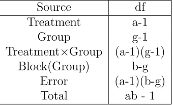
Table 2.1: Degrees of freedom for model (1.2)

Source df

Treatment a-1

Block b-1

Error (a-1)(b-1) Total ab - 1

Table 2.2: Degrees of freedom for model (2.1)

Source df

Treatment a-1

Group g-1

Treatment×Group (a-1)(g-1) Block(Group) b-g

Error (a-1)(b-g)

Total ab - 1

we maintain the traditional notion that blocks are heterogeneous but add the assumption that they belong to some smaller (but possibly unknown) number of groups. Within each group the treatment effects are constant, but the treatment effects may be different in the different groups. We can now assess the interaction between these groups and the treatment variable. If treatment by group interaction is present then we are interested in assessing the simple effect of the treatments separately within each group.

Notice that the above model (2.1) can be implemented for any g < b. The available degrees of freedom for this model are summarized in Table 2.2.

(32)

apparent that the group model partitions the block and error sum of squares from the additive model into the group, treatment by group, block(group), and error terms above. Notice that the degree of freedom entries for these terms sum to a(b−1) which equals the sum of the block and error df from the ANOVA table from the additive model (1.2).

One important feature of the group-based model analysis is that the treatment by group interaction test is equivalent to the F test for comparing nested models. In this case we are comparing the group-based model to the additive model. Regard model (2.1) as the full model and (1.2) as the reduced model and define the F statistic in the usual way:

F = (SS(E)Reduced−SS(E)F ull)/(df EF ull−df EReduced) M S(E)F ull

. (2.2)

where

F H0

∼ Fdf EF ull−df EReduced,df EF ull .

Model (2.1) partitions the error sum of squares from the additive model into two parts: SS(E)Reduced =SS(E)F ull+SS(T reatment×Group) so the difference in sum of squares

in the numerator of (2.2) (SS(E)Reduced−SS(E)F ull) = SS(T reatment×Group) where

(T reatment×Group) stands for treatment by group interaction. Also notice the treat-ment by group term has (a−1)(g−1) degrees of freedom, and the difference in degrees of freedom in the numerator of (2.2) (df EF ull−df EReduced) = (a−1)(b−1)−(a−1)(b−g) =

(a−1)(g−1), which is also the number of degrees of freedom from the treatment by group term in model (2.1). Finally, the proper denominator for the treatment by group term is M S(E)F ull. Hence a test of treatment by group interaction in the group model is

(33)

Before implementing the above analysis we want to detect whether or not the described grouping structure plausibly exists. As such we are interested in methods which can help us decide whether the simpler model (1.2) is sufficient, or whether we should favor model (2.1). This question is complicated by the fact that block membership in the groups is unknown and must be treated as a latent variable. Hence two questions arise. First, is it plausible that such a grouping structure exists? If so, how does one conduct inference in light of these features?

One of the methods we have investigated for this purpose is called the all configurations maximum interaction F test (ACMIF). The “all configurations” label implies that we will consider every single possible grouping of blocks for some number of groups. We will use the maximum of all of the interaction F tests among all possible groupings as a criterion. The goal is to determine whether or not a grouping structure plausibly exists. We wish to develop a test which will incorrectly conclude that there is a latent grouping structure when in fact there is none with some preassigned level of significance. Once we have established a level α test we are interested in comparing the power of this method with some other available methods for various alternatives. We continue to use the letterg to denote the number of groups which are present, and we focus on the following hypotheses:

H0 :g = 1, i.e. blocks all belong to the same group. Additive model is sufficient.

H1 :g = 2, i.e. blocks belong to two groups. Effects of the other factor on response vary

across these groups.

(34)

case is consistent with many current papers in the literature such as Garel (1996). In the g = 2 case, there are c= 2(b−1)₋_{1 possible groupings of blocks such that neither group}

is empty. We refer to the set of possible groupings as “configurations.”

In the g = 2 case we want to count all the unique ways in which the blocks may be put into two non-empty groups. There are 2b ways of placing blocks into two groups. Notice this is the standard ordered sampling with replacement formula. We wish to eliminate the configurations where all blocks are contained in one (or the other) group. This leaves us with 2b₋_{2 such groupings. Notice that half of these configurations are duplicate since}

the group label is arbitrary. For example the case where the first block is in the first group and the other blocks are in the second group is identical to the case where the first block is in the second group and all of the other blocks are in the first group. The grouping of which blocks are together is what is important and the group label is irrelevant. So we must divide the above expression by two which leaves the formula c= 2b−1−1 possible configurations.

The all configurations framework has unique features and challenges. For instance, statis-tics which arise from the configurations are not independent. In the context of linear models the null distributions of many statistics are known. However, the joint distri-bution of many of these same statistics over all configurations is not immediately clear. This precludes the use of several convenient strategies available for independent data, including convenient order statistic results for independent samples.

(35)

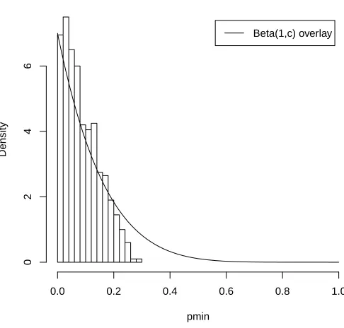
would be an intuitive statistic to examine. After all, we are naively choosing to inves-tigate every possible configuration of blocks and so the configuration with the lowest p-value would seem to correspond to the configuration which holds the most evidence for the existence of g = 2 latent groups. If thec such p-values from all configurations were independent, then the null distribution of the minimum would beBeta(1, c). It would be straightforward to develop a critical value for a levelαtest based on this null distribution and render a decision by comparing the minimum interaction p-value for a given data set to this cutoff. Unfortunately simulations indicate that the distribution of the minimum p-value is not well approximated by a Beta(1, c) distribution. General distributional results for this minimum p-value given the dependency between the configurations are more difficult to derive than in the independent case and have remained elusive.

(36)

Minimum p−value − 1000 additive data sets

pmin

Density

0.0 0.2 0.4 0.6 0.8 1.0

0246

Beta(1,c) overlay

(37)

Our most promising all configurations strategy is to investigate the minimum of all in-teraction p-values and perform a Bonferroni adjustment based on the c configurations. For even modest sized experiments the issue of multiplicity arises since the number of configurations c increases rapidly as a function of the number of blocks. If each of thec interaction p-values is judged againstα then the probability of avoiding all type I errors is bigger than 1−α since many p-values are under simultaneous assessment.

The Bonferroni adjustment is made by splitting the α region into c equally sized parts. To motivate the Bonferroni adjustment, for any events Av, P(Tc_v₌₁Av) ≤ Pc_v₌₁P(Av).

Let us defineAv as the event where we reject the null hypothesis associated with thevth

treatment by group interaction F test when there is no latent grouping structure. By comparing pv to α_c we have bounded the probability of Av above by α_c for v = 1, ..., c.

Hence P(Tc

v=1Av) ≤

Pc

v=1P(Av) =

Pc

v=1 α

c = α. The probability of wrongly

reject-ing any of the Treatment×Group interaction F tests at the α

c cutoff is less than α for

v = 1, ..., c. Alternatively one can multiply a raw p-value by c and compare this Bon-ferroni adjusted p-value with α directly. We will assess power under various alternatives in Section 2.6. Unless specifically stated otherwise, we refer to the Bonferroni adjusted maximum interaction F criteria as ACMIF from now on.

By replacing α with α_c when calculating the cutoff from the null distribution we ensure that P(rejecting any test|H0 true)< α even though these p-values are not independent.

(38)

dom test for several latent group-based interaction scenarios.

To apply the Bonferroni adjustment to the ACMIF test let F1, ..., Fc represent the c

Treatment×Group interaction effects corresponding to all possible configurations, and let F(1), ..., F(c)represent the corresponding order statistics such thatF(1) < F(2) < ... < F(c).

These F statistics are each on (a−1)(g−1) numerator degrees of freedom and (a−1)(b−g) denominator degrees of freedom. Each of these F statistics yields a p-value. Denote these ordered p-values p(1), .., p(c). Then F(c) corresponds to p(1). If the null hypothesis

is true then there is no environmental structure whatsoever in the data. In this case F1, ..., Fc

id

∼F(a−1)(g−1),(a−1)(b−g). Notice these are identically distributed but not

indepen-dent random variables.

Once all of the p-values are computed the strategy is to compare p(1) to α_c. If p(1) < α_c

then reject H0 :g = 1. Otherwise fail to reject H0. This testing procedure maintains a

type I error rate α due to the Bonferroni correction.

2.1 Types of group-based interaction

Many of the existing methods to detect nonadditivity in unreplicated experiments as-sume a form of interaction based on an accompanying model. Clearly the power of any of these tests would seem to be higher for data which exhibits non-additivity of the spec-ified form, and possibly lower for non-additivity of a different form.

(39)

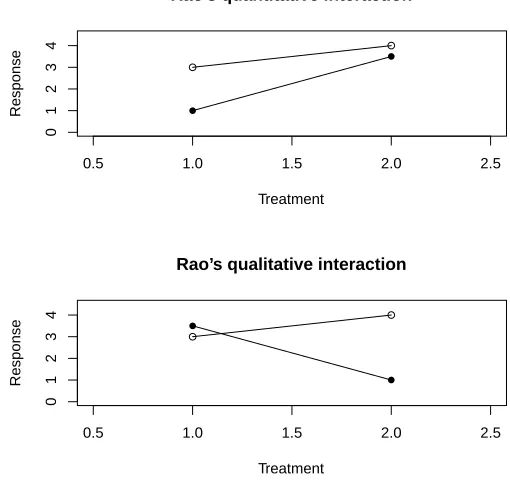
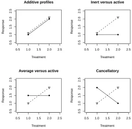
are an infinite number of ways to draw a line on a Cartesian plane. There are also a number of ways to subdivide this broad class of possibilities. For instance Rao (1998) uses interaction plots to characterize interaction in 2×2 experiments as either quantitative if the treatment effects at a given level of the other factor have the same sign slope, or qualitative if the treatment effects at the levels of the other factor have opposite sign slopes. In our case the other factor is the group. Figure 2.2 shows these two types of interaction. Since most of the current methods to detect non-additivity focus on specific subclasses of interaction it is desirable to classify various non-additive forms by the type of method which can detect them. Methods which assume a restricted interaction parameterization perform best for data that exhibits interaction consistent with the restrictions. For our methods latent group based interactions are the non-additive form of interest. We are interested in investigating any type of non-additivity that can be explained by the existence of latent groups which contain the blocks. With this in mind we now turn the discussion to some forms of non-additivity which can be characterized by our group based interactions. While the types of latent group based interaction discussed herein are not a comprehensive list, they demonstrate the breadth of scenarios which fall under the class of latent group interactions.

(40)

0.5 1.0 1.5 2.0 2.5

01234

Rao’s quantitative interaction

Treatment

Response

0.5 1.0 1.5 2.0 2.5

01234

Rao’s qualitative interaction

Treatment

Response

(41)

if one group of patients respond to the treatments, while another group does not. The groupings may be due to some unknown genetic difference between patients. The lower left panel illustrates a similar situation where the inert group is replaced by an “aver-age” group. Even though these most recent panels are similar in some ways, we will see that detection of this type of crossing profile is more problematic for some methods than others. The lower right panel illustrates a form of non-additivity we call “cancellatory”. In this setting the optimal treatments for the two groups are opposite. This situation may arise in learning tasks where the two groups are composed of people with different learning styles.

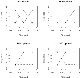
The forms of interaction for the a= 2 case are also of interest for a >2. As the number of treatment levels grow other forms of group based interaction become possible. Figure (2.4) illustrates some interesting possible forms of interaction in the a = 3 treatment case. The “one optimal” and “two optimal” types may occur if some type of intervention is successful on some subset of a population. The “accordion” pattern is an extreme case of crisscrossing profiles. The “different optimal” pattern may occur if different subsets of the population have an increased response for different treatments.

2.2 Statistical inference in the all configurations

frame-work

(42)

0.5 1.0 1.5 2.0 2.5

0.5

1.0

1.5

2.0

2.5

Additive profiles

Treatment

Response

0.5 1.0 1.5 2.0 2.5

0.5

1.0

1.5

2.0

2.5

Inert versus active

Treatment

Response

0.5 1.0 1.5 2.0 2.5

0.5

1.0

1.5

2.0

2.5

Average versus active

Treatment

Response

0.5 1.0 1.5 2.0 2.5

0.5

1.0

1.5

2.0

2.5

Cancellatory

Treatment

Response

(43)

0.5 1.5 2.5 3.5

0.5

1.5

2.5

3.5

Accordian

Treatment

Response

0.5 1.5 2.5 3.5

0.5

1.5

2.5

3.5

One optimal

Treatment

Response

0.5 1.5 2.5 3.5

0.5

1.5

2.5

3.5

Two optimal

Treatment

Response

0.5 1.5 2.5 3.5

0.5

1.5

2.5

3.5

Diff optimal

Treatment

Response

(44)

favor either the notion that there is no latent group structure (i.e. g = 1), or we will come to believe that there are two latent groups (g = 2) which contain the blocks, and this group effect plausibly interacts with the treatment effect. Development of an estimator under model uncertainty is the goal.

Suppose we are interested in assessing the difference in treatment levels i and i0. If we know the null hypothesisH0 :g = 1 is true we estimate the difference in these treatment

levels using the additive model (1.2). Denote this estimator ˜γ and note

˜

γ = ¯yi0_.−y¯_i. . (2.3)

Now suppose we know that the alternative hypothesis H1 : g = 2 is true. If this is the

case then we would like to adjust our inference techniques to reflect our belief that latent groups exist and interact with the treatments. In the presence of treatment by group interaction we are interested in assessing the difference in means across treatment levels i and i0 for a specific groupk. Some authors refer to this contrast of means across levels of one factor while a second factor is held fixed as a simple factorial effect. Let

γ =αi0 −α_i+ (αξ)_i0_k−(αξ)_ik . (2.4)

Estimation of the parameters in (2.4) is not trivial. Even with a priori knowledge that H1 is true, the membership of the blocks in the groups remains a latent variable. In this

manuscript we will explore use of the configuration prescribed by the ACMIF procedure. We will use the configuration of blocks which corresponds to F(c). In other words, we

will take the grouping of blocks which provides the most evidence in favor of H1 and use

(45)

in this fashion. For example ˘γ is the least squares estimator of the following expression:

γ =αi0 −α_i+ (αξ)_i0_k−(αξ)_ik . (2.5)

If we know which hypothesis is true in advance then we have proposed a strategy to estimate the difference in treatment means between treatment i and i0. In practice we need to perform a hypothesis test in order to determine whether H0 orH1 is preferable.

We will suggest an estimator that uses the results from the ACMIF procedure to estimate γ:

γ∗ =   

˜

γ if p(1) > α_c

˘ γ else

. (2.6)

Noteγ∗ takes the value of the appropriate estimator of γ from either the additive model or the group-based model depending on the decision we arrive at using the ACMIF. If we conclude that g = 1 then γ∗ takes the value prescribed by the additive model (1.2). If we reject the null hypothesisH0 : g = 1 thenγ∗ is an estimator based on model (2.1).

The final estimator we will investigate is the least conventional. We wish to consider an estimator which is a weighted average of ˜γ and ˘γ. The weight should be chosen using some measure of evidence of one model versus the other. Consider

˙

γ =p(1)γ˜+ (1−p(1))˘γ . (2.7)

We wish to emphasize that for ˙γ we are not justifying the use ofp(1) based on its

(46)

Table 2.3: Form of each of the intervals under investigation.

Interval Formula

˜

γ interval γ˜±t(a−1)(b−1)×SE(˜γ)

˘

γ interval γ˘±t(a−1)(b−g)×SE(˘γ)

γ∗ interval γ˜ or ˘γ interval as chosen by ACMIF γ∗ ±max(M OE) γ∗±max(M OE(˜γ), M OE(˘γ))

˙

γ interval γ˙ ±t(a−1)(b−g)U B(SE( ˙γ))

assumptions) are true. In the frequentist paradigm a p-value should never be interpreted as the probability that the null hypothesis is true. Our justification for usingp(1) is that

it will be small if the alternative hypothesis is true but larger if the null hypothesis is true. In this way we use it as a convenient weight. We will comment on the performance of ˜γ, ˘γ, γ∗,and ˙γ in terms of mean squared error (MSE) in Section 2.6.

In addition to the point estimators ˜γ, ˘γ, γ∗, and ˙γ we are interested in assessing the performance of various confidence intervals based on these estimators. In our simulation study we will investigate the coverage of four types of intervals: One interval from the additive model, an interval based onγ∗using either the additive interval or group interval as chosen by γ∗, an interval based onγ∗ using the wider margin of error from either ˜γ or ˘

γ, and an interval based on ˙γ.

(47)

of the first two intervals is chosen by the ACMIF method. The γ∗ ±max(M OE) in-terval uses the γ∗ estimator but chooses the wider margin of error between additive and group intervals. The idea here is to account for model uncertainty due to the estimated number of groups based on ACMIF by using a wider interval. Let U B = q

p2

(1)×V ar(˜d γ) + (1−p 2

(1))×V ar(˘d γ) + 2p(1)(1−p(1))V ar(˜d γ)V ar(˘d γ). U B is an upper

bound for the standard error of ˙γ since in general Cov(˜γ,˘γ) ≤ SE(˜γ)∗SE(˘γ). Notice that between using an upper bound for the standard error of ˙γ and the more conservative t(a−1)(b−g)critical value we may expect the length of this latter interval to be greater than

the others. We will compare the performance of several of these intervals in Section 2.6.

Other methods to estimate block membership in groups include clustering and mixture model methods. Instead of choosing the most significant grouping we could also explore standard clustering techniques. It would seem that any technique for assigning blocks to groups will be as successful as its ability to incorporate the group by treatment inter-action into the clustering algorithm. In the mixture model framework we could regard the random vector of data yj arising from block j as a draw from a two component

multivariate normal mixture mixture model. The two components in this mixture model represent the two groups which contain the blocks. We could then model the probability that a given block j arises from the kth component using the following formula

P(block j belongs to group k) = ωfi(yj|θk)

ωf1(yj|θ1) + (1−ω)f2(yj|θ2)

. (2.8)

where 0 < ω < 1 is a mixing weight, ω > (1−ω), fi represents the component density

for group i which is multivariate normal in this case, and θi is the vector of parameters

(48)

vector and covariance matrix. Mixture model notation will be more formally defined and discussed in Chapter 3. Assigning eachyj into its most probable component according to

(2.8) is equivalent to the Bayes rule for assigning i.i.d. data into components (McLachlan and Peel, 2000). One way to approximate this rule is to replace the parameters ω and θk for k = 1,2 in (2.8) with suitable estimates. A ‘most probable’ assignment can be

made by placing each block in whichever group has a higher estimated probability of membership.

One drawback of the mixture model approach described here is that mixture models typically require a fairly large number of observations in order for the model fit to be adequate. The ACMIF method was designed to be effective with a class of experiments that is probably too small to benefit from mixture theory. Nonetheless, a most probable configuration based on mixture model assignment remains as an interesting avenue for future research. We comment on the empirical performance of theγ∗ estimator in section 2.6

2.3 Illustrative example - Sweetpotatoes

(49)

Table 2.4: ANOVA table based on the replicated analysis Source df SS MS F p-value

Time 2 16.6 8.3 40.8 <0.0001 Stage 3 23.1 7.7 37.8 <0.0001 Time*Stage 6 6.3 1.0 5.1 0.0007

Error 36 7.3 0.2 -

-Total 47 53.3 - -

-each of the processing steps all 40 potatoes were processed, and a fixed amount of potato was taken from this total amount of material at each step for glucose testing. The first step is the raw potatoes. For the second processing step each group was cut into strips, blanched and dehydrated. Glucose measurements were taken on a portion of the dehy-drated potato strips from each group. Then the remaining strips were parcooked and another portion of the strips from each group was measured for glucose. Parcook stands for “partial cook.” Frozen french fries from the grocery store are in the parcooked stage. Finally the remaining strips of each group were fried to finish the processing. Glucose measurements were immediately taken on the finished French fries. This is an example of a replicated crossed two way factorial experiment. In this case it is possible to estimate the full complement of interaction parameters. The ANOVA table based on model (1.1) is portrayed in Table 2.4.

Based on the standard two way model there is strong evidence that interaction is present between Time and Stage judging by the small p-value (0.0007).

(50)

this approach are manifold. First, since this data set truly has replication and we have used the two way model (1.1) to establish interaction using standard ANOVA techniques, we can see if our method is able to detect this interaction based on the more crude cell mean data. Second, the most significant grouping established by our method lends credi-ble interpretation to the experimental phenomenon: We will see that the most significant configuration puts raw potatoes in one group and all three processed stages in the other. Third and perhaps most importantly, this example illustrates how our method may be useful in situations where the data arise from an experiment where subsampling was implemented in place of true replication. Statisticians who collaborate with researchers outside the field of statistics sometimes encounter experiments where subsampling was mistakenly used in place of true replication. In a case such as this, one can regard cell means of subsampled units as single observations in an unreplicated experiment and ap-ply the techniques described herein

(51)

of possible interaction the Tukey single degree of freedom test for non-additivity does not provide strong evidence of an interaction effect in this case (p-value = 0.16).

The all configurations maximum interaction F based on thec= 7 runs of model (2.1) is 60.8 on two numerator degrees of freedom and four denominator degrees of freedom. This leads to an unadjusted p-value = 0.0010. The Bonferroni adjusted p-value based on the c= 7 configurations is 0.0070, so at α= 0.05 we reject the null hypothesis of no grouping structure and instead favor the alternative. The most significant configuration places raw potatoes into one group and the other three post-processed types of potatoes into the other group. Our naive method of looking at all possible configurations of treatments into groups has yielded a grouping which corroborates the visual evidence from Figure (2.5) and also makes sense given the context of the experiment.

(52)

2.4 Illustrative example - Dog Lymphoma (CGH)

Comparative genomic hybridization (CGH) is a method designed to assess copy number variations (CNV) in an individual. An example of an occurrence of CNV is when more (or fewer) than two copies of an autosomal region of the genome are found in cells of diploid organisms. One application of CGH is to determine if the amount of DNA in normal cells is different than the amount of DNA in tumor cells. This technique is also a genome wide screening procedure (Shinawi and Wai Cheung, 2008). In this illustrative example normal samples from dogs are compared to tumor samples. The response variable for this technique is a light intensity reading which is used as a proxy for DNA increases or losses in tumor cells relative to normal cells. The technique uses arrays which are variable among themselves and are considered blocks for our application. Probes correspond to a gene located on the chromosome which is positively related to lymphoma.

For this illustrative example each of the probes is regarded as an individual data set to which a test for non-additivity is applied. The block term is the pairing of normal and test samples. There are b = 6 blocks per probe. The a = 2 treatment levels are the normal sample and the test sample.

(53)

Table 2.5: Comparison of rejection rates for Tukey’s test and ACMIF. Table counts refer to frequency of rejection of null hypothesis at α = 0.05. Cell percentages are in parentheses. Non-zero off-diagonal counts suggest that nonadditivity is present which is unique to each method.

Tukey Tukey

Fail to reject H0 RejectH0 Total

ACMIF 3919 1296 5215

Fail to reject H0 (66.43) (21.97) (88.40)

ACMIF 410 274 684

RejectH0 (6.95) (4.64) (11.60)

Total 4329 1570 5899

(73.37) (26.61) (100.00)

Multiplicity is always a concern when conducting many tests simultaneously. In this example we are testing almost six thousand probes with two methods for about twelve thousand tests total. In practice the researcher would almost certainly want to implement a multiplicity adjustment for a case such as this. However, our purpose here is merely to investigate and compare the performance of ACMIF and Tukey for these data. Hence we make no multiplicity adjustment based on the twelve thousand tests but instead report the unadjusted significance counts for the purpose of comparison.

Table 2.5 compares the rejection rates of Tukey’s test and ACMIF among all of the probes for the chromosome of interest. The null hypothesis for Tukey’s test is H₀T ukey : ν = 0 in model (1.2) which is equivalent to H0 :g = 1 in the all configurations approach. For

(54)

Histogram of Tukey’s 1 df test for non additivity p−values

Tukey p−values

Frequency

0.0 0.2 0.4 0.6 0.8 1.0

0

500

1000

1500

(55)

show non-additivity according to the Tukey test but not ACMIF. About seven percent of the data sets show non-additivity according to ACMIF but not Tukey. Notice that the smallest percentage (4.64) of sets show non-additivity exists according to both Tukey and ACMIF methods. The non-zero off-diagonal counts suggest that there are probes which show non-additivity of a form that can only be detected by one of these two methods. The presence of these different classes of non-additivity emphasize the need for multiple methods to assess non-additivity in unreplicated factorial experiments.

Figure 2.7: Data from probe 5963 shows non-additivity according to the ACMIF test but not the Tukey test. Notice the similarity between this pattern and the cancellatory pattern in Section 2.1.

(56)

Figure 2.8: Data from probe 1280 shows non-additivity according to the ACMIF test but not the Tukey test. Notice the similarity between this pattern and the inert versus active pattern in Section 2.1.

2.5 Maximum interaction F test for large data sets.

One difficulty with the ACMIF approach is that the number of possible configurationsc can be large for even moderate sized experiments. While our simulation study suggests that the Bonferroni adjustment performs well for moderate sized experiments, there are still remaining issues of algorithm coding and computational expense associated with a large number of analyses which can accompany the ACMIF method when many blocks are present.

One tangible benefit of the Bonferroni adjustment based on c= 2b−1 ₋_{1 configurations}

(57)

Suppose that upon looking at an interaction plot the researcher feels one possible con-figuration of blocks into groups is a good candidate for exposing treatment by group interaction of the form presented in 2.1. LetF be the treatment by group interaction F

ratio for this configuration. Denote p as the corresponding p-value. Notice F(C) ≥ F

which implies p(c) ≤ p. If p < α_c then p(1) < α_c and we can reject H0 : g = 1 and

conclude that the additive model is not sufficient. On the other hand, if p ≥ α_c then we

may not wish to render a final decision in the ACMIF framework without considering the balance of remaining configurations. It should be noted that the cutoff α_c is based on all possible configurations. As such, any number of p-values may be chosen as a subset of all possible p-values to screen. If any of the interaction p-values are lower than the cutoff we may rejectH0 with α level significance.

(58)

2.6 Simulation study

A simulation study was conducted on the Bonferroni adjusted ACMIF in order to verify the level α properties and assess the power at various alternatives. In all simulations N = 1,000 MC data sets were generated. Data were generated from each combination of a = 2,3 and b = 4,7,11 cases. The variance was investigated at levels σ2 = 1,5,10 and the block variance was set to σ_B2 = 1 for all cases. The type I error rate and power of ACMIF was compared with Tukey’s one degree of freedom test for non-additivity in the a = 2,3 case. Block membership in groups was split as evenly as possible. When b = 4 each group had two blocks. When b= 7 one group contained three blocks and the other group had four. Whenb= 11 the groups contained five and six blocks respectively. Data were generated in accordance with model (2.1) for a given configuration, and for various levels of treatment effect as specified in the tables below.

(59)

Table 2.6: Non-additivity labels and treatment vectors for each group. The labels describe the above treatment means for the rest of Chapter 3.

a Label group 1 treatment mean vector group 2 treatment mean vector

2 Additive (0,20)

-2 Inert vs. active (0,0) (0,20)

2 Average vs. active (10,10) (0,20)

2 Cancellatory (20,0) (0,20)

3 Additive (0,10,20)

-3 Inert vs. active (0,0,0) (0,10,20)

3 Average vs. active (10,10,10) (0,10,20)

3 Cancellatory (20,10,0) (0,10,20)

3 Accordion (20,0,20) (0,20,0)

the Bonferroni adjusted ACMIF gives a level α test under the null hypothesis, and for many types of latent group-based interaction is able to outperform Tukey’s one degree of freedom test in terms of power. The success of ACMIF illustrates that the Bonferroni adjustment is useful despite its simplicity.

Table 2.6 shows the treatment means for the various forms of additivity and non-additivity under investigation. All tables in Chapter 2 use these labels for the sake of brevity. To deduce the parameter values which correspond to these mean vectors set the appropriate vector element equal to the systematic part of model (2.1) and solve for the parameters.

(60)

µ+α1+ξ1+ (αξ)11 = 0

µ+α1+ξ2+ (αξ)12 = 0

µ+α2+ξ1+ (αξ)21 = 0

µ+α2+ξ2+ (αξ)22= 20

. (2.9)

By also taking advantage of model sum to zero constraints we can solve for the following parameter values: µ=α2 =ξ2 = (αξ)11 = (αξ)22 = 5 and α1 = ξ1 = (αξ)12 = (αξ)21 =

−5. This general strategy can be used in any of the above cases to determine the model

parameters for each simulation setting. We will not present all of these values since the group mean vectors more concisely identify the types of latent group interaction we have described.

Table 2.7 shows the empirical rejection rates of ACMIF and Tukey’s single degree of free-dom test for N = 1000 additive data sets. Since the null hypothesis is true in this case a level α test should have a rejection rate of α. One entry in the table had an empirical rejection rate significantly above 0.05 according to a one-sided binomial distribution test. However with 36 tests conducted, each at α = 0.05, we would have expected 1.8 type I errors to occur. The rest of the tests are not significantly different from 0.05 which agrees with our earlier statements that both Tukey’s test and ACMIF are level α tests.

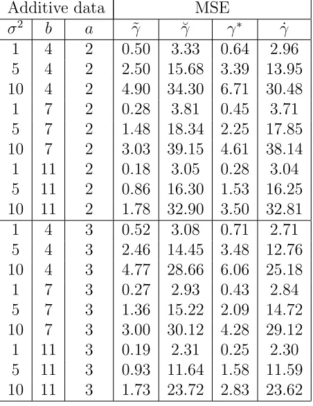
Table 2.8 includes the MSE for each of the point estimators for the additive data. The formula for MSE is M SE = _N1 P

(estimate − parameter value)2_{. Unsurprisingly the}

(61)

Table 2.7: Simulation results for additive data. First three columns describe experi-mental setup. Empirical rejection rates are given for both ACMIF and Tukey’s test for non-additivity at α = 0.05. Results are based on 1,000 MC data sets. The ∗ denotes a run significantly different from actual error rate α= 0.05 (unadjusted p-value=0.00207). Standard error for all proportions presented less than 0.0159.

Additive Data Empirical rejection rates

σ2 _b _a _ACMIF _Tukey

1 4 2 0.046 0.060

5 4 2 0.051 0.041

10 4 2 0.065∗ 0.054

1 7 2 0.037 0.045

5 7 2 0.032 0.056

10 7 2 0.033 0.042

1 11 2 0.037 0.043

5 11 2 0.051 0.034

10 11 2 0.047 0.054

1 4 3 0.052 0.049

5 4 3 0.051 0.048

10 4 3 0.049 0.060

1 7 3 0.030 0.052

5 7 3 0.036 0.051

10 7 3 0.037 0.045

1 11 3 0.041 0.040

5 11 3 0.044 0.057

(62)

Table 2.8: MSE results for four types of estimators for additive data. First three columns describe experimental setup. Other columns report mean squared error for the various estimators. Results are based on 1,000 MC data sets.

Additive data MSE

σ2 _b _a _˜_γ _γ_˘ _γ∗ _γ_˙

(63)

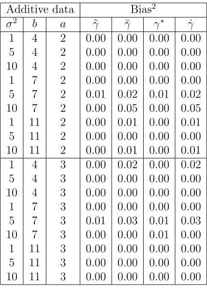
Table 2.9: Squared bias results for four types of estimators for additive data. First three columns describe experimental setup. Other columns report squared bias for the various estimators. Results are based on 1,000 MC data sets.

Additive data Bias2

σ2 _b _a _˜_γ _˘_γ _γ∗ _γ_˙

(64)

Table 2.10: Variance results for four types of estimators for additive data. First three columns describe experimental setup. Other columns report variance for the various estimators. Note variance+Bias2 =M SE. Results are based on 1,000 MC data sets.

Additive data Variance

σ2 _b _a _˜_γ _γ_˘ _γ∗ _γ_˙