NCDOT Technical Report
Identification of Flooded Road Segments Using
LIDAR Elevation Data and 3-D Road Data
By
Hubo Cai
William Rasdorf
Introduction
This section describes the background information for this project, the main goal of this project, and the potential benefits of doing this project.
Background
North Carolina faces extreme hazards and consequences from hurricanes and flooding. Since 1989, there have been 14 federally declared disasters in North Carolina. Damage from Hurricane Floyd alone has reached $3.5 billion. Hurricane Floyd destroyed 4,117 uninsured and under-insured homes. The State’s vulnerability to hurricanes and flooding make it crucial that communities and property owners have accurate, up-to-date information about the flood risk.
Hurricane Floyd revealed flood hazard data and map limitations in North Carolina. Approximately 75% of North Carolina Flood Insurance Rate Maps (FIRMs) are at least 5 years old. Approximately 55% of North Carolina FIRMs are at least 10 years old. Therefore, it is extremely important to obtain up-to-date flood data, which is the major goal of the presently undergoing flood mapping program in North Carolina.
Hurricane Floyd also presented a critical concern to the North Carolina Department of Transportation (NCDOT), i. e., providing information regarding roads under flood to other agencies to determine rescue routes. Obviously this is a very critical task under emergency and rescue scenarios such as hurricanes and flooding. Furthermore, it is different from flood mapping, which aims at predicting flood zones such as 100-year flood zones and 10-year flood zones. The problem facing NCDOT is that how to identify road segments under flood in a real-time way rather than identifying road segments in those flood zones.
Research Needs and Goal
North Carolina is a state that is extremely vulnerable to hurricanes and floods, as state earlier and proved by Hurricane Floyd. Under a flooding scenario, it is critical to determine rescue and response routes so that people and supplies could be distributed promptly and in a timely manner. Unfortunately there is no currently available information system that provides road flood information to rescue activities. It is not unusual for a rescue team to go along a road for a while before they realized that part of that road is under flood and becomes a barrier. This will cause delays in rescue. These delays are very expensive. They cost not only property damages, but also lives. Therefore, it is extremely important to establish such a real-time prediction system.
Since North Carolina is undertaking the flood mapping program using LIDAR technology, it comes naturally the following question: Couldn’t we take the flood maps to predict road segments under flood? This idea was denied for a few reasons as below. First, flood maps categorize areas into 100-year flood zones, 50-year flood zones, 20-year flood zones, and etc. They predict the flood risk for areas rather than anything else. Therefore, it is unsuitable to use flood maps to identify road segments under flood. Second, when a flood occurs, road segments in the flooded area might not be flooded at all or just partially flooded and could be used as the rescue routes.
Significance
This real-time road flood prediction system will provide real-time information regarding road segments under flood when a flood attacks. In addition to identifying and highlighting road segments under flood, it will also provide useful information regarding the depth of water on road segments under flooded so that rescue routes could be determined. By doing this, it will avoid delays in emergency response and rescue, provide information for resource allocation and distribution, and therefore, save time and cost.
Methodology
This section describes the problem of road flood prediction, conceptual model, and computing algorithms.
Water Body
A water body becomes a water body only because part of the area is lower than the surrounding areas as in case of lakes, rivers, and streams. This research project focuses on water bodies including rivers, streams, and lakes. It is obvious that all these water bodies occupies certain areas. In sense of geographical modeling, these water bodies could be modeled as polygons. However, similar to the way that is being used to model roads, rivers and streams could be modeled as linear objects using polylines. In addition, a polygon can be modeled as polylines connected together as illustrated in Figure 1. In case a river is quite wide, which makes it unreasonable to be modeled as a single polyline, two polylines running roughly parallel to each other could be used as illustrated in Figure 1. To summarize, in this study all water bodies are modeled using polylines.
Figure1 Modeling Water Bodies Using Polylines
Conceptual Model
In order to predict road segments under flood, it is necessary to examine the situation in detail. In reality, this problem consists of two parts: first, the water body floods (water level is higher than the normal) and water flows to the surrounding areas; second, the flowing water hits roads and make portions of roads under flooding. The extent to which water flows to the surrounding areas depends on the surface or elevation changes of the surrounding areas. Determining which road segments are under flooding depends on the elevations of the road and the flood level. Figure 2 provides a cross-sectional view of how water body floods and water runs to the surrounding areas. In Figure 2, the blue line represents the normal water level. The red line represents the
River/Stream Modeled
as A Polyline Lake Modeled Using Two Connected Polylines
water level when flooding. It is obvious that there are surrounding areas that were not under water before flooding bur are under water after flooding (areas having elevations higher than the blue line but lower than the red line). The yellow line represents another flood level, in which area A is not flooded even though its elevation is lower than the yellow line, because area B becomes a natural barrier for the water to flood into area A.
Figure 2 Cross-sectional View of Flooding
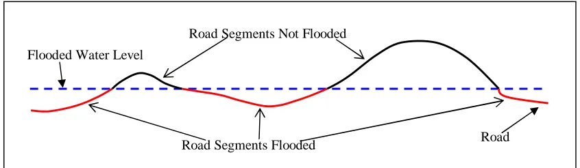
Figure 3 provides a profile of a road segment with several portions under flood. As illustrated in Figure 3, part of the road segments may not be flooded even though its in the flooded area because a road is a three-dimensional object with elevations changing along it.
Figure 3 Illustration of Flooded and Not Flooded Road Segments in the Flooded Area
According to Figures 2 and 3, in order to predict flooded road segments, at least two models will need to be developed. The first one will predict the extent to which water flows when flooding based on the elevations of the surrounding area and the flooded water level. The second will identify flooded road segments for roads running through the flooded areas.
Model 1 ---- Predicting Flood Extent
It was realized that water level (the elevation of the water surface) varies throughout a water body as in the case of river. It is infeasible to assume a uniform water level in a relatively large area. Rather than obtaining water levels at different locations via direct measurements, a surrogate was taken to establish the flood extent prediction model by assuming that at a given point on the a polyline being used to model a water body, the water level equals the elevation of that point. This elevation comes from elevation data such as LIDAR DEMs.
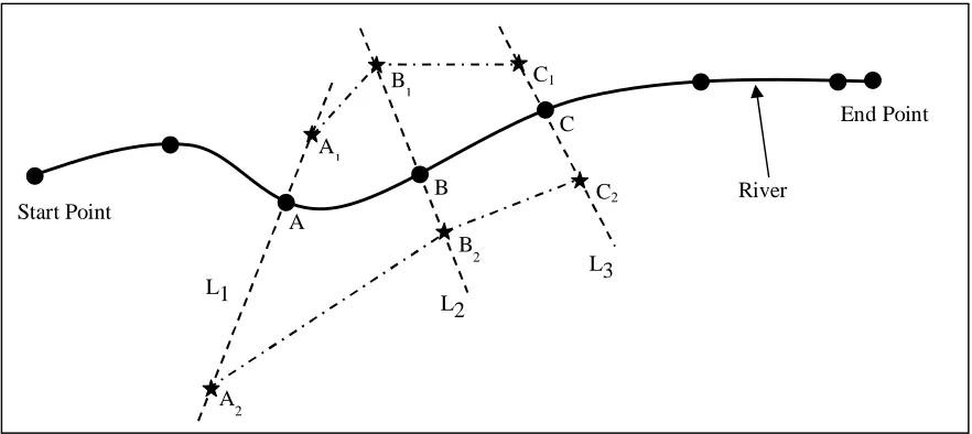
Figure 4 illustrates how the flooded area is predicted when assuming a given flood level (the increase of water level when flooding from the normal water level. In Figure 4, the river is represented with a polyline. A few points that are uniformly distributed along the polyline (with the same interval) starting from the start point of that polyline are obtained. In addition, the start
Normal Water Level Flooded Water Level
Area A Area B
Surface Line
Road Profile Segments Flooded
and end points of that polyline are obtained. At each of these points, a line normal to the river polyline is constructed. For example, at point A, a normal line L1 is constructed. Along this line L1, two points (A1 and A2) are identified. These two points are on two different sides of the river polyline and have elevations equaling the elevation at point A plus the given flood. For example, if point A has an elevation of 105 ft and the given flood level is 2 ft, points A1 and A2 will have the same elevation of 107 ft. After points A1 and A2 are identified, a straight line between these two points is constructed. A set of straight lines will be produced by performing this process with every point and consequently a set of neighboring polygons are constructed by closing lines of neighboring points. For example, two polygons (polygon A1A2B2B1 and polygon B1B2C2C1) can be constructed by closing lines A1A2 with B1B2 and by closing lines B1B2 with C1C2. Each of these polygons will have a water level, which takes the average of elevations at points A and B plus the given flood level.
Figure 4 Conceptual Model for Predicting Flood Extent
According to this flood extent prediction model, the issue of continuously varying water level along a river water body is addressed. In case the water body is a lake that is being described using connected polylines or the water body is still a river but being described using approximately parallel polylines, the polygons surrounding the polylines describing the water body will still be constructed. However, only the parts that are located at the outer direction will be taken. For example, only the polygons A1ABB1 and B1BCC1 will be used, or only the polygons AA2B2B and BB2C2C will be used, depending on the spatial relationship between the polylines being used to describe a water body and the actual location of the water body.
Model 2 ---- Identifying Flooded Road Segments
As stated earlier, even a road segment is within a flooded area, it does not mean that the whole road segment is under flood. In this research project, the flooded area is predicted by using the flood extent prediction model described in the previous section. This flood extent prediction model uses digital elevation data (LIDAR DEMs, more specifically) to determine the flood extent. LIDAR DEMs are in the format of grid files consisting of numerous uniform rectangular cells. Each cell possesses a single value (representative elevation). In the flood extent prediction model, it is this representative elevation that is used to determine if a cell is under flood or not.
However, it is obvious that the elevations of points within a single cell still vary and therefore, for a road segment in the flooded area, it is very possible that only parts of that road segment is flooded as illustrated in Figure 5. It is the main goal of our flooded road segment identification model to identify those parts and differentiate them from the rest of the road segment.
Figure 5 Conceptual Model for Identifying Flooded Road Segments
Computational Model
After the conceptual models are established to describe the problems we are facing, with several assumptions to facilitate problem solving, computational models and algorithms will need to be developed. This section describes the developing environment, data sources, algorithms. Developed codes are attached to this report as appendices.
Developing Environment
The developing environment chosen in this research project is ArcGIS from Environmental Systems and Research Institute (ESRI) and Visual Basic from MicroSoft, which is embedded in ArcGIS. This decision was made based on the source data format, the software availability, and the researchers’ knowledge and skills in programming.
The version being used is ArcGIS 8.3. It consists of ArcMap, ArcCatalog, ArcTools, and etc. ArcMap, ArcCatalog, and ArcTools were used a lot for data management, visual inspection, and analysis. The customized programs were developed using Visual Basic and ArcObjects.
Data Source
Three major data sets were used in this project. They are water body data, LIDAR DEMs, and Road data.
The water body data are in the format of a line shapefile. They are provided by NCDOT. The LIDAR DEMs are downloaded from www.ncfloodmaps.com, which is undertaking the flooding mapping program in North Carolina to obtain elevation data with a high accuracy and consequently, to produce flood maps statewide. The downloaded LIDAR DEMs have a resolution of 20ft. The road data were provided by another closely related research project based on NCDOT LRS data and 3-D LIDAR points downloaded from www.ncfloodmaps.com. The road data are deemed as 3-D data. Each road segment is associated with a set of 3-D points (with X/Y/Z coordinates) along the road segment. For these 3-D points, their X/Y coordinates came from NCDOT LRS road data and their Z coordinates came from 3-D LIDAR points via a snapping approach. The average density of these 3-D points along road segments is
Road Flooded Water Level
Road Segments Not Flooded
approximately 15ft. This snapping approach is not described in this report because it is out of the scope here.
To summarize, the water body data are two-dimensional line data. The road data are three-dimensional data, which are represented as two-three-dimensional line data associated with sets of 3-D points along road segments. The LIDAR DEMs are the elevation data being used to describe the surface.
Preprocessing
Before these data sets could be used to perform analysis, some fundamental preprocessing measures were taken. The LIDAR DEMs were organized as individual grid files. Each of these grid files covers a rectangular area with the size of 10,000ft * 10,000ft. After downloading these individual files, they were merged together to generate a single yet huge file.
The coordinate system being used is the State Plane Coordinate System in feet. The horizontal datum is NAD83. The vertical datum is VNAD83 in feet. All there data sets were reprojected into the same coordinate system.
After preprocessing, these three data sets are ready for the flood extent analysis and flood road segment analysis.
Algorithms
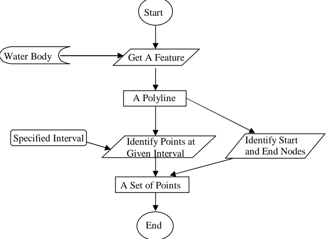
Algorithms were developed respectfully for the two models. Figures 6 and 7 describe the algorithm being used to predict the flood extent with given flood level, water body polyline, and elevation from LIDAR DEMs.
Figure 5 Obtaining Points along A Polyline
Start
Water Body
End Get A Feature
A Polyline
Identify Start and End Nodes
In Figure 5, from the water body data (a line shapefile), a feature is obtained. This feature is a polyline. By identifying the start and end nodes of this polyline and identifying points along the polyline, which are uniformly distributed at the specified interval from the start point, a set of points are obtained for a polyline. Repeating this procedure for all features in the water body data results in sets of points. Each set of these points is associated with one polyline feature describing the water body. These points are distributed along the polyline features uniformly at the specified interval.
Figure 7 The Procedure of Predicting Flood Extent
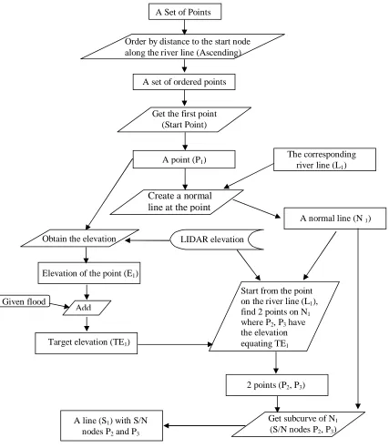
Figure 7 describes the procedure of constructing normal lines to the water body polyline at those points identified in Figure 6. First, a set of points is taken and ordered in ascending according to
A Set of Points
Create a normal line at the point
A line (S1) with S/N
nodes P2 and P3
The corresponding river line (L1)
A point (P1)
Get the first point (Start Point) A set of ordered points Order by distance to the start node along the river line (Ascending)
Obtain the elevation
A normal line (N 1)
Get subcurve of N1
(S/N nodes P2, P3)
2 points (P2, P3)
Start from the point on the river line (L1),
find 2 points on N1
where P2, P3 have
the elevation equating TE1
LIDAR elevation
Target elevation (TE1)
Add
Elevation of the point (E1)
their distances to the start node of the corresponding polyline. For each of these points, a line normal to the polyline is constructed based on the curvature of the polyline. The elevation at such a point is determined based on the LIDAR DEMs. Adding together this elevation with the given flood level leads to the target elevation. Two points having the target elevation on the normal line are identified. For example, assuming the original point is point A with elevation E1, two new points A1 and A2 will be identified on the normal line. Both of these two points have the target elevation, which equals the sum of the elevation at point A and the given food level. Furthermore, there will be no points between A and A1 and between A and A2 along the normal line, which have elevations higher than the target elevation. In other words, A1 should be the first point that reaches the target elevation starting from A in one direction. Similarly, A2 should be the first point that reaches the target elevation starting from A in another direction. After A1 and A2 are identified, a straight line connecting A1 and A2 can be constructed and later on, this line will be used together with another such lines being constructed at the neighboring points of point A to construct polygons that represent the flood extent.
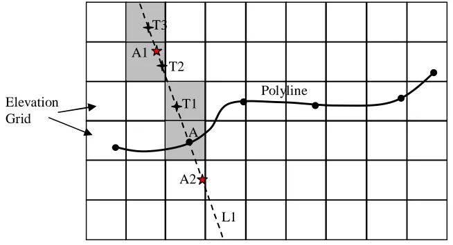
The critical part of this procedure is how the two points A1 and A2 are identified based on the elevation data. Figure 8 illustrates this identification procedure in detail. In Figure 8, line L1 is the normal line constructed at point A. Point A1 is the point that has the target elevation and is the point need to be identified. The procedure is described as below:
1) The elevation of the cell in which point A is located is obtained.
2) Elevation at point A is added with given flood level to obtain the target elevation.
3) Starting from point A along the normal line, point T1 is identified. The distance between A and T1 equals the resolution of the elevation grid file (the height or width of a cell).
4) The elevation of the cell containing point T1 is obtained and compared to the target elevation. If this elevation is lower than the target elevation, another point T2 along the normal line is obtained. The distance between T2 and T1 equals the resolution of the elevation grid file. The elevation of T2 is compared to the target elevation. This step is repeated until the first point having elevation higher than the target elevation is obtained.
5) Assuming the first point having elevation higher than the target elevation is T3, it indicates that point T2 has an elevation lower than the target elevation. Taking a linear interpolation approach to identify a point A1 between T3 and T2 on the normal line, which has its elevation equaling to the target elevation. This point A1 is the point need to be identified. 6) Repeat steps 3) to 5) to identify point A2 on the other side.
Figure 8 Identifying Points with Target Elevation
Using these algorithms, the flood extent is predicted. The predicted flood extent consists of numerous polygons. Each of these polygons has a flood level. This set of data will be used later to identify road segments under flood. The program developed for flood extent prediction using Visual Basic and ArcObjects is attached as Appendix A.
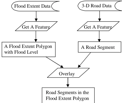
Figures 9 and 10 illustrate the algorithm of identifying portions of a road segment that are under flood when that road segment runs through the flooded area. This algorithm uses two data set: the flood extent data obtained from the flood extent prediction algorithm and the 3-D road data obtained from another research project as stated earlier.
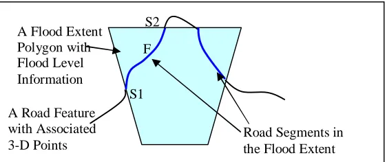
Figure 9 illustrates the first part of the algorithm. Each feature (a polyline) in the 3-D road data is overlaid with each feature (a polygon) in the flood extent data. By doing this, road segments in the flood extent are all identified. In addition, since this procedure is repeated with a single feature from the 3-D road data and a single feature from the flood extent data, the corresponding 3-D road features and flood levels are also identified and associated with the identified road segments. More specifically, each of the road segments identified as in the flood extent has the information in the following format: road segment A corresponds to road feature with ID F, starts from S1, and ends at S2; the corresponding water flood level is E. This is illustrated in Figure 11. Points S1 and S2 are located via their distances to the start point of the road feature on which they are located.
Figure 9 Flood Road Segment Identification Algorithm, Part I
For each of the road segments identified in Part I of the algorithm, Part II is performed as illustrated in Figure 10. First, a set of 3-D points between the start and end points of the segment are obtained from the 3-D road data. In addition, the start and end points of the identified road segment are obtained and their elevations linearly interpolated from the 3-D road data. With a set of 3-D points covering the complete road segment, all portions of this road segment that are under flood are identified (refer to Figure 5 for concepts). This is the critical part of the algorithm and it is illustrated in Figure 12.
Flood Extent Data 3-D Road Data
Get A Feature Get A Feature
A Flood Extent Polygon with Flood Level
A Road Segment
Overlay
Figure 10 Flood Road Segment Identification Algorithm, Part II
Road Segments
Identified in Part I Get One Segment
A Road Segment 3-D Road Data
Obtain All 3-D Points between the Start and End Points and Obtain Elevations for the Start and End Points via Linear Interpolation
A Set of 3-D Points Covering the Complete Road Segment
Sort Ascending, Based on Their Distances to the Start Point
A Sorted Set of 3-D Points Covering the Complete Road Segment
Identify the First 3-D Point Having Elevation <= Flood Level
Exists? Yes No
Identify the First 3-D Point P1 Having Elevation = Flood Level Stop
Point P1
Identify the First 3-D Point Having Elevation >= Flood Level (starting from P1)
Exists? Yes No
Identify the First 3-D Point P2 Having Elevation = Flood Level (starting from P1)
P2 = S2
Point P2 Subcurve from
P1 to P2
P2=S2? Yes
No
Stop Start from P2
Is it S1? Yes
No
Figure 11 Identifying Road Segments in the Flood Extent
In Figure 12, the black dots represent all 3-D points on the road segment. Except the start and end points, all these 3-D points come directly from the 3-D road data. For the start and end points, their elevations are obtained by linearly interpolation. For example, for the start point, its elevation is linearly interpolated from two neighboring 3-D points in the 3-D road data. One 3-D points is right before the start point and the other is right after the start point based on their distances to the start point of the corresponding 3-D road feature.
The essence of identifying flooded road segments is to identify those points with elevations equaling the flooded water level, which are represented with light blue stars. According to the algorithm described earlier, the first point with elevation less than or equal to the flooded water level is S1 and therefore, S1 is assigned to point P1. Starting from P1, the first point with elevation greater than or equal to the flooded water level is point T1. A linear interpolation will be used on point T1 and point T2, which is the 3-D point right before T1. By doing this, point P2 is located. Its elevation equals to the flooded water level. After identifying points P1 and P2 a sub-curve of the road segment starting from P1 and ending at P2 is generated. This sub-curve is under flood.
According to the algorithm illustrated in Figure 10, since P2 is not S2, this procedure will continue starting from point P2. Consequently, points T3 and T5 will be found, new P1 and P2 are obtained, and a new sub-curve will be obtained. Repeating this procedure will identify all flooded portions of that road segment.
Figure 12 An Illustration of Identifying Flooded Road Segment Algorithm
A Flood Extent Polygon with Flood Level Information A Road Feature with Associated
3-D Points Road Segments in the Flood Extent S1
S2 F
Road Segment Flooded Water Level Road Segments Not Flooded
Road Segments Flooded Road Segment outside
Flood Extent
Road Segment outside Flood Extent
S1 S2
T1 T2 P2
T3
T4 T5
Again, a program developed in Visual Basic using ArcObjects is attached to this report as Appendix B.
Variants
There are a couple of variants to the models and algorithms, which have been under consideration. Two of these variants are described hereby for future considerations. One of them is for predicting flood extent. The other is for identifying flooded road segments.
As described earlier, the flood extent prediction model in this research project takes such an approach that at every point (points uniformly distributed with a given interval) a normal line is constructed. On this normal line, two points having the target elevation (flood water level) are identified and a straight connecting these two points is generated. This line will be connected to such lines generated from the neighboring points to construct flood extent polygons.
The flood extent prediction variant differs from the model described earlier. While points uniformly distributed will still be identified, normal lines will not be constructed. Rather, the variant works with the grid cells in a more direct way. For each of those point identified, a cell is identified, which contains that point. The target elevation is still the elevation value of that cell plus the given flood level. The neighboring cells (totally 8 cells) of that cell are examined. If a cell has its elevation lower than the target elevation, this cell is identified as in flooded area and is assigned with the target elevation to indicate flooded water level. This procedure is repeated until no such cell is found in a cycle, which indicates the flood extent due to this specific point along the water body polyline is complete.
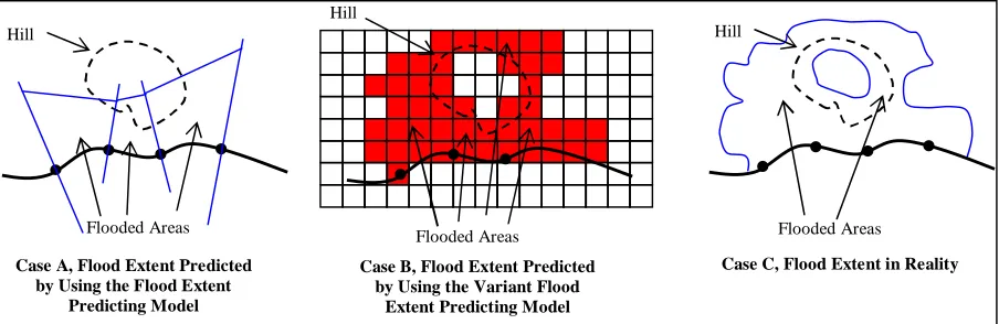
The advantage of this variant is its strength in solving a scenario as illustrated in Figure 13 because this variant simulates the actual situation of flooding in a more real way than the flood extent prediction model described before. In Figure 13, there is a hill right besides the water body. Case C shows that in reality, the flooded area (the ring constructed by two blue lines and the water body polyline) includes the area behind the hill. In Case A, which illustrates the flood extent predicted using the flood extent prediction model, the flooded area behind the hill is not included in the predicted flood extent. However, if the variant is taken as illustrated in Case B, the flooded area behind the hill is included as indicated by the red cells. In other words, in a scenario as illustrated in Figure 13, the variant might be more realistic. The disadvantage of this variant is its complexity and consequently, its difficulty of being developed.
Figure 13 The Difference between the Flood Extent Prediction Model and Its Variant in Dealing with One Particular Scenario
Hill Flooded Areas Hill Flooded Areas Hill Flooded Areas
Case A, Flood Extent Predicted by Using the Flood Extent
Predicting Model
Case B, Flood Extent Predicted by Using the Variant Flood
Extent Predicting Model
In case of the variant for identifying flooded road segments, it differs from the model described earlier in its assumption. More specifically, the variant simply assumes all road segments in the flooded areas are flooded. In other words, with this assumption, those small polygons representing flood extent can be simply merged together to construct bigger polygons to represent flood extent without keeping flooded water level for each of those small polygons. All road segments in the bigger flood extent polygons are identified as road segments under flood without considering the third dimension of roads (the elevation). The advantage of this variant is its simplicity. The disadvantage of this variant is its incapability of identifying road segments that are in the flooded areas but not flooded, which occurs frequently in the reality.
Testing
This section describes the results of testing the flood extent prediction model, the model for identifying road segments under flood, and their corresponding algorithms. In addition, the second variant (the variant which simplifies the approach of identifying road segments under flood) is tested.
Study Area
The study area for testing the models and algorithms is chosen to be part of the Wilson County in North Carolina. There are a few of reasons of choosing the study area as illustrated in Figure 14. First, according to the conversation with NCDOT personnel, there are high-quality water body data in this area. Second, LIDAR data are available in this area. Third, 3-D road data are available in this area. Forth, there are roads that are close to the water body and therefore, will produce meaningful results.
In Figure 14, the read lines (“Dis_int_wilson”) represent the Interstate highways in Wilson County. The “river_feet” represents all water bodies in Wilson County. The blue lines (“Testing_riv_3”) represent portions of the water bodies that are under testing. Please note while only portions of roads and water bodies in Wilson County are included in the testing scope, the LIDAR elevation data are countywide, or they cover the complete county of Wilson.
Results
This subsection describes the results of testing our models and algorithms in the study area.
Flood Extent Prediction
The flood extent prediction model and its associated algorithm are tested with the water body data in the study scope with different combinations of flood levels and intervals.
1) 2ft Flood Level, 100ft Interval
Figure 15 shows the testing result of predicting the flood extent with a flood level of 2ft while taking points every 100ft along the water body polyline. In Figure 15, the blue lines represent water body polylines in our study area. The green polygons represent areas that are predicted as the flood extent.
Figure 15 Testing Result of the Flood Extent Prediction Model (100ft Interval, 2ft Flood Level)
not easy to see the small polygons. They will be illustrated later in detailed pictures. The problem of those big polygons will also be addressed later in the Observations of Flood Extent Prediction subsection with explanations and countermeasures.
2) 2ft Flood Level, 200ft Interval
Figure 16 shows the testing result with the same flood level (2ft), but a bigger interval (200ft).
Figure 16 Testing Result of the Flood Extent Prediction Model (200ft Interval, 2ft Flood Level)
3) 2ft Flood Level, 500ft Interval
Figure 17 shows the testing result with the same flood level (2ft), but the biggest interval (500ft).
4) 4ft Flood Level, 500ft Interval
Figure 18 shows the testing result with a flood level of 4ft and an interval of 500ft.
Figure 18 Testing Result of the Flood Extent Prediction Model (500ft Interval, 4ft Flood Level)
5) 4ft Flood Level, 200ft Interval
Figure 19 shows the testing result with a flood level of 4ft and an interval of 200ft.
In addition to the results shown before, Figures 20 and 21 illustrate some small polygons surrounding the water body polylines, i.e. the first group of polygons that indicate the flood extent.
Figure 20 Detailed View 1
Observations of Flood Extent Prediction
The testing results show that the predicted flood extent consists of numerous polygons with different sizes and flood water level. As state before, these polygons can be categorized into two groups: small polygons surrounding water body polylines in a neat way and big polygons reaching the boundary of the elevation data being used to predict the flood extent.
The existence of those big polygons reveals that there is a problem with the flood prediction model. As stated earlier, polylines are used to describe water bodies and the water levels along these polylines are assumed to be the same as the elevations along these polylines, which come from the elevation data set. While LIDAR is capable of providing high-accuracy elevation data, its capability is limited to areas surrounding water bodies because water absorbs most of the source pulses and only a very little portion of the source pulses are reflected and therefore, affects the accuracy of LIDAR elevation data surrounding water bodies. In addition, the LIDAR elevation data used in this project are bare earth data in the grid format, which consists of rectangular cells. Each cell is the size of 20ft * 20ft, but has the average elevation of LIDAR points in the cell as the representative elevation. In addition, the positional accuracy of the water body polylines is questionable. Describing a narrow water body with a single polyline or the positional error of polylines describing the edges of a relatively wide water body lead to the use of incorrect elevation values.
A typical situation (cross-sectional view) is illustrated in Figure 22. In Figure 22, the blue line represents the normal water line. The red line represents the water level when flooding. However, with the water body data being used, a single line is being used to describe the water body at the position indicated by the black point. Consequently, incorrect elevations are used and a false flood water level is generated (green line). According to Figure 22, the top of the left hill surrounding the water body is missed. In other words, even there is a point (the hilltop) that is higher than the flood water level, it is not captured when applying our flood extent prediction. As a result, the constructed polygon will reach the boundary of the elevation data set (the algorithm works in such a way that if there is no point having elevation higher than the flood water level, then the boundary of the elevation data is taken to define the flood extent). This is the reason that there are a few big polygons reaching the boundary of our elevation data (in our case, the county boundary).
Figure 22 Illustration of False Flood Water Level and Resulting Big Polygons
This problem could be solved by identifying these big polygons that reach the county boundary and delete them in the way illustrated in Figure 23. In Figure 23, polygon P1 reaches the boundary is a big polygon (point F and G reache the boundary). This polygon is identified and
Earth Surface
Normal Water Level Flood Water Level
False Position of the Polyline Representing Water Body
deleted together with its two neighboring polygons (P3 and P4). Only points not reaching the boundary are used to construct polygons P2, P5, and P6 instead.
Figure 23 A Proposed Approach to Deal with the Problem of Polygons Reaching Boundary
In addition to the problems associated with big polygons reaching boundary, there are a few of important observations regarding the variations of interval and flood level. They are listed as below.
• Smaller interval results in more number of polygons. • Bigger flood level results in larger predicted flood extent.
• Smaller interval increases the significance of those big polygons reaching the boundary. • The majority of the resulting polygons from two different intervals overlap a lot.
• With the same flood level, the resulting polygons from a bigger interval do not cover the resulting polygons from a smaller interval. Neither do the resulting polygons from a smaller interval cover the resulting polygons from a bigger interval.
To summarize, the flood extent prediction model of this research project is technically feasible with reasonable results. Different combinations of flood levels and intervals lead to different results. However, there is no definite answer to the question regarding the optimum combination of flood levels and intervals that should be used to obtain accurate results.
Flooded Road Segment Identification
After the flood extent is determined with given flood level and interval, the second model and its associated algorithm (the flooded road segment identification model) can be applied to obtain determine flooded road segments. In applying this model and its algorithm, the 3-D road data mentioned earlier play a critical role.
Figure 24 shows the results of applying this model when using the results of the flood extent model with the flood level of 4ft and the interval of 500ft. In Figure 24 the identified flooded road segments are highlighted.
After Before
P1 A
B C
D
A
B C
Figure 24 Identified Flooded Road Segments
Figure 25 provides a detailed view of the identified flooded road segments. It is obvious that for a road segment within the flood extent it does not mean that this road segment is completely flooded. Table 1 provides part of the attribute table, which contains helpful information to identify the flooded road segments easily. The column with the heading of “MERGE” identifies the road feature in the 3-D road data, of which the flooded road segments come. The columns with headings of “Start” and “End” specifies the planimetric distances from the start and end points of the flooded road segment to the start of that particular road feature. Consequently, with
Legend
Interstate Highway Flooded Road Segment
this information, the flooded road segments can be easily identified in addition to the visual result as shown in Figure 24 and therefore, can be combined with other data for further analyses.
Figure 25 Detailed View of the Identified Flooded Road Segments Legend
Interstate Highway Flooded Road Segment
Table 1 Part of the Attribute Table of the Identified Flooded Road Segments FID Shape MERGE Start End
0 Polyline 1 16268.6676 16727.8315
1 Polyline 1 25156.4506 25380.1103
2 Polyline 1 28723.0097 29402.4092
3 Polyline 1 27629.4739 28723.0097
4 Polyline 2 16993.5179 17597.3257
5 Polyline 2 17597.3257 18524.5620
6 Polyline 2 11142.0085 11908.6555
7 Polyline 2 21084.6812 21183.0234
8 Polyline 2 10422.6277 10742.9855
9 Polyline 2 9247.3923 9790.3087
10 Polyline 2 7324.4328 7902.3860
11 Polyline 2 6434.6108 7324.4328
Results of an Variant in Identifying Flooded Road Segments
Figure 26 Identified Flooded Road Segments Using the Simplified Variant Legend
Interstate Highway
Figure 27 Detailed View of the Identified Flooded Road Segments Using the Simplified Variant
One more thing could have been done is to merge the polygons together. In case the simplified variant is used, it is unnecessary to keep those small polygons as individual ones (the only reason of keeping them as individual ones is that each polygon is associated with a flood level, which will in turn to be used to identify flooded road segments). With the simplified variant, this flood level information will not be used because it assumes all road segments in the flood extent are flooded. Since this can be easily done with GIS (for example, the “Dissolve features based on an
Legend
Interstate Highway Flooded Road Segment
attribute” option under the GeoProcessing Wizard can merge polygons together based on an attribute such as the river ID), the result of this merge process is not shown here. However, the author has tested this procedure and was successful.
Problems Identified
By carrying out the testing for our models and associated algorithms, a few problems/shortcomings were identified. These problems/shortcomings will be discussed in detail in this section.
The first problem identified is the problem of those big polygons reaching the boundary of the elevation data. As described earlier, this problem is the result of two issues. First, the water level at a specific point of a water body polyline is assumed to be the same as the elevation at that point. Second, with this assumption, a small positional error might lead to the missing of a hill-top with a relatively high elevation and consequently, the flood extent being predicted will reach the boundary to generate the big polygons. This issue could be addressed using the procedure described in Figure 23.
Furthermore, it was considered that the water monitoring sites could be used to provide water level at those sites and the water levels at any other locations could be interpolated. However, examining the locations of all water monitoring sites in North Carolina revealed that the density of these water monitoring sites is far from satisfactory. For example, with the water monitoring location data NCDOT has, there is only one such site in Wilson County and consequently, it is impossible to be used to estimate water levels. Another thought is to take the bridge data being maintained by NCDOT. The bridge data contain information regarding the 3D locations of bridges and their heights above water. Taking into consideration of the density of bridges in North Carolina, this will provide reasonable interpolations. However, there are still some problems with this surrogate. First, for an individual water body, there is no guarantee that there will be enough number of bridges above it. Second, there is still no guarantee that the heights above water were obtained at normal water levels. Regardless of these problems, it remains to be a possible surrogate and will need further research.
The second problem is the problem of using polylines to describe water bodies. With a relatively narrow water body, a polyline will be used. With a relatively wide water body, polylines will be used to locate the edges of that water body. However, the water levels are always changing and therefore, the location of water body edges is always changing. In other words, those edges should be determined under a condition named “normal water level”, which is hard to do and is almost infeasible for a statewide study scope.
The third problem is related to the flood extent prediction model in dealing with the scenario as illustrated in Figure 13. As stated earlier, this problem could be solved by taking the variant approach rather than the flood extent prediction being used.
There is also a potential problem associated with using the 3-D road data. All 3-D points along roads are not uniformly distributed and therefore, when using the linear interpolation to determine a point elevation might be questionable at a place where the distance between two neighboring 3-D points are far from the average density (approximately 15ft).
Further Improvements
Further improvements to flood extent prediction could be taken when taking into consideration of the geometric characteristics of water bodies. First, the elevation at a point along the centerline of a water body should be lower than or equal to all its surrounding points. Second, water runs in one direction. In other words, if points A, B, C, and D are four points along the centerline of a water body and water runs from A to B, C, and D, the correct descending order of water levels at these 4 points should be A – B -- C – D.
Based on these two characteristics, two improving measures are taken to make sure points taken along the centerline of water bodies meet the two criteria described earlier. In order to obtain sufficient points for polygon construction, this time the interval is specified to be the resolution of the LIDAR DEM data (20ft). With each of these points, it is checked according to Figure 28. First, the cell of the elevation data, which contains the given point (in this case, cell 0) is identified. Next, all its neighboring cells (cells from 1 to 8) are identified. The elevation value of cell 0 is compared to elevation values of cells 1 to 8. If the elevation value of cell 0 is the smallest (the lowest elevation), this point is kept for polygon construction. Otherwise, it’s discarded.
Figure 28 Checking Elevations with Surrounding Cells
Figure 29 shows the testing results by applying the first improving measure as described earlier. In this case, the interval is no longer uniform. The flood level is 2ft. In addition, the procedure illustrated in Figure 23 is taken to deal with the problem of big polygons reaching county boundaries. The code that fulfills checking elevations with surrounding cells is attached in Appendix D. It first takes a uniform interval of 20 ft to obtain points along the centerline of water bodies. All these points are inserted into a blank table. At the same time, these points are checked according to Figure 28 with their surrounding cells. If a point has the lowest elevation among all surrounding cells, this point will be used later in polygon construction and is inserted into another blank table. It is worth pointing out that the procedure of constructing polygons is the same. The only different is that a different set of points along the centerline of water bodies is being used.
1 2 3
4 5
6 7 8
Figure 29 Testing Results of Flood Extent after Checking with Surrounding Cells
The second improving measure is to enforce the business rule regarding how water flows. Figure 30 illustrates this situation. If water runs from point A1 to point A9, then the water levels of points A1 to A9 should appear as scenario 1. If water runs from point A9 to point A1, then the water levels of points A1 to A9 should appear as scenario 2.
Figure 30 Illustration of Water Flow
Examining the points along the centerline after applying the first improving measure revealed that it is not always the case that these points would follow the water flow rule. One example is
A1 A2 A3 A4 A5
A6
A7 A8 A9
A1
Water Level
Water Level
Planimetric View
Vertical Profile – Scenario 1
provided in Figure 31, in which these points are plotted according to their elevations (vertical axis) and their distances to the start point of the centerline (horizontal axis).
Figure 31 An Example of the Vertical Profile of Points along the Centerline
In order to ensure that water is always running downward, the second improving measure is taken. This measure is associated with two different algorithms. Both of them need two constants, an error tolerance (in the units of ft/ft) and a maximum drop (in the units of ft/ft).
Figure 32 illustrates the concepts of error tolerance and maximum drop. In Figure 32, a straight line is used to represent the vertical profile of water. The horizontal axis represents the planimetric distance to the start point. The vertical axis represents the water level. It assumes that water runs from the start point S to the end point E. Points P1 and P2 are two neighboring points that are used to illustrate two scenarios of errors. Ideally, all these points are on the straight line representing the vertical water profile. Scenario A illustrates that point P2 is higher than point P1. Scenario B illustrates that point P2 is lower than point P1. In case of scenario A, the error tolerance is applied. Assuming the planimetric distance from point P1 to S is D1, the planimetric distance from point P2 to S is D2, point P1 has a water level of W1, point P2 has a water level of W2, W2 is higher than W1, and an error tolerance of E1, if W2 <= (W1 + E1 * (D2 – D1)), it is within the given error tolerance and is deemed to be acceptable. On the other hand, if W2 > (W1 + E1 * (D2 – D1)), it exceeds the error tolerance and countermeasures will be taken as described later. In case of scenario B, the maximum drop from point P1 to point P2 is checked. If (W1 – W2)/(D2 – D1) <= Maximum Drop (MD), it is acceptable. Otherwise, it is deemed that the maximum drop is exceeded and countermeasures will have to be taken as described later.
Two different algorithms are taken to deal with neighboring points either exceed the given error tolerance or the maximum drop.
Vertical Profile of Points along the Centerline of A Water Body
0.0000 1000.0000 2000.0000 3000.0000 4000.0000 5000.0000
0.0000 1000.0000 2000.0000 3000.0000 4000.0000 5000.0000 6000.0000 7000.0000
D_TO_S
1) Algorithm 1
In case the error tolerance is exceeded, algorithm 1 assigns the water level of P1 to point P2. In case the maximum drop is exceeded, algorithm 1 assigns point P2 with a water level that is equivalent to (water level of point P1 – Maximum Drop * (D2 – D1)). The code for fulfilling algorithm 1 is attached as Appendix E.
2) Algorithm 2
In case the error tolerance is exceeded, algorithm 2 assigns the water level of P1 to point P2, which is the same as algorithm 1. In case the maximum drop is exceeded, algorithm 1 assigns point P1 with a water level that is equivalent to (water level of point P2 + Maximum Drop * (D2 – D1)), which is different from algorithm 1. The code for fulfilling algorithm 2 is attached as Appendix F.
Figure 32 Error Tolerance and Maximum Drop
Figures 33 and 34 shows the testing results of flood extent prediction after taking algorithm 1 and algorithm 2, respectively, with an error tolerance of 1ft/10ft and the maximum drop of 1ft/50ft.
Figure 33 Testing Results after Applying Algorithm 1
S S
E E
P1 P2 P1
P2 Water
Level
Water Level
Distance from S
Distance from S Scenario A,
Error Tolerance
Figure 34 Testing Results after Applying Algorithm 2
Summary and Conclusions
This research project aimed at identifying flooded road segments in case a flood occurs by using elevation data, water body data, and 3-D road data. With the scenario of flooding clearly described, two models and associated algorithms and program codes were developed. The first model predicts the flood extent and the second model identifies flooded road segments. In addition, variants to these models were discussed.
The developed models and algorithms were tested. The study scope for the testing was limited to part of the Wilson County in North Carolina. Testing results with different parameters (flood level and interval) were presented and examined in detail. In addition, potential problems were identified and countermeasures were proposed and discussed.
It is concluded that the developed models and algorithms worked well in the testing. Even though they still have some potential problems and some further improvements could be done, they provide reasonable results. It is technically feasible to identify flooded road segments with the existing LIDAR elevation data, the water body data, and the 3-D road data generated from another related research project. It is feasible to apply two constants (error tolerance and maximum drop) to ensure that water always runs in one direction (from higher water level points to lower water level points).