Mathematical Models of Dividing Cell Populations: Application to
CFSE Data
H.T. Banks
†and W. Clayton Thompson
†∗†
Center for Research in Scientific Computation
Center for Quantitative Sciences in Biomedicine
N.C. State University
Raleigh, NC
and
∗
ICREA Infection Biology Lab
Department of Experimental and Health Sciences
Universitat Pompeu Fabra
Barcelona
July 30, 2012
Abstract
Flow cytometric analysis using intracellular dyes such as CFSE is a powerful experimental tool which can be used in conjunction with mathematical modeling to quantify the dynamic behavior of a population of lymphocytes. In this survey we begin by providing an overview of the mathematically relevant aspects of the data collection procedure. We then present an overview of the large body of mathematical models, along with their assumptions and uses, which have been proposed to describe the dynamics of proliferating cell populations. While much of this body of work has been aimed at modeling the generation structure (cells per generation) of the proliferating population, several recent models have considered the more fundamental task of modeling CFSE histogram data directly. Such models are analyzed and recent results are discussed. Finally, directions for future research are suggested.
1
Overview
The human immune response is characterized by a large number of complex, interrelated steps in which the body recognizes an invading pathogen and (hopefully) neutralizes the threat posed by that pathogen. In the face of such complexity, quantitative modeling can play an active role in describing and organizing the vast array of biophysical processes underlying the cellular and subcellular mechanisms of the immune response. This information, in turn, has obvious implications for human health in areas such as allergen treatments, immunosuppression for tissue transplants, immunizations, pathogenesis, etc.
The mathematical analysis of lymphocyte activation and division can be performed on scales ranging from the molecular to the population level, and the behavior of individual cells can be highly variable, given the seemingly random intracellular and environmental factors to which a single cell might respond. However, the immune response as a whole (to be understood as the aggregate behavior of all cells in the population) is regular and predictable [77]. In a typical immune response, a small number of cells recognizes and responds to foreign antigen. These initial responders then rapidly produce identical copies of themselves by mitosis and begin to develop effector function in a process known as ‘clonal expansion’ [64, Sec. 1.17]. This clonal expansion–in particular, the rates at which cells activate, divide, and die immediately following antigen recognition–is a key component in characterizing the efficacy of an immune response. Thus, in this review, focus is placed on the processes of cell division responsible for the clonal expansion of lymphocytes following antigen presentation. In particular, a number of mathematical models are surveyed which attempt to describe the numbers of cells (starting from an initially ‘undivided’ population) which have divided a given number of times. They key idea is to link these cell numbers (in terms of the number of divisions undergone) back to the dynamic behavior of dividing cells in order to describe the ‘cellular calculus’ [43] by which cells receive and respond to environmental stimuli.
The mathematical modeling of cell division has long been of interest (see, e.g., [28, 76]) but the many mathematical models proposed over the past 40 years have been hard to validate because of the difficulty of obtaining appropriate experimental data. Unlike many cell types, lymphocytes are inherently mobile. In the context of in vitro studies, the nonadherence of lymphocytes makes it difficult to determine the lineage of cells on a large scale [58]. While video microscopy techniques can be used for such a determination and significant information can be obtained from such studies (see, e.g., [49]) the number of cells which can be effectively monitored is comparatively small. Instead, flow cytometric analysis of a population of cells can be used to assess tens of thousands of individual cells (from a population of millions) accurately and efficiently. Thus one trades information on cell lineage for information from a larger population of cells. While cells are measured individually, individual cells (or their progeny) are not followed over the course of the experiment so that the measurement process is in effect an aggregate sampling. That is, one must useaggregate (or population level) data in an attempt to describe what are ultimately the dynamics of individual cells. This type of inverse problem is well known in mathematics, and successful mathematical models have been developed and fit to data in a variety of applications such as size-structured marine and insect population models [4, 7, 11, 12], wave propagation models for viscoelastic solids [19], electromagnetic wave propagation [13, 14], physiologically-based pharmacokinetics models [6, 20], and HIV models [5]. In addition to these applications, theory for such inverse problems is well-developed [3, 6, 18]. In effect, the mathematical task is to model the processes involved in cell division with limited or no knowledge of familial relation between cells.
Intuitively, one cannot adequately model and estimate rates of cell division and death from knowledge only of the total number of cells in the population at a series of measurement times. For instance, even if one knows that the total number of cells in a population is unchanged between two measurement times, one still cannot say whether the cells are not dividing or are dividing and dying in such a way that the population size is unchanged. Instead, information is needed regarding the generational distribution of cells in the population (that is, the numbers of cells having not yet divided, divided once, twice, etc.). To this end, the relatively recent development of carboxyfluorescein succinimidyl ester (CFSE) by Lyons and Parish [60] as a division-tracking intracellular dye, in conjunction with flow cytometry, has made it possible to quickly and accurately assess generational structure within a population of cells. This is a powerful experimental tool which can be used to augment the formation, analysis, and validation of mathematical models of cell division. These models can then be used for the meaningful quantitative comparison of data sets in different experimental and biological conditions.
number of mathematical models of cell division have been proposed and tested against CFSE-based flow cytometry data. (While CFSE-based data remains the gold standard for model validation, competitive dyes are currently being developed and tested [70].) We begin this report with an overview of the experimental procedure for CFSE-based flow cytometric analysis of a lymphocyte culture, focusing on mathematically relevant aspects of the resulting data (Section 2). Then several mathematical models of dividing cell populations are surveyed (Section 3) and their salient features highlighted. (Readers who find our overview of interest should find the recent manuscript by Miao, et al., [63] also of interest. In this presentation they provide a comparison of four of the type of models considered here: a branching process, the cyton, a Smith-Martin and linear birth-death ODE model, using simulated data. The branching process model, which outperforms the other three, is also applied to CFSE labeled data for CD4+ and CD8+ T cells proliferating after stimulation.) Our report is limited strictly to mathematical models for a dividing population of cells of a single type. In general, the cell dynamics models considered are phenomenological in nature, describing the dynamic behavior of a population of cells without regard for the underlying molecular pathways governing cell behavior. However, the work surveyed here represents an important initial step toward a more complete description of an immune response, and it seems certain that the framework(s) presented here can be generalized mathematically and experimentally to incorporate more complex information.
2
Flow Cytometry and CFSE Data
CFSE can be used on a wide variety of human and murine cell types, including T lymphocytes, B lymphocytes, NK cells, fibroblasts, hematopoietic stem cells, and smooth muscle cells, as well as bacteria [58, 67, 71, 81]. Such CFSE-labeled cells are analyzed by flow cytometry using a standard fluorescein setup [67, 71]. While CFSE can be used both in vitro and in vivo (for animal studies), the models presented in Section 3 are limited to in vitro studies so that the total number of labeled cells can be assessed. An experiment begins with peripheral blood mononuclear cells (PBMCs) which are isolated either from whole blood or a buffy coat. CFSE is introduced into the culture of PBMCs as carboxyfluorescein diacetate succinimidyl ester (CFDA-SE) which is membrane permeable and thus freely diffuses into the cell. Once inside the cell, intracellular esterases remove the acetate groups, producing CFSE which is membrane impermeable and thus bound inside the cell [67, 71]. After the initial CFSE uptake, excess CFSE (or CFDA-SE) is removed from the culture. Inside the cell, further reactions with amino groups result in the rapid degradation or expulsion of some carboxyfluorescein conjugates, while a fraction of the carboxyfluorescein binds to stable intracellular proteins and remains within the cell for an extended period of time [67].
Carboxyfluorescein groups within the cell absorb light from an excitation laser and then release that energy with a peak emission wavelength of 517nm (green). Cells are passed through the flow cytometer one at a time via hydrodynamic focusing and the fluorescence intensity (FI) of the emission from each cell is quantified. It is known that FI varies directly with the mass of CFSE within a cell [58] so that measured FI is a useful surrogate for the mass of CFSE passing through the measurement apparatus. Because cells become fluorescently labeled via the free diffusion of CFDA-SE across the cell membrane, the uniformity (in the PBMC culture) of initial FI depends upon the heterogeneity of cell size in the PBMC culture [71], and to some extent upon the distribution of certain types of intracellular proteins within the cells [61]. While the various cell types present in a PBMC culture may exhibit a wide range of sizes and protein contents, cells of similar type should be sufficiently similar, and most CFSE labeling experiments are designed to monitor small subclasses of cells (e.g., CD4+ cells; see below). Thus CFSE labeling provides fairly uniform labeling of the initial population of cells [60, 80]. Upon mitosis, carboxyfluorescein is split approximately evenly between the resulting daughter cells; the consequent reduction in mass of CFSE (compared to the original mother cell) results in a decrease in measured FI. Thus measured FI (when compared to the FI of undivided cells) provides some indication of the number of divisions a cell has undergone [58, 60, 67, 71, 80, 83].
content can provide an indication of the position of a cell within its cell cycle, but not on the total number of divisions undergone [26]. The approximately even partitioning of CFSE upon mitosis makes it easier to track a larger number of generations when compared to other measurements such as telomere length, and T-cell Receptor Excision Circles [31], and lipophilic dyes such as PHK26 [67, 80]. Given these advantages, experimental data in this report is limited to CFSE-based assays. The mathematical models, however, are not dependent upon any single experimental technique, and any labeling technique which can be used for the accurate determination of division history is acceptable. A survey of potential alternative techniques can be found in [67, 80].
In addition to its use in the determination of division history, CFSE is compatible with numerous other dyes. This makes it possible to measure quantities such as cell surface marker expression, cytokine content, and gene expression simultaneously with division number [58, 60, 80]. For instance, fluorescently tagged anti-CD4 antibodies can be introduced into a sample shortly before measurement by flow cytometry and used to identify the CD4 cells in the population of PBMCs (see Figure 1 and the discussion below). In principle, such techniques can be used to monitor cell differentiation or other division-linked changes as a population of cells divides in response to a stimulus (for example, the down-regulation of CD19 expression as B cells differentiate into plasma cells). As mentioned previously, the current report will focus on the proliferative characteristics of single classes of cells in terms of the number of divisions undergone. Thus cell surface markers are used simply to identify cells in culture; any considerations of differentiation, division-linked changes, or interactions between subpopulations of cells are not pursued here. It should be emphasized, however, that the models presented here can readily be generalized to such situations.
Numerous experimental protocols for CFSE-based proliferation assays are available and can generally be adapted to specific experimental needs [58, 60, 71, 80, 83]. After initial labeling the cells are stimulated to divide. For the data presented here, cells were stimulated at the beginning of the experiment with phytohaemagglutinin (PHA), which activates T cells nonspecifically so that the fraction of cells which respond and are activated is large; specific stimulation is also possible but will result in a much smaller number of dividing cells. Measurement times are given relative to the time at which PHA is introduced into the cell culture, so that initial stimulation is said to occur att= 0 hours. The cells are then plated into separate wells (one for each sample to be measured) containing a nutrient medium. The use of separate wells prevents the disruption of the proliferating cell populations when cells are harvested for measurement. It is tacitly assumed that each well plate contains an identical population of cells at all times as well as identical nutrient.
At each sample time, cells from a single well are harvested and transferred to Trucount tubes containing a known number of calibration beads which can be used to estimate the total number of cells in the sample. Because of physical limitations, a flow cytometer will measure only a fraction of the total contents of a particular tube. The calibration beads can be easily detected in the flow cytometry output, and the number of beads measured by the flow cytometer can be assessed and compared to the total number of beads originally in the Trucount tube, thus indicating the fraction of the sample assessed during the measurement. In the Trucount tubes, cells are further stained with fluorescently labeled antibodies (e.g., anti-CD4) so that cells of a particular type may be identified in the PBMC culture. The flow cytometer is carefully calibrated so that the additional fluorescent labeling does not affect the measurement of FI resulting from intracellular CFSE. After the cells are fixed, washed, etc., (according to the specific experimental protocol) in the Trucount tubes, they are acquired and analyzed by the flow cytometer. The flow cytometer measures tens of thousands of cells (typically 1−5% of the contents of the Trucount tube) in seconds, so that any changes to the population of cells during the measurement can be neglected.
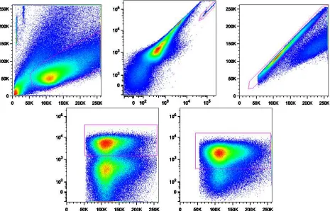
Figure 1: Typical gating procedure for flow cytometry data. Clockwise from top left: Lymphocytes are identified based upon size (forward scattered light, horizontal axis) and granularity (side scattered light, vertical axis); beads are identified by their fluorescence properties in the PE (horizontal axis) and FITC (vertical axis) channels; cell duplets are excluded by comparing the area (horizontal axis) and height (vertical axis) of the forward scattered light; CD3+ cells are identified; CD4+ cells are identified. Graphics prepared by C. Peligero.
cells by comparing the height (vertical axis) and area (horizontal axis) of the FSC signal (top right). CD4+ lymphocytes are identified by their expression of CD3 (bottom left) and CD4 (bottom right) as measured by the light emitted from the fluorochromes attached to anti-CD3 and anti-CD4.
After gating, the remaining cells can be counted into bins based upon their measured CFSE expression and then presented as a histogram. Because the mass of CFSE within a cell divides approximately in half with each division, it is most convenient to use a logarithmic scale for CFSE FI. Letzrepresent the (continuous) logarithmic axis on which FI is measured (hence units ofzare log units of intensity, or log UI). Now consider some partition {zk} (1 ≤ k ≤K) of this axis. The histogram data consists of the ordered pairs (zkj, n
j
k), which represent the
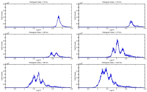
number of cellsnjk with measured FI in the interval [zk, zk+1) at timetj. Typical histogram data from a single
experiment are shown in Figure 2. Each ‘peak’ in the data represents a distinct generation of cells (i.e., cells in each peak have divided the same number of times since the beginning of the experiment). Because all cells (even in the absence of labelling by CFSE) have a natural brightness or autofluorescence, cells which have divided a sufficiently large number of times (typically 8-10 [70]) can no longer be distinguished from background noise in the flow cytometry data. In general, the effect of this detection limit is small as few cells are capable of completing this many divisions during a typical experiment.
0 0.5 1 1.5 2 2.5 3 3.5 0
0.5 1 1.5 2 2.5 3 3.5x 10
5 Histogram Data, t =0 hrs
Log FI
Cell Counts
0 0.5 1 1.5 2 2.5 3 3.5
0 0.5 1 1.5 2 2.5 3 3.5x 10
5 Histogram Data, t =24 hrs
Log FI
Cell Counts
0 0.5 1 1.5 2 2.5 3 3.5
0 0.5 1 1.5 2 2.5 3 3.5x 10
5 Histogram Data, t =48 hrs
Log FI
Cell Counts
0 0.5 1 1.5 2 2.5 3 3.5
0 0.5 1 1.5 2 2.5 3 3.5x 10
5 Histogram Data, t =72 hrs
Log FI
Cell Counts
0 0.5 1 1.5 2 2.5 3 3.5
0 0.5 1 1.5 2 2.5 3 3.5x 10
5 Histogram Data, t =96 hrs
Log FI
Cell Counts
0 0.5 1 1.5 2 2.5 3 3.5
0 0.5 1 1.5 2 2.5 3 3.5x 10
5 Histogram Data, t =120 hrs
Log FI
Cell Counts
Figure 2: Typical histogram representation of data from a CFSE-based proliferation assay. Originally from [56].
at each measurement time). Each measurement is obtained from a sample of a population of cells, and in fact, these samples are not drawn from the same population. (While all cells in the experiment are ultimately taken from the same donor, cells are harvested from physically distinct wells at each measurement time.) For almost all analysis and especially for mathematical modeling investigations, it is routinely and tacitly assumed that each well contains a population of cells which is identical to the populations in all other wells at all times. Moreover, only a fraction of the contents of each well is assessed by the flow cytometer. The measured fraction is estimated as the fraction of counted calibration beads to the known total number of beads. It is tacitly assumed that the sample drawn from each well is representative of the total contents of that well, and that the fraction of the well measured is accurately estimated by the bead scaling factor. In the context of a histogram representation of the measured cells, one can obtain an approximate population level histogram by scaling the numbers of cells counted into each bin by the reciprocal of the fraction of beads counted.
[79, Ch. 4].
Given the assumptions of the previous two paragraphs (wells contain identical populations of cells, the fraction of measured cells is representative of the well population, that fraction is exactly knowable, and gates accurately select a population of interest at each measurement time) one is able to treat a series of histograms resulting from flow cytometry measurements as if those histograms represent a complete census of a single population of cells at each measurement time. Of course, such a treatment is only accurate to the extent that the assumptions are valid. In actual fact, there are small differences (e.g., initial cell number) between populations of cells in distinct wells. Both the scaling factors (computed from the numbers of beads counted) and the gating procedures are subject to some error. Typically, all such errors are small and make minimal difference in the outcome of the experiment (and, in particular, in the calibration of a mathematical model). We emphasize that the assumptions which must be made in order to obtain histogram data are not indicative of any experimental shortcoming, but represent necessary steps to obtain meaningful data from a complex experimental setup. For the moment, the standard assumption will be made that histogram data (such as that in Figure 2) can be treated as census data. Shortcomings resulting from this assumption have been addressed in [79, Ch. 4] and will be highlighted at the end of this report.
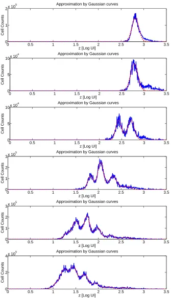
Given the histogram data in Figure 2, we return to the original goal of determining the number of cells having divided a given number of times. One simple method of obtaining this information is interval gating, in which the horizontal axis (FI) is partitioned into intervals which are assumed to correspond to particular numbers of divisions undergone. For instance, the data at t = 48 hours in Figure 2 might be partitioned at z = 2.55 so that cells with FI z ≤ 2.55 are assumed to have divided once while cells with FI z > 2.55 are assumed to be undivided. While this technique is quite simple, there is a clear shortcoming in that peaks corresponding to distinct generations of cells slightly overlap as a result of inhomogeneity in the initial labeling process. A less arbitrary and hopefully more accurate method to compute cell numbers is to fit each histogram with a series of gaussian-type curves. Consider the family of functions
φji(z) =Cijexp (z−µ
j
i)2
2(σij)2
!
.
The parametersCij, µ j i, andσ
j
i correspond (approximately) to the height, mean, and variance in the histogram
data of the cohort of cells having completed i divisions at time tj. These parameters can be determined by
minimizing the least squares cost functional
Oj=X
i
X
k,j
1
wjk
φji(zk)−njk
2
(1)
where wkj are weighting terms to account for the variance of the noisy histogram data points. While some work has focused on these weighting terms [79, 84], a complete statistical model is not known so that one typically useswkj = 1 for allj andk(ordinary least squares). Any similar parameter estimation technique (weighted least squares, likelihood estimation) would also suffice. Alternatively, approximate locations of each peak of cells can be determined using two experimental controls: one for unstimulated cells (which remain undivided) and one for unlabeled cells. See [58, Secs. B,C] for details. Typical results are shown (for the data from Figure 2) in Figure 3. One can then determine the number of cells ˆNij having dividedi times at measurement timetj by computing
ˆ
Nij =X
k
φji(zk).
0 0.5 1 1.5 2 2.5 3 3.5 0
1 2x 10
5 Approximation by Gaussian curves
z [Log UI]
Cell Counts
0 0.5 1 1.5 2 2.5 3 3.5
0 5 10x 10
4 Approximation by Gaussian curves
z [Log UI]
Cell Counts
0 0.5 1 1.5 2 2.5 3 3.5
0 5 10x 10
4 Approximation by Gaussian curves
z [Log UI]
Cell Counts
0 0.5 1 1.5 2 2.5 3 3.5
0 1 2 3x 10
5 Approximation by Gaussian curves
z [Log UI]
Cell Counts
0 0.5 1 1.5 2 2.5 3 3.5
0 1 2 3x 10
5 Approximation by Gaussian curves
z [Log UI]
Cell Counts
0 0.5 1 1.5 2 2.5 3 3.5
0 2 4x 10
5 Approximation by Gaussian curves
z [Log UI]
Cell Counts
Time (hrs)
Divisions 0 24 32 48 56 66 75 85
0 50000 14807 9160 1777 429 35 2 0
1 0 527 1861 3920 2351 541 65 3
2 0 75 560 5191 6501 3762 1045 104
3 0 3 66 2731 7161 10401 6627 1672
4 0 0 1 566 3129 11457 16710 10603
5 0 0 0 44 537 5006 16787 26736
6 0 0 0 0 33 859 6684 26859
7 0 0 0 0 0 52 1044 10695
8 0 0 0 0 0 0 54 1671
Table 1: Typical data for cell numbers computed from a histogram of CFSE data. Originally from [47].
3
Mathematical Models
One can clearly see in Figure 2 and in Table 1 that cell division is an asynchronous process. That is, there is a high degree of variability in the times at which cells divide so that multiple generations of cells are present in the population at any given time. The largest source of this asynchrony is generally considered to be the length of time taken for cells to enter the first division [43, 71], which is typically much longer than the time required for subsequent divisions as a result of the time required for initial activation of the cells. It has been shown that many mathematical models of cell division can be placed into one of two classes based upon how the source of this asynchrony is identified and mathematized [54]. The first class of models are consistent with the assumption that asynchrony is the result of inherent stochasticity in the intracellular machinery governing cell growth and division, so that cell division time is distributed in the population of cells under study. The second class of models can be derived from an assumption that population heterogeneity is the result of a deterministic cell interacting randomly with its environment. In the present context, the accuracy of either class of models can only be assessed in terms of accuracy in describing cell counts (e.g., Table 1). Unfortunately, such data alone is insufficient to reach any conclusions regarding which of the two classes of models is more accurate [54]. As such, the discussion below groups mathematical models not by underlying assumptions but rather by the manner in which cell cycle dynamics are modeled.
We remark that the dilemma of how to incorporate asynchrony and variability into “growth” models is not unique to cell proliferation; how to mathematically formulate variability in other growth processes such as marine populations (mosquitofish, shrimp) involving individual deterministic mechanisms in a variable environment vs. individual stochastic mechanisms has been treated specifically in [4, 11, 12, 25] as well as more generically in [9, 10, 16, 17]. While probability and stochasticity is fundamental to all of these models, the mathematical constructs used to incorporate asynchrony/variability into the modeling is strikingly different conceptually and computationally.
3.1
Random Birth-Death Models
The simplest class of models used to describe cellular division dynamics are random birth-death models which describe the processes of division and death with exponential rates. Such models follow from the assumption that times to divide and die are independent, exponential random variables. Let Ni(t) be the total number of cells
having completed i divisions at time t. Let αbe the (exponential) rate at which cells divide, and let β be the (exponential) rate at which cells die. Then a simple RBD model for cell numbers per generation is an autonomous system of ordinary differential equations (ODEs),
dN0
dt =−(α+β)N0(t) dNi
dt =−(α+β)Ni+ 2αNi−1(t), (2) with solution
N0(t) =N0(0)e−(α+β)t
Ni(t) =
(2αt)i
i! N0(t).
Such a model has been applied to cell numbers obtained from CFSE data by Revy et al., [72]. Given the values of Ni(tj) at measurement times tj and the data ˆNij (cf. Table 1), one can estimate the parameters (α, β) in an
ordinary least squares (OLS) framework similar to Equation (1). It follows that the average times to division and death are 1/αand 1/β, respectively.
Interestingly, the model (2) is also amenable to an alternative method of parameter estimation originally defined by the Hodgkin lab [43]. The discussion below follows the analysis of De Boer and Perelson [36]. Define
Pi(t) =Ni(t)/2i
to be the number of precursors (this terminology is widely used and perhaps sometimes without sufficient care in the literature–see [73] for a cogent discussion!) for the cells in generation i at timet (allowing for fractional precursors). It follows that
P0(t) =N0(t)
Pi(t) =
(αt)i
i! N0(t).
Note that the precursors at timetindicate the lines of proliferating cells that originated from a given cell originally in the population at time t= 0. The total number of precursors at timet is
P(t) =X
i
Pi(t) =N0(0)e
−(α+β)t X
i
(αt)i
i!
!
=N0(0)e −βt
. (3)
Finally, the normalized precursor frequency for generationiis
Pi(t)
P(t) = (αt)i
i! e −αt
,
which is a Poisson process with mean αt [36]. It follows that a graph of the Poisson processPi(t)/P(t) versus
i will appear normal for sufficiently large t [35] and the mean of this distribution will increase linearly in time with rate α. Given data ˆNij, one can compute precursor data ˆPij= ˆNij/2i. It is shown by Hodgkin et al., that,
Of course, the model (2) is generally too simple to accurately describe most proliferation assay data. How-ever, several extensions and generalizations have been proposed [36]. For instance, it has been observed that experimental data typically exhibit a delay between activation and the onset of proliferation [33]. This can easily be modeled as an initial transient of length τ,
dN0
dt =
−βN0(t), 0≤t≤τ −(α+β)N0(t), t > τ
dNi
dt =
0, 0≤t≤τ
−(α+β)N0(t) + 2αNi−1(t), t > τ
. (4)
Additionally, one can explicitly incorporate the fraction, φ, of cells which divides by writing
dN0
dt =
−βN0(t), 0≤t≤τ −(αφ+β)N0(t), t > τ
dN1
dt =
0, 0≤t≤τ
−(α+β)N1(t) + 2αφN0(t), t > τ
dNi
dt =
0, 0≤t≤τ
−(α+β)N0(t) + 2αφNi−1(t), t > τ
. (5)
Alternatively, studies of cell proliferation and death have long recognized that the gross behavior of a population differs greatly between divided and undivided cells [54]. Thus one could also consider the heterogeneous model [36]
dN0
dt =−(α0+β0)N0(t) dN1
dt =−(α+β)N1(t) + 2α0N0(t) dNi
dt =−(α+β)Ni(t) + 2αNi−1(t). (6)
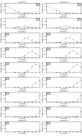
Mathematical analysis [36] has shown how the parameters of the models (4)–(6) can be identified from graphical data in a manner similar to that proposed by Gett and Hodgkin [43]. The primary advantage of such a graphical fitting method is that it does not require any complex mathematics or nonlinear optimization software. Biolog-ically relevant parameters are readily determined from simple computations and graphs of the data. In general, the primary shortcomings of such a parameter estimation procedure are tied to the shortcomings of the ODE system which motivates it.
0 24 32 48 56 66 75 85 2.0e+04
4.0e+04 6.0e+04
Time [hrs]
Number of Cells
Generation 0
Model Data
0 24 32 48 56 66 75 85 2.0e+04
4.0e+04 6.0e+04
Time [hrs]
Number of Cells
Generation 0
Model Data
0 24 32 48 56 66 75 85 2.0e+04
4.0e+04 6.0e+04
Time [hrs]
Number of Cells
Generation 0
Model Data
0 24 32 48 56 66 75 85 5.0e+03
1.0e+04 1.5e+04
Time [hrs]
Number of Cells
Generation 1
Model Data
0 24 32 48 56 66 75 85 5.0e+03
1.0e+04 1.5e+04
Time [hrs]
Number of Cells
Generation 1
Model Data
0 24 32 48 56 66 75 85 5.0e+03
1.0e+04 1.5e+04
Time [hrs]
Number of Cells
Generation 1
Model Data
0 24 32 48 56 66 75 85 4.0e+03
8.0e+03 1.2e+04
Time [hrs]
Number of Cells
Generation 2 Model
Data
0 24 32 48 56 66 75 85 4.0e+03
8.0e+03 1.2e+04
Time [hrs]
Number of Cells
Generation 2 Model
Data
0 24 32 48 56 66 75 85 4.0e+03
8.0e+03 1.2e+04
Time [hrs]
Number of Cells
Generation 2 Model
Data
0 24 32 48 56 66 75 85 5.0e+03
1.0e+04 1.5e+04
Time [hrs]
Number of Cells
Generation 3 Model
Data
0 24 32 48 56 66 75 85 5.0e+03
1.0e+04 1.5e+04
Time [hrs]
Number of Cells
Generation 3 Model
Data
0 24 32 48 56 66 75 85 5.0e+03
1.0e+04 1.5e+04
Time [hrs]
Number of Cells
Generation 3 Model
Data
0 24 32 48 56 66 75 85 6.7e+03
1.3e+04 2.0e+04
Time [hrs]
Number of Cells
Generation 4 Model
Data
0 24 32 48 56 66 75 85 6.7e+03
1.3e+04 2.0e+04
Time [hrs]
Number of Cells
Generation 4 Model
Data
0 24 32 48 56 66 75 85 6.7e+03
1.3e+04 2.0e+04
Time [hrs]
Number of Cells
Generation 4 Model
Data
0 24 32 48 56 66 75 85 1.3e+04
2.7e+04 4.0e+04
Time [hrs]
Number of Cells
Generation 5 Model
Data
0 24 32 48 56 66 75 85 1.3e+04
2.7e+04 4.0e+04
Time [hrs]
Number of Cells
Generation 5 Model
Data
0 24 32 48 56 66 75 85 1.3e+04
2.7e+04 4.0e+04
Time [hrs]
Number of Cells
Generation 5 Model
Data
0 24 32 48 56 66 75 85 1.3e+04
2.7e+04 4.0e+04
Time [hrs]
Number of Cells
Generation 6 Model
Data
0 24 32 48 56 66 75 85 1.3e+04
2.7e+04 4.0e+04
Time [hrs]
Number of Cells
Generation 6 Model
Data
0 24 32 48 56 66 75 85 1.3e+04
2.7e+04 4.0e+04
Time [hrs]
Number of Cells
Generation 6 Model
Data
0 24 32 48 56 66 75 85 6.7e+03
1.3e+04 2.0e+04
Time [hrs]
Number of Cells
Generation 7 Model
Data
0 24 32 48 56 66 75 85 6.7e+03
1.3e+04 2.0e+04
Time [hrs]
Number of Cells
Generation 7 Model
Data
0 24 32 48 56 66 75 85 6.7e+03
1.3e+04 2.0e+04
Time [hrs]
Number of Cells
Generation 7 Model
Data
0 24 32 48 56 66 75 85 5.0e+03
1.0e+04 1.5e+04
Time [hrs]
Number of Cells
Generation 8 Model
Data
0 24 32 48 56 66 75 85 5.0e+03
1.0e+04 1.5e+04
Time [hrs]
Number of Cells
Generation 8 Model
Data
0 24 32 48 56 66 75 85 5.0e+03
1.0e+04 1.5e+04
Time [hrs]
Number of Cells
Generation 8 Model
Data
3.2
Fixed-Cycle Models
One alternative to assuming an exponential distribution of times to divide and die (as is implicit in RBD models) is to assume a fixed cell cycle time for all cells in the population. Equivalently, one assumes that the time at which cells divide in any given generation is an atomic measure with a single unit mass (that is, it is a Dirac measure, so that all cells in a given generation divide after spending a fixed length of time in that generation). Of course, as noted previously, a population of activated cells does not undergo completely synchronous division. In keeping with the observation that the primary source of asynchrony within a dividing population is the time required to complete the first division, Deenick et al., [37] proposed a model in which the time to first division is normally distributed. Subsequent generations divide with a fixed cell cycle duration ∆. Cell death is again assumed to be independent of division and is described by an exponential distribution, with a parameterβ0 for undivided cells and a parameterβ for divided cells. A derivation of the resulting model can be found in [35] and can be written as an ODE-algebraic system
dN0
dt =− R(t)
2 −β0N0(t)
dN1
dt =R(t)−R(t−∆)e
−β∆
−βN1(t)
Ni(t) = 2e−β∆
i−1
N1(t−(i−1)∆). (7)
The function R(t) is a recruitment function describing the entry of cells into the first division. While Deenick et al. [37] propose a normal distribution, subsequent experiments using tritiated thymidine uptake have shown a lognormal distribution to be more accurate [53]. Thus the recruitment function is
R(t;µ, σ,∆0, C) =
C
√
2πσ(t−∆0) exp
−(log(t−∆0)−log(µ)) 2
2σ2
. (8)
The parametersµ andσ describe the mean and variance of the lognormal recruitment function, while ∆0 is an initial transient (so that the mean time to first division is µ+ ∆0. The parameterC= 2φN0, where N0 is the initial number of (undivided) cells in the population andφis the precursor fraction which indicates the number of cells which would have divided in the absence of cell death. The model (7) has been generalized to account for cell death which is heterogeneous with respect to the number of divisions undergone [52, 53] (for example, as a result of cell exhaustion). For generations i≥1, define the death rate parametersβi =β+m(i−1). Then a
generalization of (7) is
dNi
dt = 2
i−1
R(t−(i−1)∆)exp
−
i−1
X
j=1
βj∆
−2i
−1
R(t−i∆)exp
−
i
X
j−1
βj∆
−βiNi, (9)
fori≥2. The equations fori= 0 and i= 1 are unchanged.
0 24 32 48 56 66 75 85 2.0e+04
4.0e+04 6.0e+04
Time [hrs]
Number of Cells
Generation 0
Model Data
0 24 32 48 56 66 75 85 2.0e+04
4.0e+04 6.0e+04
Time [hrs]
Number of Cells
Generation 0
Model Data
0 24 32 48 56 66 75 85 5.0e+03
1.0e+04 1.5e+04
Time [hrs]
Number of Cells
Generation 1
Model Data
0 24 32 48 56 66 75 85 5.0e+03
1.0e+04 1.5e+04
Time [hrs]
Number of Cells
Generation 1
Model Data
0 24 32 48 56 66 75 85 4.0e+03
8.0e+03 1.2e+04
Time [hrs]
Number of Cells
Generation 2 Model
Data
0 24 32 48 56 66 75 85 4.0e+03
8.0e+03 1.2e+04
Time [hrs]
Number of Cells
Generation 2 Model
Data
0 24 32 48 56 66 75 85 5.0e+03
1.0e+04 1.5e+04
Time [hrs]
Number of Cells
Generation 3 Model
Data
0 24 32 48 56 66 75 85 5.0e+03
1.0e+04 1.5e+04
Time [hrs]
Number of Cells
Generation 3 Model
Data
0 24 32 48 56 66 75 85 6.7e+03
1.3e+04 2.0e+04
Time [hrs]
Number of Cells
Generation 4 Model
Data
0 24 32 48 56 66 75 85 6.7e+03
1.3e+04 2.0e+04
Time [hrs]
Number of Cells
Generation 4 Model
Data
0 24 32 48 56 66 75 85 1.3e+04
2.7e+04 4.0e+04
Time [hrs]
Number of Cells
Generation 5 Model
Data
0 24 32 48 56 66 75 85 1.3e+04
2.7e+04 4.0e+04
Time [hrs]
Number of Cells
Generation 5 Model
Data
0 24 32 48 56 66 75 85 1.3e+04
2.7e+04 4.0e+04
Time [hrs]
Number of Cells
Generation 6 Model
Data
0 24 32 48 56 66 75 85 1.3e+04
2.7e+04 4.0e+04
Time [hrs]
Number of Cells
Generation 6 Model
Data
0 24 32 48 56 66 75 85 6.7e+03
1.3e+04 2.0e+04
Time [hrs]
Number of Cells
Generation 7 Model
Data
0 24 32 48 56 66 75 85 6.7e+03
1.3e+04 2.0e+04
Time [hrs]
Number of Cells
Generation 7 Model
Data
0 24 32 48 56 66 75 85 5.0e+03
1.0e+04 1.5e+04
Time [hrs]
Number of Cells
Generation 8 Model
Data
0 24 32 48 56 66 75 85 5.0e+03
1.0e+04 1.5e+04
Time [hrs]
Number of Cells
Generation 8 Model
Data
3.3
Smith-Martin Models
Rather than consider a fixed cell cycle time ∆ which is constant for all cells in the population, one could instead assume some level of variability in cell cycle time. In many cases, mathematical formalisms of such cell cycle dynamics begin with the Smith-Martin [76] model, in which the cell cycle is divided into an A state and a B state. The A phase of the Smith-Martin model (which is approximately the G1 phase of the cell cycle) is assumed to have a stochastic duration so that cells may remain in the A phase indefinitely, but exit into the B phase with a fixed transition probability. Meanwhile the B phase (which is approximately the S, G2, and M phases of the cell cycle) is assumed to have a deterministic length after which cells divide and return to the A state. The Smith-Martin model thus imposes a minimum cell cycle time (the duration of the B state) while also allowing for variability in cycle lengths in the population of cells.
Nordon et al., [66] used a Smith-Martin model to account for precursor numbers for CFSE-based cytometry data and derived a set of biologically meaningful parameters which could be determined from graphical represen-tations of the data (cf., the method of Gett and Hodgkin [43]). A complete Smith-Martin model which accounts for total cell numbers computed from CFSE data can be derived from a coupled set of equations [29, 69]. As-sume the stochastic A phase has a duration which can be modeled as an exponential random variable. Then the transition of cells from the A state to the B state is modeled with an ordinary differential equation. The fixed duration of the B phase is then modeled with an age-structured partial differential equation in which all cells must progress from an initial age a= 0 (when cells enter the B phase from the A phase) to a final age a= ∆ (the duration of the B phase, at which time cells return to the A state). Let Ai(t) represent the total number
of cells having completed i divisions at timet and currently in the ‘A’ state. Let bi(t, s) be the age-structured
density (number per unit age) of cells having completedidivisions at timet and having spent timesin the ‘B’ state. Then the Smith-Martin model is
dAi(t)
dt =2bi−1(t,∆)−(α−βA)Ai(t)
∂bi
∂t + ∂bi
∂s =−βBbi(t, s) 0≤s≤∆ bi(t,0) =αAi(t),
whereαis the rate of transition from the A state to the B state andβAandβBare the (exponential) probabilities
of death in the two states. By convention,b−1(t, s) = 0 for allt, s. Trivially, the solution for the B phase is
bi(t, s) =αe−βBsAi(t−s), i≥0.
Hence it follows that the total number of cells having undergoneidivisions isNi(t) =Ai(t) +Bi(t) where
dAi
dt =−(α+βA)Ai(t) + 2αe
−βB∆
Ai−1(t−∆), i≥0
Bi(t) =
Z ∆
0
bi(t, s)ds=α
Z ∆
0
e−βBs
Ai(t−s)ds, (10)
where it is assumed thatA−1(t) = 0 for allt. It should be noted that one may alternatively compute the number of cells in the B phase as [41]
dBi(t)
dt =αAi(t)−αe
−βB∆
Ai(t−∆)−βBBi(t).
It is assumed that all cells are in stateA0att= 0 hours. Given the nature of the two phases of the Smith-Martin model (an A phase with an exponentially distributed duration, and a B phase with a constant duration), it is accurate to think of the Smith-Martin model as a generalization of both RBD models and fixed-cycle models. In fact, it can be shown [69, Appendix] that the homogeneous fixed cycle model (7) is equivalent to a Smith Martin model with no A state. The age-structured PDE then has the new boundary condition bi(t, s) = 2bi−1(t,∆). Similarly, the homogeneous ODE model (2) is obtained in the limit as ∆→0, providedβA=βB=β. However,
is clear that the manner in which death is modeled within the cell cycle is of fundamental importance for the accurate estimation of parameters. Unfortunately, the parametersβAandβB cannot be simultaneously estimated
(uniquely) without additional data such as the fraction of cells in division [42]. This lack of identifiability is common to both direct (least squares) estimation and indirect/graphical methods for parameter estimation. In this summary it will be assumed thatβA=βB as this is most closely associated with RBD models for purposes
of comparison. However, it should be carefully noted that such an assumption may not necessarily accurately reflect the actual underlying dynamics [69].
The Smith-Martin model has been shown to much more accurately describe cell counts obtained from CFSE data when compared to RBD models, perhaps as the result of the minimum cell cycle time [36] (as was observed with the fixed-cycle models). In keeping with the observation that the first division after activation typically takes much longer than subsequent divisions, a generalization of the Smith-Martin model can allow for heterogeneous (with respect to the number of divisions undergone) transition rates and cell cycle times. The resulting model is
dA0(t)
dt =−(α0+β0)A0(t) dA1(t)
dt =−(α+βA)A1(t) + 2α0A0(t−∆0)e
−βB∆0
dAi(t)
dt =−(α+βA)Ai(t) + 2αAi−1(t−∆)e
βB∆
.
B0(t) =α0
Z ∆0
0
A0(t−s)e−βBsds
Bi(t) =α
Z ∆
0
Ai(t−s)e−βBsds. (11)
As before, the total number of cells in each generation isNi(t) =Ai(t) +Bi(t). Another possible generalization
of the Smith-Martin model uses a recruitment function (cf. the fixed-cycle models (7) and (9)) to describe the transition of cells from the initialA0 state to theB0 state. The resulting model is
dA0(t)
dt =−β0A0(t)− R(t)
2
dA1(t)
dt =−(α+β)A1(t) +R(t). (12)
The Ai(t), i≥2 and Bi(t), i≥0 are computed exactly as in (11). Lee and Perelson discuss both a lognormal
distribution and a delayed gamma distribution to describe the recruitment function R(t). While the delayed gamma distribution can be derived from assumptions regarding a two-step activation process and permits the analytic solution of the model, the authors find that a lognormal distribution (8) is a more accurate description of cellular activation as measured by thymidine incorporation [53] and that is what is used here. The Smith-Martin model can be generalized further by considering a cell death rate which increases with division number,
βi=β+ (i−1)m, fori≥1 [41, 53] or by considering a B phase duration which increases with division number,
∆n= ∆ + (i−1)m[53].
of increasing cell death with division number or increasing division time improve the model similarly [53], with slightly more improvement arising from increasing cell death [52].
3.4
Probabilistic Models
As discussed above, the classical Smith-Martin model is consistent with the assumption that the probability of division is exponentially distributed with a delay while time to death is exponentially distributed. Yet it is also clear from Figure 6 that a generalized Smith-Martin model, in which the first division is described by a lognormal recruitment process, is much more accurate in describing the data from Table 1. An obvious question, then, is whether such probabilistic structures can be used more generally to describe rates of division and death within a population of cells. Using observations obtained from several experiments, Hawkins et al., [48] show that the apparently random nature of the mechanisms of cell division and death is consistent with the hypothesis that the cellular controls of those processes operate independently of one another. Thus the time to divide and time to die of an individual cell can be thought of as independent random variables; after each division, a single cell receives one realization of each random variable, and the fate of the cell is determined by the minimum of the two realizations. Hawkins et al., propose the name ‘cyton’ for this regulatory mechanism [47]. It is assumed that division times are not inherited from the previous generation, and that sibling cells are independent of one another. It follows that the expected number of cells having undergone a specified number of divisions at a given time can be determined from the probability distributions from which the times to divide and die are drawn, given the initial number of cells in the population.
In most general terms, the cyton model computes the number of cells having undergoneidivisions at timet
as
Ni(t) = 2iN0
Z t
0
ri(τ)dτ −
Z t
0
di(τ)dτ−
Z t
0
ri+1(τ)dτ
,
whereri(t) is a density function describing the probability of cells entering theith generation at timet. Similarly,
di(t) is a density function describing the probability cells in generationidying at timet. Of course, the functions
ri(t) and di(t) will depend upon the corresponding functions for all prior generations of cells [52]. As a result,
these density functions are typically defined via convolution integrals [52, 54]. With appropriate choice of the functionsri(t) anddi(t), it can be shown that the cyton model is a generalization of both fixed-cycle models and
Smith-Martin models [52, 54].
While the formulation above is quite general, the original formulation of the cyton model by Hawkins et al. [33, 47] is more intuitive. For cells having undergoneidivisions, consider the numbers of cellsndiv
i (t) andndiei (t)
having undergoneidivisions that divide and die, respectively, at timet. For undivided cells, these functions can be specified as
ndiv
0 (t) =F0N0
1−
Z t
0
ψ0(s)ds
φ0(t)
ndie
0 (t) =N0
1−F0
Z t
0
φ0(s)ds
ψ0(t), (13)
where φ0(t) and ψ0(t) are density functions for the probability that undivided cells divide and die, respectively.
F0 is the fraction of undivided cells which would (in the absence of cell death) progress to the next generation. For theith division class, let the functionsφ
i(t) andψi(t) be density functions which characterize the probability
of division and death, respectively, and let Fi be the progressor fraction. Then for subsequent generations we
have
ndiv
i (t) = 2Fi
Z t
0
ndiv
i−1(s)
1−
Z t−s 0
ψi(ξ)dξ
φi(t−s)ds
ndiei (t) = 2
Z t
0
ndivi−1(s)
1−Fi
Z t−s
0
φi(ξ)dξ
0 24 32 48 56 66 75 85 2.0e+04
4.0e+04 6.0e+04
Time [hrs]
Number of Cells
Generation 0
Model Data
0 24 32 48 56 66 75 85 2.0e+04
4.0e+04 6.0e+04
Time [hrs]
Number of Cells
Generation 0
Model Data
0 24 32 48 56 66 75 85 5.0e+03
1.0e+04 1.5e+04
Time [hrs]
Number of Cells
Generation 1
Model Data
0 24 32 48 56 66 75 85 5.0e+03
1.0e+04 1.5e+04
Time [hrs]
Number of Cells
Generation 1
Model Data
0 24 32 48 56 66 75 85 4.0e+03
8.0e+03 1.2e+04
Time [hrs]
Number of Cells
Generation 2 Model
Data
0 24 32 48 56 66 75 85 4.0e+03
8.0e+03 1.2e+04
Time [hrs]
Number of Cells
Generation 2 Model
Data
0 24 32 48 56 66 75 85 5.0e+03
1.0e+04 1.5e+04
Time [hrs]
Number of Cells
Generation 3 Model
Data
0 24 32 48 56 66 75 85 5.0e+03
1.0e+04 1.5e+04
Time [hrs]
Number of Cells
Generation 3 Model
Data
0 24 32 48 56 66 75 85 6.7e+03
1.3e+04 2.0e+04
Time [hrs]
Number of Cells
Generation 4 Model
Data
0 24 32 48 56 66 75 85 6.7e+03
1.3e+04 2.0e+04
Time [hrs]
Number of Cells
Generation 4 Model
Data
0 24 32 48 56 66 75 85 1.3e+04
2.7e+04 4.0e+04
Time [hrs]
Number of Cells
Generation 5 Model
Data
0 24 32 48 56 66 75 85 1.3e+04
2.7e+04 4.0e+04
Time [hrs]
Number of Cells
Generation 5 Model
Data
0 24 32 48 56 66 75 85 1.3e+04
2.7e+04 4.0e+04
Time [hrs]
Number of Cells
Generation 6 Model
Data
0 24 32 48 56 66 75 85 1.3e+04
2.7e+04 4.0e+04
Time [hrs]
Number of Cells
Generation 6 Model
Data
0 24 32 48 56 66 75 85 6.7e+03
1.3e+04 2.0e+04
Time [hrs]
Number of Cells
Generation 7 Model
Data
0 24 32 48 56 66 75 85 6.7e+03
1.3e+04 2.0e+04
Time [hrs]
Number of Cells
Generation 7 Model
Data
0 24 32 48 56 66 75 85 5.0e+03
1.0e+04 1.5e+04
Time [hrs]
Number of Cells
Generation 8 Model
Data
0 24 32 48 56 66 75 85 5.0e+03
1.0e+04 1.5e+04
Time [hrs]
Number of Cells
Generation 8 Model
Data
Model Description # Params OLS Cost AIC AIC Diff
RBD1 Homogeneous ODE; (2) 2 1.9159×10
9
1091.51 374.70 RBD2 RBD1 with initial transient; (4) 3 1.1667×10
9
1062.26 345.45 RBD3 RBD2 with progressor fraction; (5) 4 1.1667×10
9
1064.26 347.45
RBD4 Heterogeneous ODE; (6) 4 9.9388×10
8
1054.16 337.35 Fixed-Cycle1 Lognormal recruitment, fixed cycle time; (7) 7 4.6761×10
7
867.60 150.79 Fixed-Cycle2 Fixed-Cycle1 with increasing death; (9) 8 3.3363×10
7
848.33 131.52 SM1 Classical Smith-Martin model; (10) 3 2.3748×10
9
1107.04 390.23 SM2 SM1 with different divided/undivided rates; (11) 6 1.5218×10
9
1085.00 368.19 SM3 SM2 with lognormal recruitment into first division; (12) 8 2.1772×10
7
821.44 104.63 SM4 SM3 with linearly increasing death 9 2.0506×10
7
819.66 102.85 SM5 SM3 with linearly increasing cycle length 9 2.1116×10
7
821.51 104.70 Cyton1 Lognormal distributions, no death for divided cells 6 3.8969×10
7
854.11 137.30 Cyton2 Cyton1 with a progressor fraction 7 3.0204×10
7
840.06 123.25 Cyton3 Cyton1 with lognormal death for undivided cells 8 4.1363×10
6
716.81 – Cyton4 Cyton 3 with a progressor fraction 9 4.1363×10
6
718.81 2.00
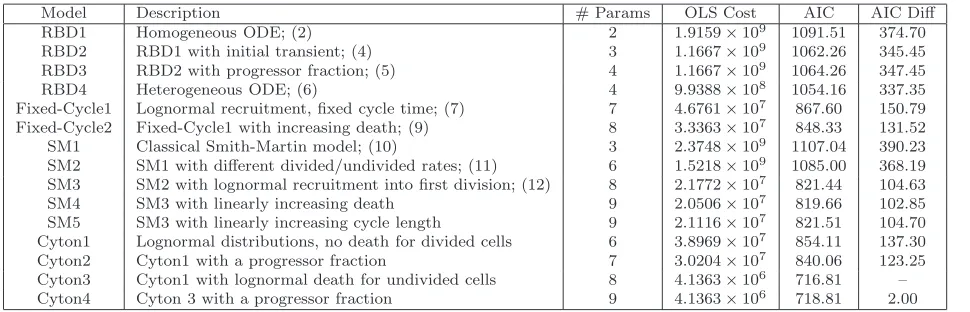
Table 2: Summary of mathematical models for describing cell numbers per generation. The OLS cost and Akaike Information Criteria (AIC) [32] are provided, as well as the AIC differences (difference between an AIC value and the smallest AIC value of all the models tested). The model with the minimum AIC value is considered the information-theoretic best model. Models with AIC differences greater than 10 (hence all models other than the cyton model) are considered to be significantly inferior based upon the given data set. The results above are consistent with those of [47].
Finally, one can compute the cell numbers
N0(t) =N0−
Z t
0
ndiv
0 (s)−ndie0 (s)
ds
Ni(t) =
Z t
0 2ndiv
i−1(s)−n
div
i (s)−ndiei (s)
ds. (15)
Thus the progression of a population of cells through several rounds of division, with the possibility of dying, as well as the variability inherent in that progression, is described by the ‘cytons’ {φi(t), ψi(t)} which specify
the probability (in time) of division and death for cells having undergone i divisions, as well as the progressor fractionsFi.
Typically, it is assumed that functions φi(t) and ψi(t) are lognormal density functions and thus can be
described by two parameters, a mean and a variance. In our summary here it will be assumed that undivided cells are characterized by a cyton{φ0(t), ψ0(t)}and divided cells are characterized by a separate cyton{φ(t), ψ(t)} for all i≥1. For the simplest model, it is assumed that Fi = 1 for alli and that death is negligible for divided
cells. (This can be accomplished either by setting ψ(t) = 0, or assigning ψ(t) with sufficiently large mean and sufficiently small variance so that essentially all cells have divided before there is any probability of dying.) This simple model can be generalized by including an initial progressor fractionF0≤1 (butFi = 1 still for alli≥1).
Each of these two models can in turn be generalized by including a nonnegligible probability of death for divided cells. The best fit results of these cyton models are summarized in Table 2. It seems clear from that table that death cannot be ignored among divided cells, a hypothesis further support by the fits to data in Figure 7.
It is clear from Figure 7 that the cyton model is an accurate description of the given data set. In fact, it outperforms all other models tested and does not require a significantly larger number of parameters (see Table 2). Moreover, the probability density functions φi(t) and ψi(t) allow for intuitive interpretations of the calibrated
0 24 32 48 56 66 75 85 2.0e+04
4.0e+04 6.0e+04
Time [hrs]
Number of Cells
Generation 0
Model Data
0 24 32 48 56 66 75 85 2.0e+04
4.0e+04 6.0e+04
Time [hrs]
Number of Cells
Generation 0
Model Data
0 24 32 48 56 66 75 85 5.0e+03
1.0e+04 1.5e+04
Time [hrs]
Number of Cells
Generation 1
Model Data
0 24 32 48 56 66 75 85 5.0e+03
1.0e+04 1.5e+04
Time [hrs]
Number of Cells
Generation 1
Model Data
0 24 32 48 56 66 75 85 4.0e+03
8.0e+03 1.2e+04
Time [hrs]
Number of Cells
Generation 2 Model
Data
0 24 32 48 56 66 75 85 4.0e+03
8.0e+03 1.2e+04
Time [hrs]
Number of Cells
Generation 2 Model
Data
0 24 32 48 56 66 75 85 5.0e+03
1.0e+04 1.5e+04
Time [hrs]
Number of Cells
Generation 3 Model
Data
0 24 32 48 56 66 75 85 5.0e+03
1.0e+04 1.5e+04
Time [hrs]
Number of Cells
Generation 3 Model
Data
0 24 32 48 56 66 75 85 6.7e+03
1.3e+04 2.0e+04
Time [hrs]
Number of Cells
Generation 4 Model
Data
0 24 32 48 56 66 75 85 6.7e+03
1.3e+04 2.0e+04
Time [hrs]
Number of Cells
Generation 4 Model
Data
0 24 32 48 56 66 75 85 1.3e+04
2.7e+04 4.0e+04
Time [hrs]
Number of Cells
Generation 5 Model
Data
0 24 32 48 56 66 75 85 1.3e+04
2.7e+04 4.0e+04
Time [hrs]
Number of Cells
Generation 5 Model
Data
0 24 32 48 56 66 75 85 1.3e+04
2.7e+04 4.0e+04
Time [hrs]
Number of Cells
Generation 6 Model
Data
0 24 32 48 56 66 75 85 1.3e+04
2.7e+04 4.0e+04
Time [hrs]
Number of Cells
Generation 6 Model
Data
0 24 32 48 56 66 75 85 6.7e+03
1.3e+04 2.0e+04
Time [hrs]
Number of Cells
Generation 7 Model
Data
0 24 32 48 56 66 75 85 6.7e+03
1.3e+04 2.0e+04
Time [hrs]
Number of Cells
Generation 7 Model
Data
0 24 32 48 56 66 75 85 5.0e+03
1.0e+04 1.5e+04
Time [hrs]
Number of Cells
Generation 8 Model
Data
0 24 32 48 56 66 75 85 5.0e+03
1.0e+04 1.5e+04
Time [hrs]
Number of Cells
Generation 8 Model
Data
3.5
Label-Structured PDE Models
Each of the models discussed thus far has been used effectively to provide various measures of the proliferative capacity of a population of cells. The cyton model in particular is capable of describing with considerable accuracy the time evolution of the generation structure of a population of dividing cells. Of course, validation of such models is based upon cell numbers computed from CFSE histogram data as discussed in Section 2. While such approaches are common and easy to implement, the particular functions (e.g., gaussian densities) might lead to biased computation of cell numbers, particularly if the division peaks in the histogram data are not well-resolved. Thus, there seems to be an advantage in the direct mathematical modeling of CFSE histogram data. To this end, structured population models have been proposed [21, 22, 55, 56, 79]. Such partial differential equation (PDE) models have long been discussed in the context of cell populations [28] and can be structured by age [1, 27, 39, 44], cyclin content [27], size [40, 44, 45, 68] or DNA-content [26], or any number of other physiological variables [62].
Rather than using such physiologically-structured models, the histogram presentation of a cell population in terms of measured fluorescence intensity (Figure 2) makes fluorescence intensity a natural structure variable with which to model. The use of such a nonphysiological structure variable was suggested as early as 2000 for BrdU-based assays [30], and was first explored in the context of CFSE-based assays in [56]. More recent work [8, 21, 22, 55, 79] has consistently demonstrated that the label-structured PDE framework can accurately model the observed histogram data from a CFSE-based proliferation assay. The primary benefit of using such a model is the ability to treat CFSE histogram data directly. Though the reconstruction of CFSE profiles from computed cell numbers has been suggested [47, SI Text], a label-structured model is a more fundamental and more complex effort, as one must account for the intracellular dynamics of label dilution and turnover while simultaneously estimating proliferation and death dynamics at the population level. In return for this added difficulty, one can potentially avoid some issues of biased cell counts, particularly as this method should be less reliant on distinct peak separations in the CFSE histogram data [23, 79].
Letn(t, x) be the structured density (cell per unit of fluorescence intensity) of a population of cells at timet
and with measured FIx. Then this population density can be described by the PDE
∂n(t, x)
∂t −ce
−kt∂[(x−xa)n(t, x)]
∂x =−(α(t, x) +β(t, x))n(t, x)χ[xa,x∗]4α(t,2x−xa)n(t,2x−xa)
n(0, x) = Φ(x)
n(t, xmax) = 0
v(t, xa)n(t, xa) = 0. (16)
The functionsα(t, x) andβ(t, x) are the rates of cell division and death, respectively, in units 1/hr. The motivating idea for the structural dependence of these rates is that the dilution of CFSE by division allows one to relate measured FI to the number of divisions undergone. Thus the structural dependence of the division and death rate functions is a surrogate for division dependence. The parameterxa accounts for the autofluorescence or natural
brightness of unlabeled cells. The advection term in the equation above (with parameterscandk) models the slow decay of CFSE FI (as a result of the natural turnover of intracellular proteins within the cell) using a Gompertz decay process [21]. These two features (autofluorescence and label decay) are important mathematical structures describing the manner in which the intracellular dye is processed by cells. The densityn(t, x) can then be used to compute cell counts in terms of measured FI, to be compared directly to histogram data such as Figure 2.
While the model (16) has been shown to very accurately fit CFSE histogram data [21, 22], it cannot be used to compute quantities such as the number of cells having undergone a given number of divisions. As such, it is not (in the form above) directly comparable to the methods previously discussed. Also, though the structural dependence of the proliferation and death rate functions can be used to infer division-dependent characteristics [21, 79], this interpretation is neither straightforward nor intuitive [74]. In order to alleviate these difficulties, a simple reformulation [23, 46, 74, 79] of the model (16) can be used to describe the structured densities of subpopulations of cells corresponding to distinct generations, which interact through division. Letni(t, x) be the
0 0.5 1 1.5 2 2.5 3 3.5 0
2 4 6 8 10x 10
4 Calibrated Model, t =24hrs
Log UI
Cell Counts
Data Model
0 0.5 1 1.5 2 2.5 3 3.5
0 1 2 3 4 5 6 7 8 9x 10
4 Calibrated Model, t =48hrs
Log UI
Cell Counts
Data Model
0 0.5 1 1.5 2 2.5 3 3.5 0
0.5 1 1.5 2 2.5x 10
5 Calibrated Model, t =96hrs
Log UI
Cell Counts
Data Model
0 0.5 1 1.5 2 2.5 3 3.5 0
0.5 1 1.5 2 2.5 3 3.5x 10
5 Calibrated Model, t =120hrs
Log UI
Cell Counts
Data Model
Figure 8: Best-fit solution for model (17) to a particular data set. Data originally from [56].
Then the subpopulations are described by the system
∂n0
∂t −ce
−kt
(x−xa)
∂n0
∂x =−(α0(t) +β0(t)−ce
−kt
)n0(t, x)
∂n1
∂t −ce
−kt
(x−xa)
∂n1
∂x =−(α1(t) +β1(t)−ce
−kt
)n1(t, x) +R1(t, x) ..
.
∂nimax
∂t −ce
−kt
(x−xa)
∂nimax
∂x =−(βimax(t)−ce
−kt
)nimax(t, x) +Rimax(t, x), (17)
with boundary conditions given as in (16). The recruitment term, which as above assumes symmetric label division at mitosis, is given by Ri(t, x) = 4αi−1(t)ni−1(t,2x−xa). It is assumed that all cells are undivided at
t = 0, with some initial FIn0(0, x) = Φ(x). Several parameterizations of the division and death rate functions
αi(t) andβi(t) have been proposed [23], with best-fit results obtained when the division rates are piecewise-linear
functions of time and the death rates are constants, with both division and death rates depending upon the number of divisions undergone. It has also been shown [23, 79] that variability (among all cells in the population) in the autofluorescence parameter xa is a significant physical feature of an accurate mathematical model and
can be accurately modeled with a lognormal distribution [23, 46, 79]. The best-fit solution to model (17) for a particular data set (data originally from [56]) is shown in Figure 8 and demonstrates the suitability of the given model in describing data from CFSE-based proliferation assays.
Again, assuming symmetric division, the resulting model is
∂n0
∂t −ce
−kt∂xn0
∂x =−(α0(t) +β0(t))n0(t, x) ∂n1
∂t −ce
−kt∂xn1
∂x =−(α1(t) +β1(t))n1(t, x) + 4αi−1(t)ni−1(t,2x) (18) ..
.
The boundary conditions and initial condition are again given as in (16) and (17). The major advantage of this slight reformulation is the manner of solution. In keeping with the notation used in previous sections, define the initial and subpopulation cell numbers,
N0=
Z ∞ 0
Φ(x)dx
N0(t) =
Z ∞
0
n0(t, x)dx
N1(t) =
Z ∞
0
n1(t, x)dx ..
.
Then it can be shown [46, 74] that the solution to model (18) is given by
ni(t, x) =Ni(t)¯ni(t, x) (19)
for alli, where the functionsNi(t) satisfy the ODE system
dN0
dt =−(α0(t) +β0(t))N0(t) dN1
dt =−(α1(t) +β1(t))N1(t) + 2αi−1(t)Ni−1(t) (20) ..
.
with initial conditionsN0(0) =N0,Ni(0) = 0 for alli≥1, and the functions ¯ni(t, x) satisfy the PDE
∂n¯i(t, x)
∂t −ce
−kt∂[xn¯i(t, x)]
∂x = 0 (21)
with initial condition
¯
ni(0, x) =
2iΦ(2ix)
N0
.
Equation (21) can be solved analytically by the method of characteristics to obtain
¯
ni(t, x) = 2iexp
−c
k(1−e
−kt )Φ 2
iexp c
k(1−e
−kt )
x
N0
.
(in which xis fluorescence intensityresulting from CFSE) to the actual measured CFSE profiles (which include the contribution of autofluorescence); this can be done via convolution with a density kernel representing the distribution of AutoFI in the population, and fast approximation techniques have been established. Appropriate numerical approximation and convergence results have also been demonstrated in [46].
In addition to the speed with which a solution can be computed, the model formulation (18) and its associated method of solution are premised upon mathematically decoupling the mechanisms of cell division, intracellular processing of label mass, and measurement by flow cytometry. The result of [46] is a more intuitive model formulation which can be viewed as a unifying framework linking models of cell numbers (described in Sections 3.1–3.4) and models of label dynamics (Section 3.5). Ideas from [23, 46] have recently been combined with the cyton formulation [33, 47] (see also Section 3.4) to yield a conservation-based probabilistic model that provides an excellent fit to histogram data [24].
4
Concluding Remarks
This review began with an overview of the complex experimental procedure which is used to study the manner in which cells of the immune system respond to stimulation. Several significant issues regarding mathematical and statistical aspects of the data collection procedure were addressed there, but were subsequently given little attention as several mathematical models of dividing cell dynamics were discussed. The single assumption common to every mathematical model of cell dynamics is the treatment of flow cytometry measurements as a census of a single population of cells. As discussed previously, this assumption is reliable for most data sets and is perhaps unavoidable. Somewhat surprisingly there have been few detailed analyses of the mathematical and statistical implications of this most fundamental assumption.
The most significant implication of assuming a single population is being measured repeatedly is that subtle variations in the populations of distinct wells are indistinguishable from fluctuations in the total number of cells in the population at a given time. The same problem arises from using a small sample of each well and then scaling (which is subject to some error) to estimate the total population. For instance, one can end up with more cells in a population at a given measurement time than would be physically possible given the preceding measurement [21, 35, 51, 79]. Of equal importance, parameters of a mathematical model (rates of cell death, in particular) may be incorrectly inferred, or confidence intervals on parameters may be too small if such issues are not taken into account. Some effort has been directed toward formulating an accurate statistical model of data from CFSE based proliferation assays, both for cell numbers computed from histogram data [84] and for the histogram data itself [50, 79].
In Sections 3.1–3.4, numerous mathematical models are summarized which describe the dynamics of a division-structured population of cells. Each of these models has been fit to a typical cell count data set (Table 1) and the results are summarized in Table 2, along with the associated AIC values for model comparison. This was done with recognition that the AIC is only a suggestive statistic and conditions [32] for AIC to be a rigorous approximation are not met. Nonetheless, based upon this table, the cyton model is strongly supported as providing the best description of cell division dynamics. On one hand, this is not surprising as the cyton model can be considered a generalization of the other models tested. In spite of this generality, the cyton model is based upon a simple premise (times to division and death) which is readily relatable to biologically meaningful parameters. On the other hand, care must be taken to avoid overreaching conclusions given only a single data set, in addition to the uncertainties just discussed regarding the statistical model and the AIC criteria.
![Table 1: Typical data for cell numbers computed from a histogram of CFSE data. Originally from [47].](https://thumb-us.123doks.com/thumbv2/123dok_us/1560368.1191643/9.612.159.486.57.193/table-typical-data-numbers-computed-histogram-cfse-originally.webp)
![Figure 4: OLS best-fit results for several RBD models.Left: Homogeneous ODE model (2) [72].Middle:Homogeneous ODE model with initial transient and precursor fraction (5) [36].Right: Heterogeneous ODEmodel (6) [36]](https://thumb-us.123doks.com/thumbv2/123dok_us/1560368.1191643/12.612.83.563.76.590/figure-homogeneous-homogeneous-transient-precursor-fraction-heterogeneous-odemodel.webp)
![Figure 5: OLS best-fit results for two fixed-cycle models.Left: Homogeneous Deenick model (7) [37] withlognormal recruitment function (8)](https://thumb-us.123doks.com/thumbv2/123dok_us/1560368.1191643/14.612.161.484.82.603/figure-results-xed-homogeneous-deenick-withlognormal-recruitment-function.webp)

![Figure 8: Best-fit solution for model (17) to a particular data set. Data originally from [56].](https://thumb-us.123doks.com/thumbv2/123dok_us/1560368.1191643/22.612.102.543.59.340/figure-best-t-solution-model-particular-data-originally.webp)