ABSTRACT
SUAREZ, VINICIO. Implementation of Direct Displacement Based Design for Pile and
Drilled Shaft Bents. (Under the direction of Dr. Mervyn Kowalsky)
The work in this thesis attempts to implement the Direct Displacement Based Design
(DDBD) method to the seismic design of long reinforced concrete pile and drilled shaft bents
embedded in soft soils. DDBD has been successfully used to design bridge columns that are
fixed at ground level and without soil interaction. The implementation of DDBD for column
bents, however, requires the consideration of soil-structure interaction effects--namely added
flexibility and damping. The main objective of this research is to develop an equivalent
model to predict yield displacement and ductility and to assess the equivalent viscous
damping as a function of ductility demand and soil type.
The proposed equivalent cantilever model replaces a nonlinear soil-column system.
In the equivalent model, the column is considered fixed at some depth below ground at the
point of maximum moment and possible formation of an underground plastic hinge. The
yield displacement of the column is matched with the yield displacement of the soil-column
model by introducing a coefficient and the energy dissipation characteristics are matched by
the introduction of equivalent viscous damping as function of ductility and soil type. Charts
and equations are provided to compute all the parameters involved in the equivalent
formulation. These aids resulted from parametric studies that involved nonlinear static and
Biography
Vinicio Suarez was born in Cuenca, Ecuador on February 23th, 1975. He received his BS in Civil Engineering, in December 2000, from Universidad Tecnica Particular de Loja UTPL, Ecuador. After graduating he jointed the School of Engineering at UTPL as faculty member and taught courses on Strength of Materials and Reinforced Concrete.
Acknowledgments
Table of Contents
List of Tables vi
List of Figures vii
1. INTRODUCTION 1
1.1 Objectives and Scope of Work 3
2. LITERATURE REVIEW 5
2.1 Soil-Structure interaction 5
2.2 Models for Soil-Column Interaction 6
2.3. Nonlinear response of column bents under lateral loads 13
2.4 Ductility Models 18
2.5 Special effects of earthquake loading. 19
2.6 Review of the current design practice 21
2.7 Direct Displacement Based Design (DDBD) 22
3. MODELING THE SOIL-PILE INTERACTION 24
3.1 Soil Properties 24
3.2 Group Effects 25
3.3 Nonlinear Static Response 25
3.4 Nonlinear Time History Analysis (NLTH) using OpenSees 30
4. DISPLACEMENT AND DUCTILITY MODELS 34
4.1 Definition of the equivalent model 34
4.2 Parametric study 40
5. EQUIVALENT VISCOUS DAMPING 68
5.1 Determination of EVD for pinned of fixed head soil-column systems. 69
5.2 Parametric study 73
5.3 Evaluation of the proposed relations for EVD 80
6. DDBD OF COLUMN BENTS 84
6.1 Application Example 86
6.2. Parametric analyses 93
7. SUMMARY, CONCLUSIONS AND RECOMMENDATIONS 99
LIST OF REFERENCES 104
APPENDICES 107
Appendix 1: Sample TCL code used with OpenSees
List of Tables
Table 2.1 Representative Ec values for clays 11
Table 2.2 Representative nh values for sands 11
Table 3.1 Properties of Clay Soils 24
Table 3.2 Properties of Sand Soils 24
Table 4.1 Definition of soil parameters 42
Table 4.2 Parametric Matrix for Pushover Analyses 42 Table 4.3 Trends for Le/D for Columns in soft clay and sand 45 Table 4.4 Trends for α for fixed head Columns in sand and soft clay 48 Table 4.5 Trends for α for Pinned Head Columns in sand and soft clay 48 Table 4.6 Trends for Slp/D for Fixed Head Columns in soft clay and sand 52
Table 4.7 Trends for Slp/D for Pinned Head Columns in soft clay and sand 52
Table 4.8 β values for calculating Muin pinned-head columns 54
Table 4.9 Li / Le for calculating Muin fixed-head columns 55
Table 4.10 Parametric matrix for evaluation of kinematic model 55 Table 4.11 Summary of input data and results of proposed model 61 Table 4.12 Depth to fixity and Yield displacement using Davison and Robinson’s model 64 Table 4.13 Depth to Fixity and Yield Displacement using Budek et al’s model 64 Table 4.14 Comparison of results of nonlinear and equivalent models 65 Table 4.15 Input data and model parameters for 0.4 m diameter column in sand. 66 Table 5.1 Description of acceleration records used in the study 69 Table 5.2 Parametric matrix for determination of EVD 73 Table 5.3 Hiperbolic functions for equivalent damping 79
Table 6.1 Seismic Performance Objective 86
Table 6.2 Ductility demand and target displacement based on curvature limits 90
Table 6.3 Equivalent Damping 90
Table 6.4 Effective Period 91
Table 6.5 Design base shear 91
Table 6.6 Summary of design parameters 92
List of Figures
Figure 1.1 General configuration of pile or drilled shaft bents 2
Figure 2.1 Soil-Structure interaction modes 5
Figure 2.2 Soil-pile models. (a) p-y equivalent model (b) Equivalent cantilever model 11 Figure 2. 3 Depth to fixity for free head columns in sand 12 Figure 2. 4 Depth to fixity for fixed head columns in sand 12
Figure 2.5 Plastic hinge locations 14
Figure 4.13 Slp/D as a function of La/D for Free Head Columns in Clay 51
Figure 4.14 Slp/D as a function of La/D for Free Head Columns in Sand 51
Figure 4.15 Force diagram for a pinned head column. 54 Figure 4.16 Force-Deformation response a) Fixed Head b) Pinned Head 57 Figure 4.17 Location of point of maximum moment underground a) Fixed Head b) Pinned Head 58 Figure 4.18 Plastic hinge length a) Fixed Head b) Pinned Head 59 Figure 4.19 Displacement Ductility vs Curvature Ductility a) Fixed Head b) Pinned Head 60
Figure 4.20 Predicted plastic hinge length 62
1. INTRODUCTION
Column bents are a type of bridge substructure in which piles or columns are extended from
the superstructure continuously below grade (Figure 1.1). These structures are commonly
used to resist axial and lateral forces produced by dead, live, wind, earthquake and impact
loads. Their response is highly dependent on soil-structure interaction phenomena.
Historically, it has been common seismic design practice to simplify the soil-structure
interaction problem by considering the piles or shafts within each bent to be fixed at an
estimated depth below the ground surface. This simplification is made in an attempt to
account for the flexibility that the soil adds to the bent while avoiding difficult soil modeling
issues. Once the bridge model is built, Force Based Design is applied in conjunction with
Capacity Design Principles. The design objective is the same as for buildings, according to
the AASHTO Bridge Design specifications (2004), the structure must have sufficient
strength and stiffness to resist a rare earthquake event without collapsing and causing the loss
of life. No special attention is given to the damage and performance of the structure under the
effects of events of different intensity.
Performance-Based Seismic Engineering (PBSE) has emerged as a promising
alternative to the traditional design philosophy. The goal of PBSE is to design a structure
that will have predictable levels of performance, when subjected to specified levels of
earthquakes, within definable levels of reliability (SEAOC, 2003). The performance is
Several procedures have been developed for the application of PBSE, these are
generally Displacement-Based in nature. One such procedure called Direct Displacement
Based Design (DDBD), was proposed by Priestley (1993) and has been continually
developed over the last years.
Figure 1.1 General configuration of pile or drilled shaft bents
CAP BEAM
DRILLED SHAFTS
SOIL OUT-OF-PLANE
DISPLACEMENT
IN-PLANE DISPLACEMENT
1.1 Objectives and Scope of Work
This research attempts to improve existing design practice by introducing PBSE aspects to
the design of reinforced concrete pile and drilled shaft bents. In order to do so, the research
will focus on: The implementation of the DDBD procedure for the seismic design of column
bents, while more fully considering soil-column interaction effects.
1.1.1 Specific objectives
- To develop a simple model to account for soil-pile interaction in the seismic design of
reinforced concrete (RC) pile and drilled shaft bents.
- To determine the energy dissipation characteristics of the soil surrounding a column
in terms of equivalent viscous damping.
- To produce a simple procedure to find the design strength and stiffness of an RC pile
or drilled shaft bent based on information available at the early stages of design,
namely, pile diameter, general soil type, general configuration, geometry and elastic
design spectra.
1.1.2 Thesis Organization
Chapter 2 presents a literature review including a survey of the current design practice, a
In Chapter 3, the static and dynamic response of a bent is studied. This chapter also
shows the results of several verification analyses that were performed to check the
capabilities of the software to be used later in the research.
To implement the DDBD procedure, first a model must be developed to relate local
ductility with total displacement ductility. Chapter 4 shows the results of a parametric study
that was carried out to develop such a model for RC columns of different diameters and
heights, embedded in sands or clays.
Another parametric study that included nonlinear time history analyses (NTHA) of
soil-column systems was necessary to determine trends for the equivalent viscous damping
associated with the energy dissipated in the RC column and in the soil during the earthquake.
The results of these analyses are shown in Chapter 5.
Chapter 6 demonstrates the use of the developed models and the implementation of
DDBD. The effect of key design parameters on system response is also evaluated. Chapter 7
includes the conclusions from the study and recommendations for application and future
2. LITERATURE REVIEW
2.1 Soil-Structure interaction.
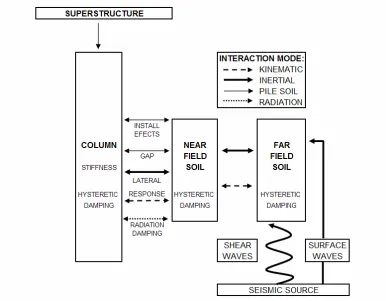
Several interaction modes that exist between a column and the soil around it when subjected
to an earthquake action are depicted in Figure 2.1. The most important modes are kinematic
and inertial. When a pile is driven in soil, it changes the way the soil would have responded
to an earthquake if the pile was not there. This phenomenon is called kinematic interaction
and results in internal forces developing along the pile.
This research focuses on inertial interaction effects. However, it is recognized that the
pile foundation may also experience significant "kinematic" loads that are imposed by the
surrounding soil mass as it deforms relative to the pile during earthquake shaking. Kinematic
loads may not be significant in competent soil profiles that experience relatively small strains
and deformations during shaking. Large kinematic loads can develop, however, due to lateral
spreading of liquefied soils or due to high strain gradients in soft clays, and may be
particularly damaging when the soil stratigraphy consists of alternating stiff and soft layers
along the embedded column length (Wilson D.W. 1998)
The installation procedure also affects the soil-structure interaction, especially under
the influence of axial loads, where driven piles and drilled shafts have different design
methodologies for the same soil. The lateral response, however, seems to be less affected
since the current practice is to use models that were developed and verified for particular soil
types from experiments with both driven piles and drilled shafts (Murchison and O’Neill,
1984). Therefore, in this study no special distinction is made for the design of RC piles and
RC drilled shafts and both are referred as RC columns.
2.2 Models for Soil-Column Interaction
Several techniques have been proposed over time to model piles embedded in soils. These
2.2.1 Continuum analysis: Several variations exist, all using primarily the finite element
method of analysis (Selby A.R. and Arta M.R.,1997) (Brown D, 1990). It is perhaps the more
rigorous approach to model soil-pile systems. Nevertheless the amount of information
required in addition to its complexity and computational cost are maybe justified only for
analysis of special problems.
2.2.2 Equivalent P-y model. This analysis approach is the more commonly used. The soil is
replaced with a series of nonlinear springs closely spaced along the embedded length of the
pile as can be seen in Figure 2.2.a . The force-deformation response of the springs has been
back-calculated from the results of well instrumented lateral load tests of piles in different
soils. In its current state, the method allows for multilayered soils (Geordalis, 1983). There
are several available models for lateral response of soil or P-y models, such as the model for
soft clays under water by Matlock (1970), for stiff clays by Reese (1975) and the integrated
model for clays by O’Neil (1984)
There is software specially developed for the application of this method. Two
commercial packages are MultiPier (BSI, 2000) and LPILE (Ensoft, 2004). MultiPier was
developed in 1994 at the Bridge Software Institute, and some of its features are a built in
interactive pile bent software wizard, models for soil resistance (lateral and axial, single and
group) using methods representing the current state of geotechnical engineering practice and
nonlinear modeling of the structural elements. MultiPier has been used in this research to
P-y models have also been developed to model the dynamic response of soil-column
systems and have been integrated into software packages. OpenSees (McKena F., 2000) was
developed at the Pacific Earthquake Research Center and is an object-oriented framework for
finite element analysis. The program allows the user to perform Nonlinear Time History
Analysis (NTHA) on soil-column models using P-y models for the soil. OpenSees has been
used in this research to perform NTHA on soil-column models.
The P-y equivalent model, although simpler and more practical than the continuum
analysis, is not yet suitable for design purposes since it requires information that may not be
available at the early stages of design, such us the moment-curvature response of the column
section.
2.2.3 Equivalent base spring model. The soil and pile beneath the ground surface is replaced
by coupled translational and rotational springs. The stiffness of the springs must account for
the stiffness of the soil and pile below ground and is obtained on a case by case basis by a
substructuring technique. Although the resultant model is smaller than an equivalent P-y
model, getting the stiffness matrix to model the soil requires significantly more effort making
this procedure less attractive than the P-y method for the analysis of column-soil systems.
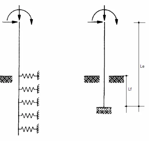
2.2.4 Equivalent cantilever model: the piles are considered fully fixed at some depth below
ground surface and the soil is ignored, as shown in Figure 2.2.b. The embedded length, also
engineer, who can model a single pile as a cantilever and a pile bent as a frame. In both
cases, the piles are fixed at their bases. The result of this simplification is that the structural
computations are straightforward and seem to provide all the required information for design.
That is, for the application of the code-based force based design procedure, the designer can
readily calculate stiffness, fundamental period, and seismic design forces from this model.
Over the last 40 years, several procedures have been proposed for the estimation of Lf
values, such as those proposed by Davisson and Robinson (1965) and Chen (1997). In his
paper, Chen, presents a procedure that yields three Lf values for a pile-soil system: one to
match stiffness, and the others to match moment and buckling capacity. The most often used
Lf equations are those proposed by Davison and Robinson in 1965. These equations have
been incorporated into the AASHTO LRFD Bridge Design Specifications (2004) and their
use is recommended for the assessment of buckling effective length only. For piles in clays,
Lf is evaluated from Equation 2.1, and for piles in sand from Equation 2.2. In both cases, Lf is
measured from the ground level.
In these two equations, Ep and Ipy are the elastic modulus and inertia of the pile, Ec is
the elastic modulus for clays (see Table 2.1 for representative values) and nh is the rate by
which the soil modulus increases with depth in sands (see Table 2.2 for representative
values). Equations 1 and 2 are based on beam on elastic-foundation theory and assume a
long, partially embedded pile laterally loaded in a single uniform layer of either clay or sand.
The coefficients 1.4 in Equation 2.1 and 1.8 in Equation 2.2 are set so the model can
approximately match bending and buckling response simultaneously but will not match
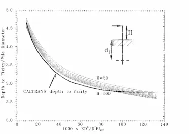
Values of Lf can also be obtained from charts. Figure 2.3 and Figure 2.4 show the
results of a parametric study on columns in sands for pinned and fixed head condition
respectively (Budek A.M. 2000). In this charts the depth to fixity normalized with respect to
column diameter D is plotted against a nondimensional stiffness value, where K is lateral
subgrade modulus of sand, D* is a reference diameter equal to 1.83 m and EIeffis the flexural
stiffness of the column. Figures 2.3 and 2.4 also show the recommendation of Caltrans
(1990) to determine Lf for drilled shafts in sands. The Lf value obtained from Figures 2.3 or
2.4 define the length of an equivalent cantilever that has the same lateral stiffness as the pile
in soil. However, the moment calculated at the base of this cantilever, does not correspond to
the maximum moment in the real column. As an alternative, Lf can be found from the results
of single column lateral nonlinear analysis as proposed by Kowalsky et al. (2005). In this
case, Lf is chosen to match moment in the pile, and the stiffness and buckling capacity are
matched by introducing inertia modifier and length modifier coefficients respectively.
In general, the main drawback of the equivalent cantilever approach is that, for a
multiple soil layer profile, the engineer has to determine an equivalent soil layer of either
sand or clay.
25 . 0 4 . 1 ⎥ ⎦ ⎤ ⎢ ⎣ ⎡ = c py p f E I E
L (Clay) (2.1)
20 . 0 8 . 1 ⎥ ⎦ ⎤ ⎢ ⎣ ⎡ = h py p f n I E
Figure 2.2 Soil-pile models. (a) p-y equivalent model (b) Equivalent cantilever model
Table 2.1. Representative Ec values for clays after Y. Chen (1997)
Clay type su (tsf) Ec (tsf)
Soft 0.25 16.75
Medium 0.47 31.4
Stiff 0.81 54.4
Very stiff 1.47 98.5
Table 2.2. Representative nh values for sands after Y. Chen (1997)
Sand type Saturation
condition nh (tsf/ft)
Moist/dry 30
Submerged 15
Moist/dry 80
Submerged 40
Moist/dry 200
Submerged 100
Loose
Medium
2.3. Nonlinear response of column bents under lateral loads
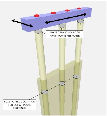
Column bents can be visualized as plane structures. Usually, a line of two or more columns is
attached to a cap-beam. The section, type and length of the columns and the spacing between
them are kept constant within the bent. The in-plane response can be characterized for the
development of maximum moments at the connection with the cap-beam or superstructure. If
the imposed curvature reaches the yield limit, a plastic hinge will develop at this location.
The out-of-plane response includes maximum moments developing at some depth under
ground, and possibly plastic hinges if the imposed curvature reaches the yield limit. The
response in both directions is highly dependent on the above ground length and the flexural
stiffness and strength of the column, and the stiffness and strength of the soil (Figure 2.5).
If the flexural stiffness of the cap-beam is very large compared to the stiffness of the
columns, the in-plane response of the bent can be estimated by looking at the response of a
single column in which, the rotation of the top is restrained (Fixed-head column). The
out-of-plane response however, depends on the type of connection with the superstructure. If the
sub-superstructure connection is rigid, the response is similar to that of a fixed head column.
However, the usual case is to have a pinned connection between the superstructure and the
cap beam and therefore the out-of-plane response can be assessed by analyzing a single pile
or column allowing free rotation at the top (Pinned-head column). Therefore, this research
focuses on the assessment, characterization, and modeling of the nonlinear static and
Figure 2.5 Plastic hinge locations
In 2000, Budek et al investigated the response of drilled shafts in cohesionless soils.
They conducted a series of nonlinear analysis using the equivalent P-y model to study the
force-deformation response, moment pattern, and ductility demand on drilled shafts under a
lateral load applied at the top. In their study, shafts are modeled as a series of nonlinear PLASTIC HINGE LOCATION
FOR OUT-OF-PLANE RESPONSE
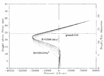
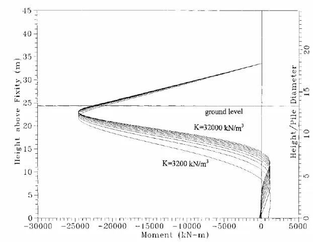
the moment pattern of fixed-head columns when a lateral load has been applied at the top and
the column has reached its ultimate displacement capacity. Figure 2.7 shows the moment
pattern of pinned-head columns. In these figures, K is the lateral subgrade modulus of sand.
Figure 2.7 Moment Patterns at ultimate yield displacement in a pinned-head column in sand (Budek et al, 2000).
Figure 2.8 shows values of plastic hinge length plotted against a nondimensional stiffness
value for pinned head columns. The nondimensional stiffness was described in section 2.2.4.
The plastic hinge length multiplied by the curvature ductility demand yields the total plastic
rotation at the hinge. The under ground plastic hinge lengths are usually larger than the
length for the hinges developed at the top of a fixed head column. In the case of an
underground hinge, the plasticity spreads at both sides of the hinge, and the amount of
spreading is increased by the presence of the soil.
For plastic hinges forming at the top of fixed-head columns, the plastic hinge length
can be calculated from Equation 2.3 (Priestley M.J.N., 1996 ). In this equation L is the
distance from the critical section to the point of inflection in meters, fy is the yield strength in
MPa, and dblis the longitudinal bar diameter in meters.
bl y
p L f d
l =0.08 +0.022 (2.3)
The first term in Equation 2.3 represents the spread of plasticity resulting from variation in
curvature with distance from the critical section, and assumes a linear variation in moment
with distance. The second term represents the increase in effective plastic hinge length
2.4 Ductility Models
In 2002, Chai Y.H. proposed an analytic model to assess the local ductility demand of a
yielding pile using the equivalent cantilever model shown in Figure 2.9. This model is
applicable to single column bents and uses a point of fixity that matches the stiffness of the
soil-column system. The depth to the point at which the maximum underground moment
occurs is determined separately. The total top displacement is then found as the sum of the
elastic displacement ∆y (Equation 2.4) plus the plastic displacement ∆p (Equation 2.5).
EI L L
V f a
y
3 )
( + 3
=
∆ (2.4)
) ( m a
p
p = L +L
∆ θ (2.5)
) ( u y
p
p L φ φ
θ = − (2.6)
In Equations 2.4-2.5, ∆y is the yield elastic displacement, V is the yield lateral force, Lf is the
depth to fixity, La is the height of the column, Lm is the depth to the point of maximum
moment, EI is the product of the elastic modulus and inertia of the column, θp is the plastic
rotation at the plastic hinge, Lp is the plastic hinge length and φu and φy are the ultimate and
yield curvatures. This model allows the estimation of lateral strength and the assessment of
the local curvature ductility demand in the column for any value of displacement ductility
demand at the top of the pile. The elastic stiffness used in this model comes from the elastic
Winkler model developed by Poulos and Davis (1980).
2.5 Special effects of earthquake loading.
So far we have covered the nonlinear response of column-soil systems under the effect of
lateral load acting at the column top. During an earthquake however, the cyclic nature of the
excitation can cause the formation of a gap between the soil and the column. This is due to
nonlinear nature of the soil response and to the fact that the soil does not resist tension. As a
result of that, the stiffness of the column system is reduced and continually degraded during
Figure 2.9/a shows the results of a lateral cyclic load test performed by Matlock in
1970. In this test a pipe pile was push laterally while embedded in soft clay. Figure 2.9/b.
shows the results of a simulation performed using OpenSees with the pysimple1 element
(Boulanger, R.W., 2003).
Figure 2.9 a)Result of Matlock’s experiment in soft clay b) Result of simulation with pysimple1 element
Figure 2.9 show that even though the pysimple1 element in OpenSees does not model
strength degradation, it can reasonably capture the force deformation response of pile-soil
systems in soft clay. The pysimple1 element in OpenSees has been further verified with the
results of centrifuge experiments (Boulanger et al, 1999).
2.6 Review of the current design practice
1. Obtain an equivalent cantilever model for the pile-soil system. The depth to fixity is
chosen from design charts, to match the stiffness of the pile-soil system.
2. Build a bridge model. Once each pile and the surrounding soil have been replaced by
a single frame element, a complete model of the bridge is built by adding the other
pile and superstructure elements. Boundary conditions, mass, section properties, and
loads are then assigned to the model.
3. A modal analysis is performed. The fundamental period is found.
4. The design base shear is found from the appropriate design spectra, using the mass,
the period and the force reduction factor R. ATC 40 (1996) considers piles/drilled
shafts, as structures of limited ductility and recommends R equal 4. AASHTTO
LRFD Bridge Design Specifications (2004) recommend values of 1.5 for bents
classified as critical, 3.5 for essential bents and 5 for other bents.
5. Then an elastic analysis is performed and element internal forces are found for
design.
6. The design of the column bent is then performed using special purpose software such
as MultiPier (BSI, 2000) or L-pile (Ensoft, 2004). The use of these special codes
allows for a more precise determination of the moments that develop along the pile,
2.7 Direct Displacement Based Design (DDBD)
DDBD works by inverting the traditional seismic design process. For a specified target
displacement and earthquake intensity, the method yields the required stiffness and strength.
DDBD has been successfully implemented for the design of bridge RC piers (Kowalsky M.J
et al 1995) and for RC frames (Priestley M.J.N and Kowalsky M.J., 2000). The procedure is
based on the following arguments:
- The yield curvature/displacement can be estimated from the geometry of the section
- A nonlinear system can be substituted by a single degree of freedom linear system
that has an effective mass, effective period and equivalent viscous damping.
To apply DDBD for the design of column bents, the following procedure could be
followed:
• Gather basic information such as: Length above ground, diameter of the column,
weight acting on the bent, soil type and strength.
• Establish the Target Displacement and Displacement Ductility demand.
• Determine the equivalent viscous damping. Due to the soil-structure interaction, the
equivalent viscous damping is a combination of viscous damping, hysteretic damping
in the column and hysteretic damping in the soil.
The procedure presented above is similar to what has been proposed for bridge piers
(Kowalsky M.J. et al, 1995). However, piers that are supported on rigid pile caps at soil level
are likely to develop plastic hinges above ground only. So, the equivalent damping is a
combination of viscous damping and hysteretic damping in the column only (Dwairi H.M.,
2005).
This section concludes the literature review, in which the most relevant information
about the analysis and design of column bents as well as the implementation of DDBD was
summarized. Next, Chapter 3 presents the results of several static and dynamic nonlinear
analyses conducted to demonstrate the performance of the P-y equivalent models, and also
3. MODELING THE SOIL-PILE INTERACTION
3.1 Soil Properties
Throughout this study, the soil used in the analyses has the properties denoted in Table 3.1
for clay and Table 3.2 for sand. The characterization of clay has been done in terms of shear
strength su, then strains at 50% and 100% of the ultimate shear strength, ε50 and ε100, and
total unit weight w. The characterization of sand has been done in terms of friction angle φ,
lateral subgrade modulus k, and unit weight w.
Table 3.1 Properties of Clay Soils
CLAYS Su (Kpa) e50 e100 w (kN/m3)
Clay-20 20 0.02 0.06 16
Clay-40 40 0.015 0.06 17
Table 3.2 Properties of Sand Soils
SANDS φ k (kN/m3) w (kN/m3)
Sand-30 30 5500 16.7
Sand-34 34 16600 17.6
Sand-37 37 33200 18.5
The properties of the soils were taken from Reese and Impe (2001) as recommended values
to use with Matlock’s (1970) P-y model for soft clays and the Reese’s (1974) P-y model for
3.2 Group Effects
When a group of piles is pushed laterally, is it possible that the lateral stiffness of the system
be less than the sum of the stiffness of individual soil-pile systems, this is due to the
pile-soil-pile interaction that occurs when the separation between pile-soil-piles is small. For pile-soil-pile or column
bent design, the group effects vanish for in-line piles at spacing equal to three diameters or
more (Schmidt, 1985). In column bents, the spacing between columns is generally larger
than three diameters of the column. Therefore the group effects were not included in this
study.
3.3 Nonlinear Static Response
This section shows the results of five lateral nonlinear static analyses of a 0.90m diameter RC
column embedded in soil. The column is 5.40m high and is embedded 27m. Two analyses
were performed for fixed and pinned conditions with the column embedded in clay and two
analyses were performed for fixed and pinned conditions with the column embedded in sand.
Both MultiPier and OpenSees were used for each analysis. The primary purpose of these
analyses was to gain experience in the use and to verify the capabilities of OpenSees.
In both MultiPier and OpenSees the column is modeled as a series of column
elements and the soil is modeled as nonlinear springs attached to the connections between the
column elements. Both soil and column elements are modeled using nonlinear formulations.
programs are accounting for a similar section response for the column. This was done by
conducting analyses with both programs in which an increasing moment was applied at the
end of a cantilever column element with length equal to one. The rotation of the free node is
the curvature that corresponds to the applied moment.
Figure 3.1 shows the moment curvature response obtained by both programs.
MultiPier requires the user to input the material properties, reinforcement, and geometry, and
defines a fiber section. Thus the response shown in Figure 3.1 is nonlinear and smooth. In
OpenSees the user can choose the type of formulation to use for the column elements, the
sections can be defined either as fiber sections or the user can input a section response model.
For these analyses, once the section response was found by MultiPier, it was converted into a
bilinear model and entered in OpenSees.
M_C RESPONSE 0.90m DIAMETER RC COLUMN
0 500 1000 1500 2000 2500 3000
0 0.005 0.01 0.015 0.02 0.025 0.03 0.035 0.04
CURVATURE (1/m)
MOME
N
T
(
k
N
-m)
BILINEAR MPier
Clay was modeled in MultiPier using the built-in P-y model for soft clays under water
proposed by Matlock (1970). In OpenSees the soil is modeled using the pysimple1 developed
by Boulanger (2003) element with parameters recommended to match the same clay model
used in MultiPier. The sand was modeled in MultiPier using the built-in p-y model for sand
proposed by Reese et al (1974). In OpenSees the soil is modeled using the pysimple1 element
and the P-y model for sands recommended by the American Petroleum Institute (API, 1987)
which is built-in OpenSees and is similar to the model used in MultiPier.
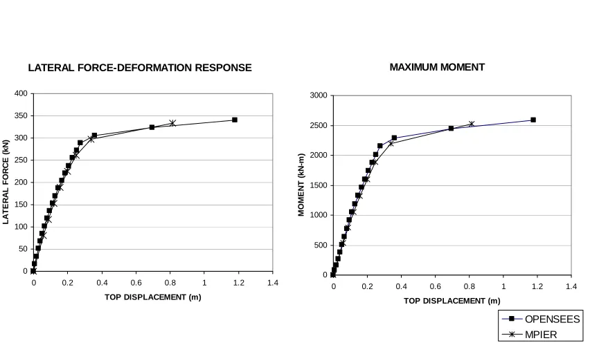
Figures 3.2 and 3.3 show the lateral force deformation response of the RC column in
clay for the fixed head and pinned head conditions. Figures 3.4 and 3.5 show the lateral force
deformation response of the RC column in sand for the fixed head and pinned head
conditions. The results from each program agree with each other so it was concluded that
the modeling techniques used in OpenSees are appropriate. And therefore OpenSees can be
used as an analysis tool.
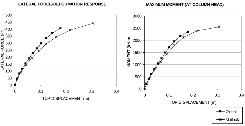
Finally another nonlinear analysis was performed only with MultiPier to compare the
lateral response of the RC column when the soil is modeled using the model for soft clays
(Matlock 1970) and the integrated model for clays proposed by O’Neill (1984). O’Neill’s
model was developed to encompass soft and stiff clays. As it can be observed in Figure 3.6
Matlock’s model is lees stiff than the O’Neill’s.
Although it would be beneficial to use O’Neill’s integrated model since it encompass
soft and stiff clays, this is not possible because OpenSees only models Clay using Matlock’s
different. As a result of this, the present study is constrained to the implementation of DDBD
for column bents in sand and soft clay only.
Figure 3.2 Lateral response of a fixed head RC column in clay
Figure 3.3 Lateral response of a pinned head RC column in clay
LATERAL FORCE-DEFORMATION RESPONSE
0 50 100 150 200 250 300 350 400 450 500
0 0.1 0.2 0.3 0.4
TOP DISPLACEMENT (m)
LAT E R A L FO R C E ( k N )
MAXIMUM MOMENT (AT COLUMN HEAD)
0 500 1000 1500 2000 2500 3000
0 0.1 0.2 0.3 0.4
TOP DISPLACEMENT (m)
MOME N T ( k N -m OPENSEES MPIER
LATERAL FORCE-DEFORMATION RESPONSE
0 50 100 150 200 250 300 350
0 0.2 0.4 0.6 0.8
TOP DISPLACEMENT (m)
LA TE R A L F O R C E ( k N ) MAXIMUM MOMENT 0 500 1000 1500 2000 2500
0 0.2 0.4 0.6 0.8
TOP DISPLACEMENT (m)
Figure 3.4 Lateral response of a fixed head RC column in sand
Figure 3.5 Lateral response of a pinned head RC column in sand
LATERAL FORCE-DEFORMATION RESPONSE
0 50 100 150 200 250 300 350 400
0 0.2 0.4 0.6 0.8 1 1.2 1.4 TOP DISPLACEMENT (m)
L A TE R A L F O R C E ( k N ) MAXIMUM MOMENT 0 500 1000 1500 2000 2500 3000
0 0.2 0.4 0.6 0.8 1 1.2 1.4 TOP DISPLACEMENT (m)
M O M E NT ( k N-m ) OPENSEES MPIER
LATERAL FORCE-DEFORMATION RESPONSE
0 100 200 300 400 500 600 700
0 0.05 0.1 0.15 0.2 0.25 0.3 0.35
TOP DISPLACEMENT (m)
L A T E RAL FO RCE (kN)
MAXIMUM MOMENT (AT COLUMN HEAD)
0 500 1000 1500 2000 2500 3000
0 0.05 0.1 0.15 0.2 0.25 0.3 0.35
TOP DISPLACEMENT (m)
MO
ME
NT (kN-m)
Figure 3.6 Response of a fixed head RC column with Matlock and O’Neill models for clays.
3.4 Nonlinear Time History Analysis (NLTH) using OpenSees
In this section, the results of two NLTH analyses are presented. The analyses consisted of the
application of an earthquake acceleration record to a fixed head RC column with the soft clay
model. The RC column is 0.60m in diameter and 3.6m high. Figure 3.7 shows two cycles of
the moment curvature response of the column. This was achieved by using the Hysteretic
Bilinear (McKenna F. et al, 2004) model built-in to OpenSees with pinching coefficients of
0.7 for curvature and 0.2 for moment. The soil was modeled using the pysimple1 elements
described previously with the referenced parameters to match Matlock’s p-y model for soft
clays.
LATERAL FORCE-DEFORMATION RESPONSE
0 50 100 150 200 250 300 350 400 450 500
0 0.1 0.2 0.3 0.4
TOP DISPLACEMENT (m)
LA TE R A L FO R C E ( k N )
MAXIMUM MOMENT (AT COLUMN HEAD)
0 500 1000 1500 2000 2500 3000
0 0.1 0.2 0.3 0.4
TOP DISPLACEMENT (m)
In both analyses the acceleration record shown in Figure 3.8 was applied without
amplification first and then with an amplification factor of 6 for the second analysis. This
accelerogram was measured during the Imperial Valley earthquake in 1979 at the Station
5053.
Cyclic Moment-Curavture Response
-1000 -800 -600 -400 -200 0 200 400 600 800 1000
-0.1 -0.09 -0.08 -0.07 -0.06 -0.05 -0.04 -0.03 -0.02 -0.01 0 0.01 0.02 0.03 0.04 0.05 0.06 0.07 0.08 0.09 0.1
Cuvature (1/m) Mo m e n t (k N )
Figure 3.7 Hysteretic moment curvature response of a 0.60m diameter RC column
Acceleration Record -300 -200 -100 0 100 200 300
0 5 10 15 20 25 30 35
Time (s) A ccel er at ion ( c m /s^ 2 )
Figure 3. 9 a) Displacement history b) Shear history c) Moment history of a 0.6 m diameter RC column Displacement History -0.50 -0.40 -0.30 -0.20 -0.10 0.00 0.10 0.20 0.30 0.40 0.50
0 5 10 15 20 25 30 35
D ispl acem en t at co lu m n head ( m ) Amp6 Amp1 Shear History -300 -200 -100 0 100 200 300
0 5 10 15 20 25 30 35
S h ear a t co lu m n head ( k N ) Amp6 Amp1 Moment History -1000 -800 -600 -400 -200 0 200 400 600 800 1000
0 5 10 15 20 25 30 35
The results in terms of displacement history, shear force history and moment history are
shown in Figure 3.9 for both amplification values. The hysteretic force-deformation
response for both analyses is also shown in Figure 3.10. The small loops in Figure 3.10.b
correspond to the energy dissipated by the hysteretic behavior of the soil only, since at this
level of demand the column has remained elastic. The big loops in Figure 3.10.a represent the
energy that has been dissipated by the soil and the column after both have yielded.
In general the results of these analyses demonstrate the capabilities of OpenSees to
simulate the behavior of column-soil systems. The OpenSees code used for these analyses
can be found in appendix 1.
a) b)
Figure 3.10 Hysteretic force deformation response of a 0.6m D RC column in clay Force-Deformation Response Amp6
-300 -200 -100 0 100 200 300
-0.50 -0.40 -0.30 -0.20 -0.10 0.00 0.10 0.20 0.30 0.40 0.50
Lateral Displacement (m)
S h ear at c o lu m n h e ad ( k N )
Force-Deformation Response Amp1
-300 -200 -100 0 100 200 300
-0.50 -0.40 -0.30 -0.20 -0.10 0.00 0.10 0.20 0.30 0.40 0.50
4. DISPLACEMENT AND DUCTILITY MODELS
4.1 Definition of the equivalent model
As it was discussed in section 2.7, the implementation of DDBD for column bents requires
the development of a model to predict the target displacement and ductility demand of
columns embedded in soil. This model should account for both pinned and fixed head
conditions, different types of soil, and different column heights and diameters. The location
of plastic hinges must also be determined to assess the plastic deformation.
In section 2.2 several modeling approaches were described and discussed. It was
explained that the equivalent cantilever models are perhaps the most promising for the
implementation of DDBD since the formulation is simple and, if defined appropriately, can
produce all the parameters required for the computation of seismic forces.
In this study, a variation of the equivalent cantilever model proposed by Chai (2002)
(Figure 2.9) is presented. The idea behind this new model is to have a column, fixed at the
base, with a length such that the base of the column coincides with the location of the
underground hinge in the real column-soil system. In this manner the plastic displacement at
the top of the equivalent and the soil-column system are the same (Figure 4.1). Also, the
that the force-deformation response of the system is bilinear and that the plastic hinge length
varies linearly with the displacement ductility demand. (Figure 4.2)
In most column bents, each column exhibits free head displacement when pushed out
of the bent’s plane and fixed head displacement when pushed along the plane of the bent, this
is due to the flexibility of the super-to-substructure connection and to the high stiffness of
the cap beam. It has been observed that the depth to the point of maximum moment and
consequently the location of the underground plastic hinge goes deeper if the head restraints
are changed from pinned to fixed (Budek A.M. et al, 2000). Thus, two lengths could be
specified for the same column in order to match in plane and out of plane behavior.
Nevertheless, it has also been observed that in a fixed head column the plastic displacement
caused by an underground hinge is negligible when compared to the plastic displacement
caused by the hinge at the column’s top. Therefore, the location of the underground hinge is
not very important for fixed head columns, and the length used for the pinned head case
could be used for the analysis in both directions.
The proposed model is aimed to predict the target displacement (∆D) and the
displacement ductility (UD). To define the equivalent model, the following parameters must
be determined (Figure 4.1):
• The equivalent length (Le): The length from the cap beam to the expected location of
the underground plastic hinge.
• A stiffness coefficient (α): A correction factor used to match the yield displacements
• An initial plastic hinge length (Lpo) and the slope (Slp): Parameters that define a linear
variation of plastic hinge length with respect to the displacement ductility (UD)
demand on the system (Figure 4.2/b). The plastic hinge length (Lp) relates plastic
rotation to plastic curvature in a plastic hinge. And UD is the ratio between ∆D and the
Displacement Ductility Top Displacement L a tera l F orc e Pl as ti c Hi n g e L en gt h (L p )
Yield Displacement (∆y)
Lpo
Plastic Displacement (∆p)
SLp
1
Target Displacement (∆D) Target Ductility (UD)
Figure 4.2 a) Bilinear force deformation response b) Plastic hinge length as a linear function of ductility
Charts with values for Le , α , Lpo and Slp are shown in Section 4.1.2 for different types of
soils and for different ratios of above ground height to column diameter. These proposed
values, resulted from the parametric study described in Section 4.1 that looked at the
response of single soil-column systems under lateral loads.
Once Le and α are determined, the yield displacement ∆y is found from Equation 4.1
and 4.2 for the pinned head and fixed head columns respectively. In these equations φy is the
yield curvature for the column section that can be calculated using Equation 4.3 (Kowalsky,
2000) where εy is the yield strain for the reinforcing steel and D is the diameter of the
column. 3 2 e y y L φ α =
6 2 e y y L φ α =
∆ (Fixed head columns) (4.2)
D
y y
ε
φ =2.45 (4.3)
In the proposed model, the target displacement ∆D is defined as:
p y
D =∆ +∆
∆ (4.4)
Where ∆y is the yield displacement and ∆p is the plastic displacement of the column equal to:
e p p
p =φ L L
∆ (4.5)
The plastic curvature φp is related to the curvature ductility µφas:
y
p µ φ
φ =( φ −1) (4.6)
If Lp is defined as a linear function of the displacement ductility UD (Figure 4.2.b);
Lp = Slp UD + Lpo (4.7)
And if equations 4.6 and 4.5 are replaced into Equation 4.4, an equation that relates plastic
curvature φp to displacement ductility UD is found:
p e Lp y p e po y D L S L L U φ φ − ∆ + ∆
= (4.8)
Equation 4.8 can also be written in terms of curvature ductility µφ:
y e Lp y y e po y D L S L L U φ µ φ µ φ φ ) 1 ( ) 1 ( − − ∆ − + ∆
= (4.9)
the stiffness of the system. For perfect elasto-plastic systems, Lpo is constant, therefore SLp
equals 0 and Equation 4.9 yields a straight line (Figure 4.3). When SLp is greater that 0 as for
elasto-plastic systems with a non-zero second stiffness, the relation between UD and µφ is
nonlinear.
Figure 4.3. Curvature vs. Displacement ductility for systems with bilinear force deformation response
Equation 4.9 is fundamental for the application of DDBD since it allows the calculation of
UD from a chosen damaged based value of µφ. The value of UD is used to calculate the
equivalent viscous damping for the system (Chapter 5) and to calculate the target
displacement, ∆D, as follows:
∆D = (UD −1 ) ∆y (4.10)
Displacement Ductility
Cu
rvat
u
re Du
ct
il
it
y
1 1
Slp>0
An evaluation of equation 4.9 is presented in Section 4.3 based on the results of detailed
nonlinear lateral static analyses.
4.2 Parametric study.
This study aims to provide the parameters required to calculate the target displacement and
ductility demand using the equivalent model described in the previous section. A series of
parametric analyses have been performed to find trends to predict the location of the
underground plastic hinge, yield displacement and plastic hinge length in soil-column
systems.
4.2.1 Procedure
Curvature
M
om
en
t
φy
My
1
EIcr
rEIcr
The study consisted in performing a series of nonlinear static analyses. In each analysis an
incremental lateral load was applied at the top of a RC column embedded in sand or clay.
The column-soil system was modeled using a bilinear moment curvature response for the
column elements and a nonlinear P-y model for the soil springs. The length of the column
elements was set to one quarter of the diameter of the column. Figure 4.4 depicts the moment
curvature response assigned to the column elements. E is the elastic modulus of concrete.
The cracked moment of inertia (Icr) of the column’s section was taken as 50% of the gross
moment of inertia to account for cracking. This reduction factor was taken from
recommendations of Caltrans (2004) for concrete columns with 2% reinforcement ratio and
subjected to an axial load equivalent to 20% the capacity of the section. The yield curvature
(φy) is obtained from Equation 4.3. and the yield moment (My) from Equation 4.11. The
curvature ductility demand (µφ) at any point after yield can be also computed with equation
4.12 where the maximum moment in the column is M.
y
y EI
M =0.5 φ (4.11)
y y y
rEI M M
φ φ
µφ +
−
= (4.12)
The general configuration of the soil-column model was varied for each analysis and
included: pinned or fixed head condition for the column, diameters of the column ranging
the displacement at the column tip was negligible. The properties of the soils that were used
are summarized in Table 4.1. Table 4.2 shows the parametric matrix used for the analyses.
Table 4. 1. Definition of soil parameters
CLAYS Su (Kpa) e50 w (kN/m3) P-y model
Clay-20 20 0.02 16 Matlock
Clay-40 40 0.015 17 Matlock
SANDS φ k (kN/m3) w (kN/m3) P-y model
Sand-30 30 5500 16.7 API
Sand-34 34 16600 17.6 API
Sand-37 37 33200 18.5 API
Table 4. 2. Parametric Matrix for Pushover Analyses
HEAD D (m) La/D Soils
PINNED 0.3 2 Clay-20
FIXED 0.6 4 Clay-40
0.9 6 Sand-30
1.2 8 Sand-34
1.5 10 Sand-37
1.8 2.4
Number of combinations: 350
The program OpenSees was used to perform the analyses. In each analysis the lateral load
was applied with small increments until the analysis failed to converge. For each increment
in lateral load, the following parameters were recorded: top displacement, applied force at
elements below ground in a depth of ten pile diameters. Then, using post-processing, the
following parameters were found for each system:
• Yield displacement: as the top displacement at which the maximum moment along
the column reached the value of yield moment calculated from Equation 4.11
• The location of the underground point of maximum moment and the location of the
point of inflection for fixed-head columns only: by looking at the moment pattern
along the column.
• The curvature ductility demand at each point after yield: from Equation 4.12
• The plastic hinge length: from Equation 4.13 where ∆ and φ are the top displacement
and hinge curvature at the point in the force-deformation response at which Lp is
being calculated.
(
y)
e y p
L L
φ φ−
∆ − ∆
= (4.13)
4.1.2 Results
By performing the analyses it was found that, for each soil type, there is a linear fit between
the equivalent length normalized by the diameter of the column (Le/D) and the normalized
for sands within the range of soil parameters considered. Figure 4.5 shows the data for
columns in sand while Figure 4.6 shows the data for columns in clay. Table 4.3 presents the
best fit equations with the corresponding R-squared values.
The correlations for Le are good, better for clay than for sand. These correlations are
very important since allow the assessment of the underground plastic hinge location very
easily based on information known at the early stages of design.
A trend was also identified the parameter α . Figures 4.7 and 4.8 show the data for
fixed head columns in clay and sand respectively, while Figures 4.9 and 4.10 show the data
for pinned head columns in clay and sand respectively. The trends that were identified are
independent for each soil type and are summarized in Table 4.4 for fixed head columns and
in Table 4.5 for pinned head tables.
4 6 8 10 12 14 16
0 2 4 6 8 10 12
La/D
Le/
D
Sand-30 Sand-34 Sand-37 Trend Sand-30 Trend Sand-37
6 7 8 9 10 11 12 13 14
0 2 4 6 8 10 12
La/D
Le/
D
Clay-20 Clay-40 Trend Clay-20 Trend Clay-40
Figure 4.6. Le/D as a function of La/D for Columns in Clay
Table 4.3. Trends for Le/D for Columns in soft clay and sand
SOIL TYPE TREND R-squared
Clay-20 ⎟
⎠ ⎞ ⎜ ⎝ ⎛ + = D L D
Le a
69 . 0 38 . 6 0.98
Clay-40 ⎟
⎠ ⎞ ⎜ ⎝ ⎛ + = D L D
Le a
71 . 0 96 . 4 0.99
Sand-30 ⎟
⎠ ⎞ ⎜ ⎝ ⎛ + = D L D
Le a
82 . 0 39 . 4 0.84
Sand-37 ⎟
⎠ ⎞ ⎜ ⎝ ⎛ + = D L D
Le a
1.7 1.9 2.1 2.3 2.5 2.7
0 2 4 6 8 10 12
La/D
α
Clay-20 Clay-40 Trend Clay-20 Trend Clay-40
Figure 4.7. α as a function of La/D for Fixed Head Columns in Clay
1.3 1.4 1.5 1.6 1.7 1.8 1.9
0 2 4 6 8 10 12
La/D
α
Sand-30 Sand-34 Sand-37 Trend Sand-30 Trend Sand-37
y
2.5 2.7 2.9 3.1 3.3 3.5 3.7 3.9 4.1 4.3 4.5 4.7 4.9
0 2 4 6 8 10 12
La/D
α
Clay-20 Clay-40 Trend Clay-20 Trend Clay-40
Figure 4.9. α as a function of La/D for Pinned Head Columns in Clay
1.5 1.7 1.9 2.1 2.3 2.5 2.7 2.9 3.1 3.3 3.5
0 2 4 6 8 10 12
La/D
α
Sand-30 Sand-34 Sand-37 Trend Sand-30 Trend Sand-37
Table 4.4. Trends for α for fixed head Columns in sand and soft clay
SOIL TYPE TREND R-squared
Clay-20 ⎟
⎠ ⎞ ⎜ ⎝ ⎛ − = D La ln 38 . 0 84 . 2 α 0.90
Clay-40 ⎟
⎠ ⎞ ⎜ ⎝ ⎛ − = D La ln 33 . 0 68 . 2 α 0.90
Sand-30 ⎟
⎠ ⎞ ⎜ ⎝ ⎛ − = D La ln 16 . 0 88 . 1 α 0.72
Sand-37 ⎟
⎠ ⎞ ⎜ ⎝ ⎛ − = D La ln 18 . 0 86 . 1 α 0.88
Table 4.5. Trends for α for Pinned Head Columns in sand and soft clay
SOIL TYPE TREND R-squared
Clay-20 ⎟
⎠ ⎞ ⎜ ⎝ ⎛ − = D La ln 09 . 1 52 . 5 α 0.95
Clay-40 ⎟
⎠ ⎞ ⎜ ⎝ ⎛ − = D La ln 08 . 1 30 . 5 α 0.96
Sand-30 ⎟
⎠ ⎞ ⎜ ⎝ ⎛ − = D La ln 67 . 0 56 . 3 α 0.95
Sand-37 ⎟
The parameter α is larger for pinned head columns, and it is also larger for clays. The
parameter α is the ratio between the yield displacement of a cantilever column with length Le
and the yield displacement of the same column embedded in soil. The two yield
displacements are different since the rotation at the underground point of maximum moment
is not cero for the column-soil system and because the area inside the curvature diagram of
the column-soil system from the point of maximum moment up is bigger than the
corresponding for the cantilever column. Therefore it can be expected a higher value of
α for the pinned head columns, since the underground rotation at the point of maximum
moment is less that the corresponding for a fixed head column. α is also higher for clay
because sands increase in strength with depth where as clays do not, therefore less rotation
bellow the point of maximum moment is expected for sands.
The post yielding stage was also examined and linear trends were found for Slp . The
trends are presented for each of the soil type and head restraint condition. However, no well
defined trend was found for Lpo and due to the small scatter only average values are shown.
The data has been plot in Figures 4.11 and 4.12 for fixed head columns in clay and sand
respectively and in Figures 4.13 and 4.14 for pinned head columns in clay and sand
respectively. Equations for the trends and average values of Lpo can be found in Table 4.6 and
0.1 0.12 0.14 0.16 0.18 0.2 0.22 0.24 0.26
0 2 4 6 8 10 12
La/D
Slp
/D
Clay-20 Clay-40 Trend Clay-20 Trend Clay-40
Figure 4.11. Slp/D as a function of La/D for Fixed Head Columns in Clay
0.05 0.07 0.09 0.11 0.13 0.15 0.17 0.19 0.21 0.23
0 2 4 6 8 10 12
La/D
Slp
/D
Sand-30 Sand-37 Trend Sand-30 Trend Sand-37
0.3 0.35 0.4 0.45 0.5 0.55 0.6 0.65 0.7
0 2 4 6 8 10 12
La/D
Sl
p
/D
Clay-20 Clay 40 Trend Clay-20 Trend Clay-40
Figure 4.13. Slp/D as a function of La/D for Free Head Columns in Clay
0.1 0.12 0.14 0.16 0.18 0.2 0.22 0.24 0.26 0.28
0 2 4 6 8 10 12
La/D
Sl
p
/D
Sand-30 Sand-37 Trend Sand-30 Trend Sand-37
Table 4.6. Trends for Slp/D for Fixed Head Columns in soft clay and sand
SOIL TYPE TREND R-squared Average Lpo/D
Clay-20 =0.0042 +0.18
D L D
Slp a
0.65 0.08
Clay-40 =0.0076 +0.13
D L D
Slp a
0.87 0.08
Sand-30 =0.013 +0.064
D L D
Slp a
0.79 0.07
Sand-37 =0.015 +0.040
D L D
Slp a
0.81 0.07
Table 4.7. Trends for Slp/D for Pinned Head Columns in soft clay and sand
SOIL TYPE TREND R-squared Average Lpo/D
Clay-20 =0.0053 +0.55
D L D
Slp a
0.06 1.9
Clay-40 =0.0053 +0.41
D L D
Slp a
0.31 1.9
Sand-30 =0.0102 +0.14
D L D
Slp a
0.82 1.5
Sand-37 =0.0116 +0.10
D L D
Slp a
The trends that were found for Lpo and Slp define the plastic hinge length so the equivalent
model matches the theoretic plastic displacement of the nonlinear soil-column model as it
will be shown in the next section. In the literature review were described a few existing
models for underground plastic hinge length (Budek et al, 2000) (Chai et al, 2002). In these
models the plastic hinge length is considered constant with respect to the displacement
ductility. This assumption is theoretical valid for a perfect elastic plastic system, and might
be appropriate for columns embedded in stiff soils where the force deformation response
follows that pattern.
The application of DDBD as described in Section 2.7 yields a design base shear (V) for a
column-soil system. To design the column section however, it is necessary to translate V into
a design moment for the column (Mu). Figure 4.15 shows a force diagram for a pinned head
column. The applied force V at the top of the column, is resisted by the soil from the ground
down to the point of maximum moment. The maximum moment in the pile Mu is given by
Equation 4.14.
)) (
( e e a
u V L L L
M = −β − (4.14)
The coefficient β has been calculated from the results of the parametric study as shown in the
following table:
Le
La
Mu
V
β(Le-La)
Figure 4.15 Force diagram for a pinned head column.
Table 4.8 β values for calculating Mu in pinned-head columns
SOIL β Standard
Deviation σ β-2σ
CLAY 0.40 0.03 0.33
SAND 0.32 0.03 0.26
To calculate the maximum moment in fixed head columns once the base shear V is known, it
is necessary to know the length from the top of the column to the inflection point (Li), then
Mu can be calculated from Equation 4.15. Values of Li have been found from the parametric
analysis and are summarized in Table 4.9
i
u VL
Table 4.9 Li / Le for calculating Mu in fixed-head columns
SOIL Li/Le
Standard Deviation
σ
Li/Le+2σ
CLAY 0.59 0.02 0.63
SAND 0.52 0.02 0.56
4.3 Evaluation of the proposed models
The applicability of the proposed models is limited to the range of the parameters used in the
parametric study. Verification analyses were conducted by comparing with results of
nonlinear lateral static analyses. Each of these nonlinear analyses involved the application of
an incremental static load at the top of a 0.9 m diameter RC column with 5.4 m in height
above ground (Table 4.10). The column was considered embedded in four different soil types
and the analyses were performed with pinned and fixed head conditions.
Table 4.10. Parametric matrix for evaluation of kinematic model
Analysis No Height (m) Diameter (m) Head
Restraints EI (kN.m
2
) Soil
1 5.4 0.9 Fixed 437548 Clay-20
2 5.4 0.9 Fixed 437548 Clay-40
3 5.4 0.9 Fixed 437548 Sand-30
4 5.4 0.9 Fixed 437548 Sand-37
5 5.4 0.9 Pinned 437548 Clay-20
6 5.4 0.9 Pinned 437548 Clay-40
7 5.4 0.9 Pinned 437548 Sand-30
4.2.1 Results of Nonlinear Analyses
The analyses were performed using OpenSees with models of similar characteristics
to those described in Section 3.2. The force deformation response for analyses 1 to 4 is
presented in Figure 4.16/a and for analyses 5 to 8 in Figure 4.16/b
Figure 4.16 makes evident the higher strength and stiffness of the fixed head
columns. Figure 4.16 also shows that the yield displacement of the system depends on the
strength and stiffness of the soil. With the soil models and strength parameters used in this
study, Clay-20 seems to provide the least stiffness while Sand-37 the biggest. The response
of the fixed head columns noticeably changes in stiffness, these corresponds to the formation
of the top hinge and then the underground hinge. It can also be noticed that the hinges
develop at closer lateral displacement as the stiffness of the soil increases. For the fixed head
cases, the yield displacement is taken as the lateral displacement that causes the development
of the top hinge.
The location of the underground point of maximum moment is presented for the fixed
head cases in Figure 4.17/a and for the pinned head cases in Figure 4.17/b. As it was
explained in Section 4.1, the location of the maximum underground moment is slightly
deeper for fixed head columns. In general the point of maximum moment tends to go deeper
as the lateral load increases, then becomes stable after yielding of the column.
Figure 4.18 shows the variation of plastic hinge length with respect to the
agreed that the depth to maximum moment for pinned head columns will be used also for the
fixed head case.
Figure 4.16. Force-Deformation response a) Fixed Head b) Pinned Head
The relation between curvature ductility demand and displacement ductility demand for the
Force-Deformation Response. Fixed Head Columns
0 100 200 300 400 500 600 700 800 900 1000
0 0.1 0.2 0.3 0.4 0.5 0.6
Top Displacement (m)
L a te ra l F o rc e (k N )
Force-Deformation Response. Pinned Head Columns
0 50 100 150 200 250 300 350 400
0 0.1 0.2 0.3 0.4 0.5 0.6
Top Displacement (m)
L a te ra l F o rc e (k N )
the pinned head cases. It is observed that the relation between curvature and displacement
ductility does not depend much on the soil type.
Location of Point of Maximum Moment. Fixed Head Columns
0 2 4 6 8 10 12 14
0 0.1 0.2 0.3 0.4 0.5 0.6
Top Displacement (m)
L eng th f ro m C o lu m n t op (m )
Location of Point of Maximun Moment. Pinned Head Columns
0 2 4 6 8 10 12 14
0 0.1 0.2 0.3 0.4 0.5 0.6
Top Displacement (m)
Le ngt h f rom C o lu m n t o p ( m )
Figure 4.18. Plastic hinge length a) Fixed Head b) Pinned Head
Plastic Hinge Length for Pinned Head Columns
0 1 2 3 4 5 6
1 1.5 2 2.5 3 3.5 4
Displacement Ductility
P
last
ic H
in
ge L
engt
h
(
m
)
Clay-40 Sand-30 Sand-37 Clay-20
Plastic Hinge Length for Fixed Head Columns
0 0.1 0.2 0.3 0.4 0.5 0.6 0.7 0.8 0.9 1
1 1.5 2 2.5 3 3.5 4
Displacement Ductility
P
las
ti
c H
inge Lengt
h (
m
)
Figure 4.19. Displacement Ductility vs Curvature Ductility a) Fixed Head b) Pinned Head
Ductility in Fixed Columns
1 3 5 7 9 11 13 15
1 1.5 2 2.5 3 3.5 4
C u rv at u re D u c ti lit y
Clay-20 Clay-40 Sand-30 Sand-37
Ductility in Pinned Columns
0 1 2 3 4 5 6 7 8 9 10
1 1.5 2 2.5 3 3.5 4
Displacement Ductility C u rv a tur e D u c ti lit y