Inventory Management, Metrics, and Simulation.

(1)

Abstract

MARTIN, BENJAMIN ROBERT. Inventory Management, Metrics, and Simulation. (Under the direction of Jeffrey A. Joines and Kristin A. Thoney-Barletta).

Today’s competitive markets challenge companies and their supply chains to balance

speed, flexibility, quality, and responsiveness with low cost. To address these challenges, the

area of supply chain management has become vital to the success of a company as supply

strategies are set. Performance measures are critical for the successful implementation and

assessment of a supply chain strategy. As organizations implement Lean and other

continuous improvement strategies to meet the needs of today’s marketplace, traditional

financial measures and performance measurement frameworks fail to properly gauge the

benefits. This paper presents an overview of the predominant performance measurement

frameworks in the literature and a proposed framework for Lean supply chains. Metrics from

the supply chain literature are categorized using the proposed framework.

The preponderance of the paper discusses a supply chain inventory management

problem in industry. Companies are faced with global competition and, in an effort to retain

market share, are attempting to lower finished goods inventory while maintaining or

increasing customer service levels. This paper discusses the application of a novel technique

for integrating ideality with the system operator to a real world supply chain inventory

management problem. The system operator and ideality are TRIZ tools that allow one to

develop an understanding of a problem as well as lead to novel solution generation.

Integrating the two tools may provide new insights into the problem at hand. Ideality and the

(2)

tools. An inventory model was developed to address the problem. A simulation study using

actual demand, finished goods inventory, and forecasts was conducted to evaluate the

average inventory and fill rates of different proposed inventory policies. The best policy

from the simulation study set inventory targets at the SKU level while taking into account

forecast inaccuracies. A pilot implementation of this inventory policy was successful and the

apparel company implemented the model.

The model that was implemented ignored variability with regards to the lead-time.

The lead-time variability inherent in the system was causing poor fill rates. Therefore, the

inventory model was extended to incorporate lead-time variability. Using a simulation study,

the new proposed inventory model was evaluated and compared to six inventory models

from the literature. The inventory models are compared using cycle service, average fill rate,

and average inventory. The study considers a range of demand and lead-time scenarios using

both theoretical and actual data. The proposed inventory model is shown to perform

comparable to models from the literature but is easier to understand by the apparel

(3)

Inventory Management, Metrics, and Simulation

by

Benjamin Robert Martin

A dissertation submitted to the Graduate Faculty of North Carolina State University

in partial fulfillment of the requirements for the Degree of

Doctor of Philosophy

Textile Technology Management

Raleigh, North Carolina

2010

APPROVED BY:

_______________________________ ______________________________

Jeffrey A. Joines Kristin A. Thoney-Barletta

Committee Co-Chair Committee Co-Chair

________________________________ _____________________________

(4)

Dedication

To my family…

My compass…

My inspiration…

(5)

Biography

Benjamin R. Martin was born August 18, 1971 in Winston-Salem, North Carolina.

He attended North Forsyth High School in Winston-Salem and graduated with honors in

1989. He received a Bachelor of Science in Electrical Engineering from North Carolina

State University in 1994. He was then invited into the graduate program in the College of

Textiles and received his Master of Science in Textile Engineering in 1996. He returned to

the NCSU College of Textiles to start part-time work on a doctoral program in Textile

(6)

Acknowledgements

This work would not have been possible without the support of many people. Many

thanks to my co-chairs, Dr. Joines and Dr. Thoney-Barletta, who read my numerous revisions

and helped make some sense of the confusion. Also thanks to my committee members, Dr.

Clapp and Dr. Warsing who offered guidance and support. And finally, thanks to my wife,

parents, and numerous friends who endured this long process with me, always offering

(7)

Table of Contents

List of Tables ... x

List of Figures ... xix

1. Introduction ... 1

2. Supply Chain Performance Measurement ... 5

2.1 Background ... 6

2.1.1 What is a supply chain? ... 6

2.1.2 What is Lean? ... 8

2.1.3 Background Summary ... 9

2.2 Framework for Supply Chain Performance Measurement ... 10

2.2.1 Review of Previous Work ... 10

2.2.2 The Need for a Performance Measurement Framework for Lean Supply Chains ... 13

2.2.3 Proposed Framework for Lean ... 14

2.3 Lean Supply Chain Performance Indicators ... 18

2.3.1 Customer Service ... 18

2.3.2 Inventory Turns ... 20

2.3.3 Total Cost ... 21

(8)

2.4 Summary ... 24

3. Solving a Real World Inventory Management Problem Using a Technique for Integrating Ideality with the System Operator ... 26

3.0 Introduction ... 27

3.1 The System Operator, Ideality, and the Integration Technique ... 28

3.1.1 The System Operator ... 28

3.1.2 Ideality ... 30

3.1.3 Integrating the System Operator with Ideality ... 30

3.2 Description of the Problem ... 31

3.2.1 Long Lead-Times ... 32

3.2.2 ABC Inventory Targets ... 32

3.2.3 Forecast Bias ... 34

3.2.4 SKU Proliferation ... 35

3.2.5 Customer Ordering Pattern ... 35

3.2.6 Other Issues to Consider ... 35

3.3 Application of the System Operator and Ideality Integration Technique to the Finished Goods Inventory Planning Problem ... 36

3.3.1 Develop the System Operator Matrix ... 36

(9)

3.3.3 Analyze Possibilities of Solution Directions ... 41

3.3.4 The Implemented Solution ... 43

3.3.5 Results ... 44

4. Development of an Inventory Management Spreadsheet Simulator ... 46

4.1 Description of the Problem ... 48

4.1.1 Customer Ordering Pattern ... 48

4.1.2 Forecasting ... 48

4.1.3 Forecast Bias ... 48

4.1.4 Long Lead-Times ... 49

4.1.5 ABC Inventory Targets ... 49

4.1.6 SKU Proliferation ... 51

4.1.7 Target Weeks of Supply ... 52

4.1.8 Other Issues to Consider ... 52

4.2 Inventory Model Development ... 53

4.2.1 SKU Level Justification ... 53

4.2.2 Inventory Models ... 54

4.2.3 Spreadsheet Simulator ... 57

4.2.4 Results ... 59

(10)

4.4 Summary ... 67

5. A Simulation Study of Inventory Models Involving Lead-Time Uncertainty ... 69

5.1 Inventory and Lead-Time Uncertainty ... 72

5.1.1 Note on the Elimination of the MAD Term ... 80

5.2 Simulation Study of Inventory Models ... 81

5.2.1 Assumptions and Notations ... 81

5.2.2 Simulation Study’s Experimental Design ... 82

5.2.3 Description of the Simulation Model ... 87

5.3 Discussion of the Performance of the Reorder Point Models on the Real Problem .... 89

5.3.1 Cycle Service Results ... 90

5.3.2 Fill Rate Results ... 99

5.4 Statistical Analysis Comparing the Different Methods of Computing Reorder Point 106 5.4.1 Theoretical Experiments ... 107

5.4.2 Modified Theoretical Experiments ... 112

5.4.3 Actual Demand Experiments ... 116

5.4.4 Statistical Analysis Summary ... 122

5.5 Summary ... 124

6. Conclusion ... 126

(11)

7. References ... 132

Appendices ... 138

Appendix A. Theoretical Experiment Results ... 139

Appendix B. Modified Theoretical Experiment Results ... 161

Appendix C. Actual Demand Experiment Results ... 183

(12)

List of Tables

Table 2.1: Summary of the primary contributions to performance measurement systems ... 12

Table 2.2: Some of the supply chain metrics that contribute to customer service... 19

Table 2.3: Some of the supply chain metrics that affect inventory turns ... 21

Table 2.4: Some of the supply chain metrics that contribute to total cost ... 23

Table 3.1: Steps for Integrating the System Operator with Ideality ... 31

Table 3.2: The System Operator Matrix for the Inventory Planning Problem ... 37

Table 3.3: Available Resources at the Present System and Future System Interface ... 39

Table 3.4: Available Resources at the Present System and Present Super System Interface 40 Table 3.5: Available Resources at the Present System and Present Subsystem Interface ... 41

Table 4.1: Input data used for the simulation ... 57

Table 4.2: Pilot Results ... 64

Table 5.1: Inventory Models Evaluated in the Simulation Study ... 80

Table 5.2: Cycle Service Results for the Theoretical Experiments – 95% Cycle Service Target with Backorders ... 92

Table 5.3: Cycle Service Results for the Modified Theoretical Experiments – 95% Cycle Service Target with Lost Sales ... 93

Table 5.4: Cycle Service Results for the Actual Demand Experiments – 95% Cycle Service Target with Lost Sales ... 94

(13)

Table 5.6: Actual Demand versus Modified Theoretical Cycle Service Results (Actual

Demand minus Modified Theoretical) ... 97

Table 5.7: Modified Theoretical Cycle Service Results versus 95% Target (Result minus

95%) ... 98

Table 5.8: Actual Demand Cycle Service Results versus 95% Target (Result minus 95%) . 99

Table 5.9: Fill Rate Results for the Theoretical Experiments – 95% Cycle Service Target

with Backorders ... 100

Table 5.10: Fill Rate Results for the Modified Theoretical Experiments – 95% Cycle Service

Target with Lost Sales ... 101

Table 5.11: Fill Rate Results for the Actual Demand Experiments – 95% Cycle Service

Table 5.12: Modified Theoretical versus Theoretical Fill Rate Results (Modified Theoretical

minus Theoretical) ... 103

Table 5.13: Actual Demand versus Modified Theoretical Fill Rate Results (Actual Demand

minus Modified Theoretical) ... 104

Table 5.14: Modified Theoretical Fill Rate Results versus 95% Target (Result minus 95%)

... 105

Table 5.15: Actual Demand Fill Rate Results versus 95% Target (Result minus 95%) ... 106

Table 5.16: Cycle Service Means and Standard Deviations for Theoretical Experiments .. 108

Table 5.17: Fill Rate Means and Standard Deviations for Theoretical Experiments ... 110

(14)

Table 5.19: Cycle Service Means and Standard Deviations for Modified Theoretical

Experiments ... 113

Table 5.20: Fill Rate Means and Standard Deviations for Modified Theoretical Experiments ... 114

Table 5.21: Inventory Means and Standard Deviations for Modified Theoretical Experiments ... 116

Table 5.22: Cycle Service Means and Standard Deviations Actual Demand Experiments . 117 Table 5.23: Fill Rate Means and Standard Deviations for Actual Demand Experiments ... 119

Table 5.24: Inventory Means and Standard Deviations for Actual Demand Experiments .. 120

Table 5.25: Inventory Means and Standard Deviations for Actual Demand Experiments – Removing Data Points above 20 Weeks of Supply ... 121

Table 5.26: Summary of Tukey-Kramer HSD Test for Cycle Service ... 123

Table 5.27: Summary of Tukey-Kramer HSD Test for Fill Rate ... 123

Table 5.28: Summary of Tukey-Kramer HSD Test for Inventory... 123

Table 5.29: Tukey-Kramer HSD Test for Inventory for Actual Demand Experiments– Removing Data Points above 20 Weeks of Supply ... 124

Table A.1: Cycle Service Results for the Theoretical Experiments by SKU – 95% Cycle Service Target with Backorders – Constant Lead-Time ... 139

Table A.2: Cycle Service Results for the Theoretical Experiments by SKU – 95% Cycle Service Target with Backorders – Theoretical Lead-Time ... 140

(15)

Table A.4: Cycle Service Results for the Theoretical Experiments by SKU – 95% Cycle

Service Target with Backorders – Actual Bimodal Lead-Time ... 142

Table A.5: Fill Rate Results for the Theoretical Experiments by SKU – 95% Cycle Service

Target with Backorders – Constant Lead-Time ... 143

Target with Backorders – Theoretical Lead-Time ... 144

Target with Backorders – Actual Lead-Time ... 145

Target with Backorders – Actual Bimodal Lead-Time ... 146

Table A.9: Inventory Results for the Theoretical Experiments – 95% Cycle Service Target

Table A.10: Inventory Results for the Theoretical Experiments by SKU – 95% Cycle

Service Target with Backorders – Constant Lead-Time ... 148

Target with Backorders – Theoretical Lead-Time ... 149

Target with Backorders – Actual Lead-Time ... 150

Target with Backorders – Actual Bimodal Lead-Time ... 151

Table A.14: Cycle Service Results for the Theoretical Experiments – 85% Cycle Service

(16)

Table A.15: Fill Rate Results for the Theoretical Experiments – 85% Cycle Service Target

with Lost Sales ... 156

Table B.1: Cycle Service Results for the Modified Theoretical Experiments by SKU – 95%

Cycle Service Target with Lost Sales – Constant Lead-Time ... 161

Cycle Service Target with Lost Sales – Theoretical Lead-Time ... 162

(17)

Cycle Service Target with Lost Sales – Actual Bimodal Lead-Time ... 164

Table B.5: Fill Rate Results for the Modified Theoretical Experiments by SKU – 95% Cycle

Service Target with Lost Sales – Constant Lead-Time ... 165

Service Target with Lost Sales – Theoretical Lead-Time ... 166

Service Target with Lost Sales – Actual Lead-Time ... 167

Service Target with Lost Sales – Actual Bimodal Lead-Time ... 168

Table B.9: Inventory Results for the Modified Theoretical Experiments – 95% Cycle Service

Table B.10: Inventory Results for the Modified Theoretical Experiments by SKU – 95%

Cycle Service Target with Lost Sales – Constant Lead-Time ... 170

Table B.11: Fill Rate Results for the Modified Theoretical Experiments by SKU – 95%

Cycle Service Target with Lost Sales – Theoretical Lead-Time ... 171

Cycle Service Target with Lost Sales – Actual Lead-Time ... 172

Cycle Service Target with Lost Sales – Actual Bimodal Lead-Time ... 173

Table B.14: Cycle Service Results for the Modified Theoretical Experiments – 85% Cycle

(18)

Table B.15: Fill Rate Results for the Modified Theoretical Experiments – 85% Cycle

Service Target with Lost Sales ... 175

Table B.16: Inventory Results for the Modified Theoretical Experiments – 85% Cycle

Service Target with Lost Sales ... 176

Service Target with Backorders ... 177

Table C.1: Cycle Service Results for the Actual Demand Experiments by SKU – 95% Cycle

(19)

Table C.5: Fill Rate Results for the Actual Demand Experiments by SKU – 95% Cycle

Table C.9: Inventory Results for the Actual Demand Experiments – 95% Cycle Service

Table C.10: Inventory Results for the Actual Demand Experiments by SKU – 95% Cycle

Table C.14: Cycle Service Results for the Actual Demand Experiments – 85% Cycle Service

(20)

Table C.15: Fill Rate Results for the Actual Demand Experiments – 85% Cycle Service

Target with Backorders ... 200

Table C.19: Inventory Results for Actual Demand Experiments – 95% Cycle Service Target

(21)

List of Figures

Figure 1.1: Illustrative Example of Demand Perturbations at Distinct Levels within the

Supply Chain ... 2

Figure 2.1: Conceptual model of a supply chain ... 7

Figure 2.2: Partial Supply Chain for a Hosiery Manufacturer ... 8

Figure 2.3: A performance measurement framework for Lean supply chains ... 16

Figure 2.4: Examples of performance metric pyramids for Lean supply chains ... 24

Figure 3.1: The system operator matrix ... 29

Figure 3.2: Hierarchical grouping of items at a large textile company ... 33

Figure 3.3: The System Operator Matrix for the Inventory Planning Problem ... 36

Figure 3.4: Category Inventory Reduction as a Result of Implementing the Solution ... 44

Figure 4.1: Hierarchical Grouping of Apparel Items ... 50

Figure 4.2: Implications of Setting Target Levels at Category Level (A Category Example)51 Figure 4.3: SKU ABC vs. Category ABC Analysis ... 54

Figure 4.4: Spreadsheet Simulation Algorithm ... 58

Figure 4.5: Fill Rate for Representative Category ... 60

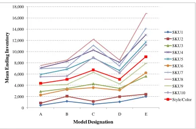
Figure 4.6: Mean Inventory for Representative Category ... 60

Figure 4.7: Pilot test process ... 62

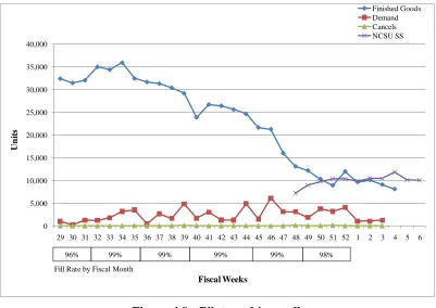
Figure 4.8: Pilot working well ... 63

Figure 4.9: Pilot working well until new inventory policy abandoned ... 63

(22)

Figure 4.11: SKUs at 95% Fill Rate for Pilot Test ... 65

Figure 4.12: As Inventory Levels Reduce Problems are Revealed ... 65

Figure 4.13: Production Problems when Implemented... 66

Figure 4.14: Finished Goods Inventory Discrepancy ... 67

Figure 4.15: Inventory Levels of a Category the Year the New Policy was Implemented ... 68

Figure 5.1: Apparel Cut & Sew Manufacturing Lead-Time with Sources of Variation ... 70

Figure 5.2: Example Distribution of Lead-Time of an Apparel Cut and Sew Manufacturing

Operation... 71

Figure 5.3: Formulation of Example from Eppen and Martin in Microsoft Excel ... 76

Figure 5.4: Setup of Solver Parameters ... 76

Figure 5.5: The Supply Chain Model for Simulation Study ... 81

Figure 5.6: Theoretical Lead-Time Distribution ... 85

Figure 5.7: Actual Lead-Time Distribution ... 86

Figure 5.8: Actual Bimodal Lead-Time Distribution ... 86

Figure 5.9: Simulation Study Algorithm ... 89

Figure 5.10: Demand and Lost Sales for a SKU Demonstrating a Period of High Lost Sales

Due to a Shift in the Average Demand Near Week 30 ... 97

Figure 5.11: Cycle Service Box Plot for Theoretical Experiments ... 108

Figure 5.12: Fill Rate Box Plot for Theoretical Experiments ... 109

Figure 5.13: Inventory Box Plot for Theoretical Experiments ... 111

Figure 5.14: Cycle Service Box Plot for Modified Theoretical Experiments ... 112

(23)

Figure 5.16: Inventory Box Plot for Modified Theoretical Experiments ... 115

Figure 5.17: Cycle Service Box Plot for Actual Demand Experiments ... 117

Figure 5.18: Fill Rate Box Plot for Actual Demand Experiments ... 119

Figure 5.19: Inventory Box Plot for Actual Demand Experiments ... 120

Figure 5.20: Inventory Box Plot for Actual Demand Experiments – Removing Data Points

(24)

1. Introduction

Market forces demand that companies deliver the correct product to the customer at the

correct time, at the correct location, and at the correct price. Successful companies

implement supply chain strategies that respond to these forces. Today’s competitive markets

challenge companies and their supply chains to balance speed, flexibility, quality, and

responsiveness with low cost.

In the case of the textile and apparel industry, Plunkett’s Research (2006) indicates that

there are sixteen major trends affecting the industry. Some of the trends that directly impact

the textile and apparel supply chain include: “1) Globalization: China dominates apparel and

textiles, 2) Supply chain management evolves to serve the global market, 3) Synthetic fiber

manufacturers face global glut, 4) Mass designers and retailers speed up for fast fashion, and

5) Some apparel manufacturers still resist outsourcing” (Plunkett’s Research 2006).

Many challenges and problems in the business world tend to be complex and difficult

to define since most business systems are human systems. Problems within the business

systems typically stem from the complex relationships inherent in the system. It may be easy

to identify that a problem exists, but understanding and defining the scope of the problem

within a business system is often extremely difficult. In the case of the supply chain, one

such business management problem is the supply chain bullwhip effect.

The bullwhip effect describes a phenomenon in which information about consumer

demand becomes increasingly distorted as it moves up the supply chain from retailers to

(25)

perturbations at distinct levels within the supply chain. The distortions in the perception of

demand within the supply chain make it difficult to match supply to actual demand, which

results in higher costs, product shortages/overages, finished goods obsolescence,

unpredictable orders, and excessive capacity.

Although the ultimate consumer demand is relatively stable at the retailer, the

demand becomes increasingly variable as it advances up the supply chain (retailer to

wholesaler, wholesaler to manufacturer, and manufacturer to supplier). In general, the orders

to suppliers have a larger variance than sales to the buyers. This variance is amplified as

orders propagate up the supply chain in part due to distortions in the chain (length of the

chain, shipping times, lead times, etc.) (Maltz 2001). In terms of lead-time, the supply chain

members furthest from the end customer generally experience the highest variation in

demand.

Figure 1.1: Illustrative Example of Demand Perturbations at Distinct Levels within the Supply Chain 0 20 40 60 80 100

1 6 11 16 21 26 31 36 41 46

Dem

and

Time Consumer Demand at Retailer

0 20 40 60 80 100

1 6 11 16 21 26 31 36 41 46

D e m a n d Time

Demand at Wholesaler

0 10 20 30 40 50 60 70 80 90 100

1 5 9 13 17 21 25 29 33 37 41 45 49

D e m a n d Time Demand at Manufacturer

0 10 20 30 40 50 60 70 80 90 100

1 4 7 10 13 16 19 22 25 28 31 34 37 40 43 46 49

Dem

and

Time

(26)

The lead-time of information and material is the primary root cause of the bullwhip

effect since the information regarding a change in end customer demand is delayed in time as

the information propagates through the supply chain (Lee et. al. 1997). As a result, the

demand experienced by the supply chain members furthest from the end customer can be

significantly out of phase in time and magnitude with true end user demand. Therefore,

suppliers are reacting to a demand that may or may not be the same as the current end

customer demand. Confounding this issue is the time required for suppliers to adjust their

manufacturing capacities and inventories in reaction to the information regarding a change in

demand. Suppliers can find themselves riding a wave of increasing capacities and

inventories immediately followed by reductions in capacity and inventory. The time required

to accomplish these changes in capacity and inventory reduces the supplier’s ability to

appropriately react to the true change in demand. Thus, the bullwhip effect increases with

longer lead-times.

The preceding discussion of the bullwhip effect exemplifies the complex and difficult

problems and challenges faced by today’s industry. In this dissertation, methods of

addressing such supply chain management problems are presented. Chapter two further

describes the challenges faced by industry and focuses upon supply chain performance

measures. A measurement framework is presented for supply chains employing continuous

improvement strategies such as Lean. Chapter three puts forward a method of addressing

difficult supply chain problems. The method employs two tools from the Theory of

Inventive Problem Solving (TRIZ) methodology: the system operator and ideality. The

(27)

upon the solution to the inventory problem from chapter three. The development of an

inventory management spreadsheet simulation is described and used to demonstrate the

effectiveness of the new model. Chapter five presents an extension to the inventory model

that incorporates lead-time uncertainty. The performance of the extended model is tested by

enhancing the simulation discussed in chapter four and is shown to provide results

comparable with inventory models from the literature. Finally, chapter six provides a

(28)

2. Supply Chain Performance Measurement

The introduction of this paper described a set of challenges faced by today’s industry.

To meet these challenges and thus to be a competitive power in their industry, some

companies are implementing strategies such as lean manufacturing, just-in-time, and six

sigma (Porter 2001). Porter (2001) states, “today’s competitive realities demand leadership.”

Additionally, he states, “leaders believe in change” and “[leaders] energize their

organizations to continuously innovate.” One way companies can seek competitive

advantage is to implement Lean manufacturing (Lean) or similar continuous improvement

strategies. These strategies empower company’s leadership to foster change, continuous

improvement, and innovation.

While meeting the aforementioned challenges, companies must continue to generate

profit. In order to monitor profitability and financial wellbeing, companies employ a litany

of well-publicized financial measures such as return on investment, earnings per share, net

profit, and cash flow. These financial measures are important in assessing the financial

health of a business, but “tend to be historically oriented, lacking forward-looking

perspective” (Lapide 2000). Meyer (1996) states that “financial measures summarize past

performance well but predict future performance poorly.” The point addressed by Lapide

and by Meyer highlights an important implication for lean manufacturing and similar

continuous improvement strategies. Namely, as companies employ Lean, traditional

financial measures fail to gauge the impact to the supply chain in a timely manner and “can

give misleading signals for continuous improvement and innovation” (Kaplan and Norton

(29)

authors have responded with proposed frameworks and approaches for incorporating

non-financial measures to assess supply chain performance (Gunasekaran et al. 2001; Beamon

1999; Neely et al. 1995; Kaplan et al. 1992).

This chapter presents key performance indicators for supply chains that are critical for

Lean and similar continuous improvement strategies. Section one provides an introductory

discussion of supply chains and Lean. Section two presents a review of the supply chain

performance measurement system literature and presents a proposed Lean supply chain

measurement framework. Section three categorizes the various supply chain metrics from

the literature using the proposed framework. Finally, a summary and recommendations for

future work are presented in section four.

2.1 Background

2.1.1 What is a supply chain?

A supply chain consists of all the activities associated with a customer’s request for a

good or service from the transformation and flow of goods from raw materials through to the

customer (Handfield et al. 1999; Chopra et al. 2001). A typical supply chain includes

customers, retailers, distributors, manufacturers, and suppliers. This concept is illustrated in

Figure 2.1. Additionally, the supply chain includes all functional areas within each of the

organizations such as, manufacturing, order procurement, marketing, planning, finance,

customer service, engineering, sales, and distribution. As indicated in Figure 2.1,

(30)

that a supply chain is “a network of linked organizations that come together to fulfill a

customer’s desire for a particular good or service.”

Figure 2.2 shows a partial supply chain for a hosiery manufacturer. The retailer

provides socks to the customer in exchange for funds. The retailer makes replenishment

orders based on consumer demand with the hosiery manufacturer who in turn replenishes the

socks for funds transferred from the retailer. Likewise, the hosiery manufacturer transfers

goods, information, and funds with its suppliers. Similar transactions occur throughout the

supply chain as a result of consumer demand for the socks. Thus, large amounts of

information, goods, and funds are transferred up and down the supply chain in an effort to

satisfy consumer demand for socks.

CUSTOMERS

RETAILER

DISTRIBUTOR

MANUFACTURER

SUPPLIER SUPPLIER

SUPPLIER

SUPPLIER SUPPLIER

Double arrow indicates the flow of goods and information up and down the supply chain.

Figure 2.1: Conceptual model of a supply chain

(31)

Figure 2.2: Partial Supply Chain for a Hosiery Manufacturer

(Adapted from Martin et al. 2004)

2.1.2 What is Lean?

Lean is a business strategy, based upon the Toyota Production System, which strives to

continuously improve processes by eliminating waste. Taiichi Ohno is generally credited

with developing the Toyota Production System. Ohno (1988) identified seven types of

waste: overproduction, waiting, transportation, processing, inventories, moving, and defects.

Within the context of a supply chain, the elimination of the seven wastes through continuous

improvement of processes leads to becoming a time-based competitor (Cunningham and

Fiume 2003). The primary tenants of Lean can be summarized as customer service, waste

elimination, and speed.

Three core Lean principles for waste elimination are: pull, flow, and takt time

(Cunningham and Fiume 2003). Pull seeks to produce only what the customer is buying

rather than producing to bet (commonly referred to as produce to forecast). Pull initiates

Farmer Cotton Gin _ManufacturerYarn _ManufacturerHosiery Retailer Customer

Synthetic Manufacturer

Chemical Manufacturer

Cardboard Manufacturer

Lumber Company

(32)

production after receiving or fulfilling a customer’s order as opposed to producing to

inventory in anticipation of a customer’s order. Flow seeks to increase the velocity of the

production process by eliminating queues, handling, movement, and other non-value added

activities and processes. Takt time is the rate of finished product completion. The

customer’s buying rate establishes takt time. Production capacity should be adjusted to takt

time, thus limiting overproduction and underproduction.

George (2002) summarizes Lean as follows: “Lean means speed.” He goes on to say

that Lean seeks to deliver products with “high velocity, high quality, low cost, and minimal

invested capital” (George 2002). In summary, Lean is a strategy that seeks to deliver the

correct product to the customer at the correct time, at the correct location, and at the correct

price with minimal waste. Therefore, one could summarize the core principles of Lean as

customer focus, waste elimination, and speed.

2.1.3 Background Summary

Lean can provide significant positive impact when applied to a supply chain. As

previously discussed, supply chains exist to fulfill a customer’s desire for a particular

product. Lean supply chains deliver that product with speed, quality, and low cost. As

supply chains convert to Lean, supply chain managers must have performance measurement

frameworks to measure progress and to ensure successful Lean transformation. The next

(33)

2.2 Framework for Supply Chain Performance Measurement

2.2.1 Review of Previous Work

Over the past few decades, the pressures of the modern business environment have

increased the importance of supply chain management. Supply chain management has

become common practice across all industries (Chan et al. 2003). Authors, such as Lee and

Billington (1992), point out the necessity of adequately measuring the performance of supply

chains as an important component of supply chain management. Neely et al. (1995) defines

performance measurement as the process of quantifying the efficiency and effectiveness of

action. Performance measurement provides the feedback mechanism for measuring progress

and ensuring achievement of strategic supply chain goals.

Previous work in the supply chain performance measurement system literature can be

generally categorized into the following primary areas: 1) categorization of supply chain

metrics and performance measures, 2) development of balanced scorecard frameworks, and

3) development of new frameworks and measures focused on general application and

evaluation of supply chain models. Neely et al. (1995) state that measurement frameworks

have been developed and others have provided criteria for the measurement system design.

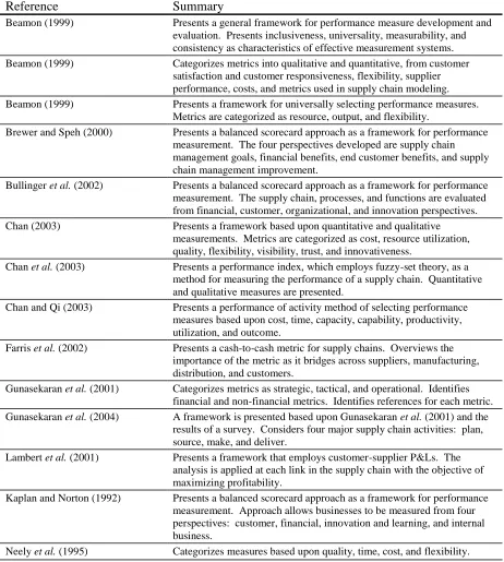
Table 2.1 summarizes the primary contributions to performance measurement systems by

various authors.

Beamon (1998) broadly classifies performance measures as quantitative and qualitative.

Neely et al. (1995) narrow the categories to quality, time, flexibility, and cost. Whether

(34)

an effective and logical mechanism for analyzing and communicating the large number of

metrics and performance measures available for supply chains.

The balanced scorecard frameworks are based upon tracking critical measures that

focus on the company’s strategy. Kaplan and Norton (1992) compare the balanced scorecard

to the “dials in an airplane cockpit that give managers complex information at a glance.”

Brewer and Speh (2000) assert, “Only those who understand the interrelationship between

[supply chain management and the balanced scorecard] will have a greater likelihood of

leveraging their supply chains into a source of competitive advantage.” Kaplan and Norton

(1992), Brewer and Speh (2000), and Bullinger et al. (2002) provide more detailed

discussion on balanced scorecard performance measurement frameworks.

Previous work includes the development of new frameworks and measures focused on

general application and evaluation of supply chain models. Beamon (1999) presents a

framework for universally selecting performance measures in which she identifies three types

of measures: resources, output, and flexibility. Gunasekaran et al. (2001) develops a

framework for measuring strategic, tactical, and operational levels of performance in a

supply chain. Most of the proposed frameworks focus on the selection of performance

measures or develop generalized performance measures and indexes. The shortcomings of

these frameworks establish a need for a new framework for lean supply chains as will be

(35)

Table 2.1: Summary of the primary contributions to performance measurement systems

Reference Summary

Beamon (1999) Presents a general framework for performance measure development and evaluation. Presents inclusiveness, universality, measurability, and consistency as characteristics of effective measurement systems. Beamon (1999) Categorizes metrics into qualitative and quantitative, from customer

satisfaction and customer responsiveness, flexibility, supplier performance, costs, and metrics used in supply chain modeling. Beamon (1999) Presents a framework for universally selecting performance measures.

Metrics are categorized as resource, output, and flexibility.

Brewer and Speh (2000) Presents a balanced scorecard approach as a framework for performance measurement. The four perspectives developed are supply chain management goals, financial benefits, end customer benefits, and supply chain management improvement.

Bullinger et al. (2002) Presents a balanced scorecard approach as a framework for performance measurement. The supply chain, processes, and functions are evaluated from financial, customer, organizational, and innovation perspectives.

Chan (2003) Presents a framework based upon quantitative and qualitative measurements. Metrics are categorized as cost, resource utilization, quality, flexibility, visibility, trust, and innovativeness.

Chan et al. (2003) Presents a performance index, which employs fuzzy-set theory, as a method for measuring the performance of a supply chain. Quantitative and qualitative measures are presented.

Chan and Qi (2003) Presents a performance of activity method of selecting performance measures based upon cost, time, capacity, capability, productivity, utilization, and outcome.

Farris et al. (2002) Presents a cash-to-cash metric for supply chains. Overviews the importance of the metric as it bridges across suppliers, manufacturing, distribution, and customers.

Gunasekaran et al. (2001) Categorizes metrics as strategic, tactical, and operational. Identifies financial and non-financial metrics. Identifies references for each metric.

Gunasekaran et al. (2004) A framework is presented based upon Gunasekaran et al. (2001) and the results of a survey. Considers four major supply chain activities: plan, source, make, and deliver.

Lambert et al. (2001) Presents a framework that employs customer-supplier P&Ls. The analysis is applied at each link in the supply chain with the objective of maximizing profitability.

Kaplan and Norton (1992) Presents a balanced scorecard approach as a framework for performance measurement. Approach allows businesses to be measured from four perspectives: customer, financial, innovation and learning, and internal business.

(36)

Table 2.1 continued

Stewart (1995) Presents a framework based upon plan, source, make, and deliver. Identifies keys to unlocking supply chain excellence as delivery performance, flexibility and responsiveness, logistics cost, and asset management.

van Hoek (1998) Presents three fundamental steps for development of new measurement systems: provide a context for measurement, create benchmarks based upon new measures, and development of tools that support the measures.

2.2.2 The Need for a Performance Measurement Framework for Lean Supply Chains

Brewer and Speh (2000) state that if companies “continue to evaluate employees using

performance measurement systems that are either adversely affected by or completely

unaffected by supply chain improvements, then they will fail in their supply chain

endeavors.” Lean is a continuous improvement strategy that significantly impacts the supply

chain. Furthermore, Lean improvement activities can adversely affect traditional financial

measures. For example, reducing inventory releases deferred cost from the balance sheet to

the profit and loss statement; thus generating a short-term decrease in profit. In this example,

the act of improving inventory levels generated an adverse effect in the profit and loss

statement. Thus, a performance measurement framework for Lean supply chains is needed to

ensure success in supply chain improvement activities.

Chan (2003) points out several problems with existing performance measurement

frameworks in the supply chain context. He asserts that most measurements are not

connected with strategy and are financially biased. Additionally, the measurements lack a

(37)

addition to these problems, existing performance measurement frameworks have the

following shortcomings:

1. Propose measures that are difficult to quantify;

2. Advocate index measures that have little or no context for interpretation;

3. Propose too many measures.

A performance measurement framework for Lean supply chains is needed that 1)

connects the performance measurements with the tenets of a Lean strategy, 2) balances

financial and non-financial measures, and 3) utilizes a small number of quantifiable and

meaningful measures. The next section of this chapter proposes a framework for Lean

supply chains utilizing these criteria.

2.2.3 Proposed Framework for Lean

The main challenge when developing a performance measurement framework is

determining the proper measures to include. Thor (1994) suggests that there should be a

balanced collection of four to six performance measures, typically including productivity,

quality, and customer satisfaction. Meyer (1996) proposed the following set of criteria for

configuring measures:

1. There should be three to six measures for tracking towards the strategic goals

(enough to make gaming difficult but not too many to confuse).

2. There should be a mix of financial and non-financial measures.

3. There should be constraints between measures. The constraints should ensure that a

gain in any one of the measures genuinely reflects performance improvement.

(38)

achieved at the expense of another. Nor should the measures be so relaxed that

gains in one automatically mean gains in the others.

Cunningham and Fiume (2003) list the following attributes of a good performance

measurement framework:

1. Support the company’s strategy.

2. Be relatively few in number.

3. Be mostly non-financial.

4. Be structured to motivate the right behavior.

5. Be simple and easy to understand.

6. Not combine measures of different things into a single index.

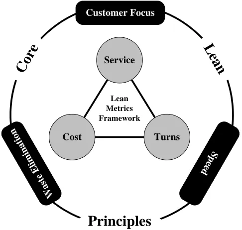
The proposed framework for Lean supply chains consists of the following three

performance measures: customer service, inventory turns, and total cost. The premise for

selecting these three measures is based upon the aforementioned criteria given by Meyer

(1996) and Cunningham and Fiume (2003).

The measures proposed for the Lean framework directly tie to the core principles of a

Lean supply chain strategy. The tenets of Lean were previously summarized as customer

focus, waste elimination, and speed. Figure 2.3 illustrates the relationship between these

principles and the proposed performance measures that constitute a framework for Lean

supply chains. Customer focus is tied primarily to the customer service measure. Customer

service measures the ability of the supply chain to meet the customer’s needs in a timely

manner. Waste elimination is primarily associated with total cost. As waste is eliminated

(39)

Lean Metrics Framework

Service

Cost Turns

Customer Focus

S p ee d

W as te E li m in at io n

C

or

e

L

_ea

n

Principles

Figure 2.3: A performance measurement framework for Lean supply chains

(Original work)

primarily tied to inventory turns. Increasing the velocity of the supply chain will result in

higher inventory turns.

In addition to being clearly tied to a Lean strategy, the selected measures motivate Lean

behavior. Norton and Kaplan (1992) stated, “You get what you measure.” The profundity of

this five-word sentence cannot be overemphasized. Quite simply, employee behavior is

motivated by the measures upon which their performance is assessed. Therefore, by

measuring and by making employees accountable for the results of customer service,

inventory turns, and total cost, the Lean performance measurement framework motivates the

desired employee behavior that contributes to the Lean principles of customer focus, waste

(40)

The performance measurement framework for Lean supply chains includes three

measures that mutually constrain one another. The framework includes enough measures to

make gaming difficult, but not too many that result in confusion. For the purpose of this

chapter, gaming refers to the intentional manipulation of the supply chain to achieve a

desired result in a particular measure. For example, intentionally producing items for which

there is no demand, in order to improve a fixed cost per unit measure, would be considered

gaming. The constraints between customer service, inventory turns, and total cost make

gaming difficult. In the case of customer service, an increase cannot be obtained only by

carrying additional inventory because the additional inventory would negatively impact

inventory turns and total cost. Likewise, total cost cannot be improved by producing items

for which there is no demand because inventory turns will worsen. Also, a reduction in

inventory for the purpose of improving inventory turns may negatively impact customer

service. Therefore, the measures of customer service, inventory turns, and total cost

sufficiently constrain one another. However, the constraints between the measures provide

enough slack to permit improvement in one without necessarily negatively impacting

another.

The performance measurement framework, shown in Figure 2.3, establishes a small set

of mutually constraining measures that are clearly linked to a Lean supply chain strategy.

Customer service, inventory turns, and total cost are the key performance indicators for a

Lean supply chain. Simply put, an organization must do a lot of things correct, inclusive of

(41)

Customer service, inventory turns, and total cost are the key performance indicators for

top-level supply chain management to track and to assess Lean improvement activities.

However, other metrics should be tracked at lower levels of the organization. These metrics

should be aligned with the measures that constitute the performance measurement framework

for Lean supply chains. The next section of this chapter categorizes various measures from

the supply chain measurement literature using the performance measurement framework for

Lean supply chains.

2.3 Lean Supply Chain Performance Indicators

2.3.1 Customer Service

Customer service gauges an organization’s ability to supply the needs of the customer.

Customer service is the primary driver of customer satisfaction, which is the most

controllable by an organization (Stewart 1995). To be deemed effective, a supply chain

strategy must satisfy the customer. Lee and Billington (1992) and van Hoek et al. (2001)

emphasize the importance of including customer satisfaction centric metrics for assessing

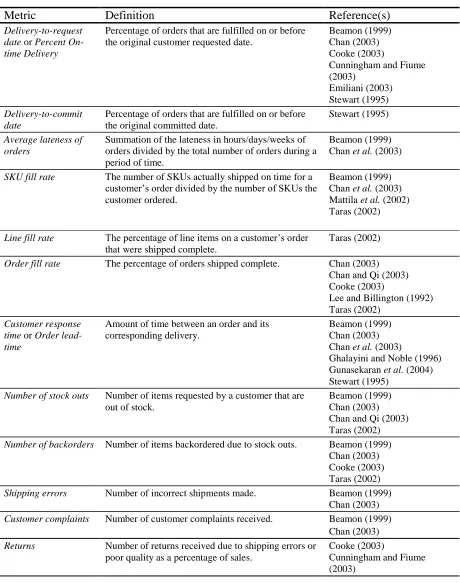
supply chain performance. Table 2.2 provides some of the supply chain metrics from the

(42)

Table 2.2: Some of the supply chain metrics that contribute to customer service

Metric Definition Reference(s)

Delivery-to-request date or Percent On-time Delivery

Percentage of orders that are fulfilled on or before the original customer requested date.

Beamon (1999) Chan (2003) Cooke (2003)

Cunningham and Fiume (2003)

Emiliani (2003) Stewart (1995)

Delivery-to-commit date

Percentage of orders that are fulfilled on or before the original committed date.

Stewart (1995)

Average lateness of orders

Summation of the lateness in hours/days/weeks of orders divided by the total number of orders during a period of time.

Beamon (1999) Chan et al. (2003)

SKU fill rate The number of SKUs actually shipped on time for a customer’s order divided by the number of SKUs the customer ordered.

Beamon (1999) Chan et al. (2003) Mattila et al. (2002) Taras (2002)

Line fill rate The percentage of line items on a customer’s order that were shipped complete.

Taras (2002)

Order fill rate The percentage of orders shipped complete. Chan (2003) Chan and Qi (2003) Cooke (2003)

Lee and Billington (1992) Taras (2002)

Customer response time or Order lead-time

Amount of time between an order and its corresponding delivery.

Beamon (1999) Chan (2003) Chan et al. (2003)

Ghalayini and Noble (1996) Gunasekaran et al. (2004) Stewart (1995)

Number of stock outs Number of items requested by a customer that are out of stock.

Beamon (1999) Chan (2003) Chan and Qi (2003) Taras (2002)

Number of backorders Number of items backordered due to stock outs. Beamon (1999) Chan (2003) Cooke (2003) Taras (2002)

Shipping errors Number of incorrect shipments made. Beamon (1999) Chan (2003) Customer complaints Number of customer complaints received. Beamon (1999)

Chan (2003)

Returns Number of returns received due to shipping errors or poor quality as a percentage of sales.

Cooke (2003)

(43)

Table 2.2 continued

Order entry accuracy Percentage of orders entered without error. Taras (2002) Customer query time The time it takes to respond to a customer query

with the required information.

Gunasekaran et al. (2001) Gunasekaran et al. (2004) Perfect order The percentage of orders filled flawlessly. Cooke (2003)

Lapide (2000) Taras (2002)

2.3.2 Inventory Turns

Inventory turns is generally defined as the annualized cost of goods sold (COGS)

divided by the average inventory level for the period. The measure indicates the number of

times inventory turns over for a given sales volume. Low inventory turns indicate an

inefficient supply chain. Contrarily, high inventory turns “means the business has achieved

high velocity and eliminated significant waste throughout the organization” (Cunningham

and Fiume 2003). Many factors within the supply chain can affect inventory turns including

inventory levels, manufacturing lead-times, supplier lead-times, capacity utilization,

inventory policy, manufacturing strategy and philosophy (push versus pull), and financial

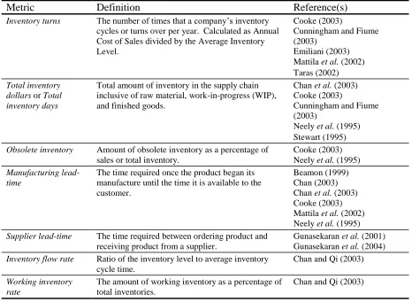
measures (for example, fixed cost per hour). Table 2.3 summarizes some of the supply chain

(44)

Table 2.3: Some of the supply chain metrics that affect inventory turns

Inventory turns The number of times that a company’s inventory cycles or turns over per year. Calculated as Annual Cost of Sales divided by the Average Inventory Level.

Cooke (2003)

Emiliani (2003) Mattila et al. (2002) Taras (2002) Total inventory

dollars or Total inventory days

Total amount of inventory in the supply chain inclusive of raw material, work-in-progress (WIP), and finished goods.

Chan et al. (2003) Cooke (2003)

Neely et al. (1995) Stewart (1995) Obsolete inventory Amount of obsolete inventory as a percentage of

sales or total inventory.

Cooke (2003) Neely et al. (1995) Manufacturing

lead-time

The time required once the product began its manufacture until the time it is available to the customer.

Beamon (1999) Chan (2003) Chan et al. (2003) Cooke (2003) Mattila et al. (2002) Neely et al. (1995) Supplier lead-time The time required between ordering product and

receiving product from a supplier.

Gunasekaran et al. (2001) Gunasekaran et al. (2004) Inventory flow rate Ratio of the inventory level to average inventory

cycle time.

Chan and Qi (2003)

Working inventory rate

The amount of working inventory as a percentage of total inventories.

Chan and Qi (2003)

2.3.3 Total Cost

Total cost is the measure of fixed costs and variable costs associated with the resources

required to plan, make, and deliver a product. Total cost can be used to measure the

efficiency of a supply chain due to the inclusiveness of all functional areas within a supply

chain. The measure helps to assess the impact of actions to influence in one area in terms of

the impact on costs associated with other areas (Cavinato 1992). For example, a decision to

reduce inventory could have a major impact on costs associated with capacity utilization.

(45)

2.3.4 Summary of Lean supply chain performance indicators

The primary performance indicators for a Lean supply chain are customer service,

inventory turns, and total cost. Each of these measures ties directly to the core lean

principles of customer focus, speed, and waste elimination respectively. The key

performance indicators should be tracked at the senior levels of the supply chain

management organization. This section of the paper summarizes some of the measures that

contribute to each of the key performance indicators that should be tracked at lower levels of

the supply chain management organization. Hofman et al. (2005) presents a metrics

architecture that defines metrics that matter for the different areas of an organization. The

architecture is based upon a performance pyramid. As a means of summary, Figure 2.4

illustrates a possible metric architecture combing the proposed framework for performance

measurement for Lean supply chains and the architecture advocated by Hofman et al. (2005).

The alignment of the sub-metrics to the key performance indicators and thus the Lean supply

(46)

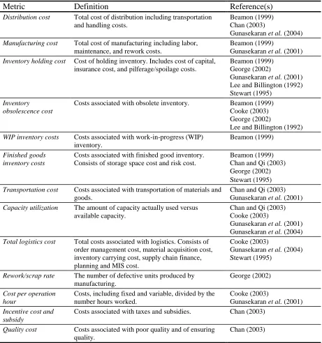
Table 2.4: Some of the supply chain metrics that contribute to total cost

Distribution cost Total cost of distribution including transportation and handling costs.

Beamon (1999) Chan (2003)

Gunasekaran et al. (2004)

Manufacturing cost Total cost of manufacturing including labor, maintenance, and rework costs.

Beamon (1999)

Gunasekaran et al. (2001) Inventory holding cost Cost of holding inventory. Includes cost of capital,

insurance cost, and pilferage/spoilage costs.

Beamon (1999) George (2002)

Gunasekaran et al. (2001) Lee and Billington (1992) Stewart (1995)

Inventory obsolescence cost

Costs associated with obsolete inventory. Beamon (1999) Cooke (2003) George (2002)

Lee and Billington (1992) WIP inventory costs Costs associated with work-in-progress (WIP)

inventory.

Beamon (1999)

Finished goods inventory costs

Costs associated with finished good inventory. Consists of storage space cost and risk cost.

Beamon (1999) Chan and Qi (2003) George (2002) Stewart (1995) Transportation cost Costs associated with transportation of materials and

goods.

Chan and Qi (2003) Gunasekaran et al. (2001)

Capacity utilization The amount of capacity actually used versus available capacity.

Chan and Qi (2003) Cooke (2003)

Gunasekaran et al. (2001) Gunasekaran et al. (2004) Total logistics cost Total costs associated with logistics. Consists of

order management cost, material acquisition cost, inventory carrying cost, supply chain finance, planning and MIS cost.

Cooke (2003)

Gunasekaran et al. (2004) Stewart (1995)

Rework/scrap rate The number of defective units produced by manufacturing.

George (2002)

Cost per operation hour

Costs, including fixed and variable, divided by the number hours worked.

Cooke (2003)

Gunasekaran et al. (2001) Incentive cost and

subsidy

Costs associated with taxes and subsidies. Chan (2003)

Quality cost Costs associated with poor quality and of ensuring quality.

(47)

Service Fill Rate On-time Delivery Number of Backorders Number of Stockouts Order Lead Time Customer Complaints Customer Query Time Shipping Errors Perfect Order Key Performance Indicator Sub-Metrics Customer Focus Turns Inventory Turns Total Inventory Supplier Lead-time Manufacturing Lead-time Inventory Days Inventory Flow Rate Working

Inventory Rate COGS

Obsolete Inventory Key Performance Indicator Sub-Metrics Speed Cost Cost of Distribution Cost of Inventory Cost of Obsolescence Manufacturing Cost WIP Cost Cost of Transportation Capacity Utilization Scrap Rate Cost Per Hour Key Performance Indicator Sub-Metrics Waste Elimination

Figure 2.4: Examples of performance metric pyramids for Lean supply chains

(Adapted from: Hofman et al. 2005)

2.4 Summary

Performance measures are critical for the successful implementation and assessment of

a supply chain strategy. As organizations implement Lean and other continuous

improvement strategies to meet the needs of today’s marketplace, traditional financial

measures and performance measurement frameworks fail to properly gauge the benefits. In

order to reflect the benefits of such strategies, a performance measurement framework for

Lean supply chains is needed.

Previous work in the area of performance measurement frameworks has the following

problems with respect to Lean:

(48)

lack a balanced approach to integrating financial and non-financial measures

(Chan 2003);

propose measures that are difficult to quantify;

advocate index measures that have little or no context for interpretation;

propose too many measures.

This chapter discusses the importance of a performance measurement framework for

Lean supply chains that ties to the core lean principles of customer service, waste

elimination, and speed. The framework presented in this chapter 1) connects the

performance measurements with the tenets of a Lean strategy, 2) balances financial and

non-financial measures, and 3) utilizes a small number of quantifiable and meaningful measures.

Art Byrne, former CEO of Wiremold during their lean transformation, said “if he were

forced to use just two metrics for the entire company, he would choose customer service and

inventory turns” (Cunningham and Fiume 2003). The framework presented in this chapter

adds total cost to Art Byrne’s list. Customer service, inventory turns, and total cost are the

key performance indicators for top-level supply chain management to track and assess Lean

improvement activities. However, other metrics should be tracked at lower levels of the

organization. Therefore, this chapter presents a categorization of additional metrics from the

literature that contributes to the three key performance indicators included in the framework

(49)

3. Solving a Real World Inventory Management Problem Using a Technique for Integrating Ideality with the System Operator

Martin, Benjamin R., J. Joines, and T. G. Clapp. “Solving a Real World Inventory

(50)

3.0 Introduction

Difficult and enigmatic problems can be found in the functional areas of supply chain

management. Examples of such problem areas include: demand forecasting, raw material

inventory planning, customer management, inventory allocation, order management,

manufacturing planning, capacity planning, marketing, pick management, distribution,

transportation, plant and shop floor scheduling, and finished goods inventory planning. Each

of these areas yields difficult problems to solve – owing in part to the complex

interrelationships between the functional areas. The existence of a supply chain management

problem may be easily identified, but the scope, complexity, and ultimate solution are often

difficult to define. Finished goods inventory planning is a prime example. Within the

functional area of finished goods inventory planning, the amount of inventory to be carried

must be determined such that inventory is minimized while fulfilling customer orders at an

acceptable rate or customer service level. Other supply chain areas such as forecasting,

capacity planning, transportation, distribution, manufacturing, and marketing significantly

influence the amount of finished goods inventory to maintain. The complex

interrelationships between finished goods inventory planning and other supply chain function

areas present challenges for understanding, defining, and ultimately solving problems.

The Theory of Inventive Problem Solving (TRIZ) provides numerous tools for

solving problems such as the finished goods inventory planning just described. In particular,

the system operator and ideality are two TRIZ tools that provide systematic and methodical

approaches to understanding and defining a problem that leads to solution generation. The

(51)

be integrated to produce a methodical and systematic solution generation technique (Martin

et al. 2004). The technique defines a tool that identifies resources at each of the interfaces

delineated by the system operator matrix. This chapter discusses the application of the

technique for integrating the system operator with ideality to a finished goods inventory

planning problem for a large textile company.

3.1 The System Operator, Ideality, and the Integration Technique

3.1.1 The System Operator

The system operator is a key TRIZ tool that provides a systematic approach for

problem definition and solution generation. The system operator is useful throughout the

problem solving process. The tool may be used for problem definition, idea generation,

solution identification, and solution implementation. The TRIZ literature suggests that the

system operator is used under a variety of different conditions: 1) to define the problem, 2) to

look for the solution to a problem, and 3) to determine the trend of a system development

(Frenklach 1998).

The system operator directs thinking in terms of time and space by dividing the

problem into three levels and three time zones (Mann 2001). The three levels comprise the

system, super-system, and subsystem. The three times zones suggested by the system

operator are the past, present and future. The division results in a three-by-three matrix as

shown in Figure 3.1. Each box represents a particular space and time. The matrix directs

systematic thoughts at each level, thus overcoming “the psychological inertia of present and

(52)

The system, the super-system, and the subsystem levels of the system operator direct

thinking outside of the system itself and into the system’s environment and sub-processes. It

is important to not only consider the problem at hand, but also to give consideration to the

environment and sub-processes in which the problem resides as solutions may reside in either

or both of these spaces. The three time zones of the system operator facilitate thinking in

terms of time. The times zones are the past, present, and future. Even though the system

operator breaks time into discrete categories, it is important to continue to think continuously

with respect time. The system operator’s categories provide the systematic framework for

thinking in terms of time. Thus, the combination of space and time in the system operator

helps to think more completely about the problem to be solved thus maximizing solution

generation possibilities.

Figure 3.1: The system operator matrix

Past Super System

Present Super System

Future Super System

Past System

Present System

Future System

Past Sub-System

Present Sub-System