An Interactive Framework for The Parameter Design Problem

(1)

Abstract

AKHAVAN TABATABAEI, RAHA. AN INTERACTIVE FRAMEWORK FOR THE

PARAMETER DESIGN PROBLEM. (Under direction of Dr. Yahya Fathi.)

We propose an interactive framework for solving the Parameter Design Problem. In

this context we consider a response functionY =h(x₁,...,x_n), where x₁,...,x_n are random

variables with known probability distribution functions, and h is a continuous and

differentiable function. Given the distribution functions of x1 through xn and the function

h, we use a family of Johnson distributions to approximate the probability density

function of Y by using its first four moments as input. This density function can be

displayed graphically and compared with the given specification limit of Y. Using this

approach we develop a computer program that would allow the user to modify the set

points of x₁,...,x_n manually, and immediately observe the impact of this adjustment on

the probability density function of Y. The user can then interactively search for and

determine a satisfactory set of values for these set points. We also present two case

studies and solve them by this method. The framework that we propose also provides a

platform for employing other techniques such as nonlinear programming or statistical

design of experiment in order to assist the user in determining a satisfactory solution for

(2)

An Interactive Framework for The

Parameter Design Problem

By

Raha Akhavan Tabatabaei

A thesis submitted to the Graduate Faculty of North Carolina State University

in partial fulfillment of the requirements for the Degree of Master of Science

Industrial Engineering

Raleigh

2005

APPROVED BY:

(3)

Biography

(4)

µ₁,...., are controllable parameters (i.e., their values can be determined by the design engineer). In the design phase values of µ₁,....,µ_nare determined such that the nominal value of Y is equal to its target value,τ . During the production phase, existence of noise can cause values of x₁....x_n to deviate from their set pointsµ₁,....,µ_n, hence causing Y to deviate form its target value,τ .

Parameter Design Problem focuses on determining µ₁,....,µ_nsuch that not only nominal value of Y is kept on target, but also the variation or noise in Y is minimized.

1.2 Literature Review

(10)

This methodology is based on using an orthogonal array in experimental design to maximize signal to noise ratio. Fathi [6] states the advantages of this method in being modest in computational requirements and suitable for the situations where the analytical form of the response function between the design variables and the output characteristic Y

is not available. The major disadvantage is also stated as terminating at a suboptimal solution.

Box and Fung [2] proposed a constrained nonlinear programming (NLP) model to maximize the signal to noise ratio, and showed that when applicable, this model could result in better solutions. Fathi [7] proposed a constrained nonlinear programming model that minimizes the variance of Y. In this method variance of Y is approximated by

successive quadratic approximations of the response function. This is only applicable to cases where the response function is known or can be well approximated.

Another approach proposed by Fathi [6] approximates the variance of Y by using a linear approximation. He uses Taylor series expansion to approximate h up to its linear term. From there, mean and variance of h are calculated about the point (µ₁....µ_n). Then he uses this approximation as the objective function of a NLP model. He constrains the problem by forcing nominal value of Y to be on target, and µ₁....µ_n satisfy any other technical requirement (constraint). This methodology is referred to as Parameter Design Model with Linear Approximation of Variance or PDM-LAV.

1.3 The Proposed Model

In this thesis we propose a different approach for solving the Parameter Design Problem. This is an interactive approach in which the design engineer can manually adjust the values of the controllable parameters µ₁....µ_n and see the effect of this adjustment on the probability density function of Y,instantaneously.

In this model, we take advantage of a method of approximating the probability density function of a variate by an empirical distribution. In particular we approximate

probability distribution of Y by a family of Johnson distributions.

(11)

the variate either by using the Taylor series expansion of the function h(x₁,....,x_n)about the set pointsµ₁,....,µ_n , or (as appropriate) by using a Monte-Carlo simulation model. Once the first four moments of Y are evaluated, we identify the Johnson family that it belongs to, and then calculate the distribution parameters of that family. Once the appropriate Johnson family and its parameters are estimated, we form the probability density function (pdf) for Y and plot its graph. Now a design engineer can visually

observe the shape of pdf of Y at the given set points for µ₁,....,µ_n and compare it with the target value of Y and its specification limits. He or she can then try different settings for

n µ

µ₁,...., as appropriate. For each setting that is tried, the pdf of Y is graphed and hence the design engineer can see the effect of this new setting on the pdf of Y. This process continues until a desirable set of values for µ₁,....,µ_n is determined.

1.4 Organization of the Thesis

The empirical distributions and methods of approximation are discussed in Chapter 2. The methods for approximating the first four moments of Y are discussed in Chapter 3. Chapter 4 explains the details of our methodology and the software that is developed for this purpose. In Chapter 5 we present two case studies involving the Parameter Design Model, using this methodology.

The software that we develop can also serve as the basis for a framework in which we may include different approaches in the Parameter Design Problem., i.e. the statistical design of experiments or the nonlinear programming model. In Chapter 6, the features that can be added to the existing model and also other methodologies that can be included in the framework to enhance its capacity and facilitate the search for an optimal

(12)

Chapter 2

Approximation by Empirical Distributions

In this Chapter we discuss methodologies of fitting an empirical distribution to a variate and in particular we focus on the Johnson distributions.

2.1 Background

In the context of the PDP, for a general form of the response functionY =h(x₁,...,x_n), it is usually difficult to determine the exact form of the pdf for Y, even if the exact form of the pdf forx₁,...,x_n is known. In this case we use an approximation of the pdf of Y in our analysis.

One method for approximating the pdf of Y is fitting a well-known distribution such as normal, Gamma, or lognormal. The most common of these methods is the use of normal distribution, since it follows from the central limit theorem that normal distribution provides a reasonable representation of many physical phenomena. Gamma and lognormal distributions are also used for variables which are bounded at one end, and Beta distribution is used for those that are bounded at both ends.

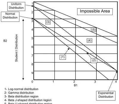
Although these models cover a wide variety of shapes, they do not provide the

desirable degree of generality required. In Figure 2-1, the regions in the(β₁,β₂)plane that are covered by the well-known distributions of lognormal, normal, Beta, Gamma and

student t are shown. In this figure,

2 2 / 3 2 3 1 ) ( _     = σ µ

β represents the square of the

standardized measure of skewness and ₂4 ₂ 2

) (σ

µ

β = represents the standardized measure

of peakedness. In these expressions µ₃ and µ₄ are the third and fourth moments of Y

about its mean, and _σ2_{is its variance.}

(13)

1

2

3

4

B2 5

6

7

8

9

0 1 2 3 4

1- Log-normal distribution 2- Gamma distribution 3- Beta distribution region

4- Beta J-shaped distribution region 5- Beta U-shaped distribution region

Stu

dent t Dis

tr

ibution

B1

Impossible Area

Uniform

Distribution

Normal Distribution

Exponential Distribution (1)

(3)

(2) (4)

(5)

Figure 2-1: (β₁,β₂)plane for well-known distributions.

While this figure can be used for examining the closeness of a given distribution to a well-known distribution (i.e., uniform, normal, etc.), little can be done about the large area that is not occupied by any of these well-known distributions. This justifies the use of empirical distributions.

A more general technique for approximating the pdf of a random variable would be to use either Johnson or Pearson distributions. In this section we discuss Johnson

(14)

2.2 Johnson Distribution

Johnson [11] suggested transforming a standard normal variate as the basis for

empirical distributions. One advantage of this transformation is that we can use a table of areas under a standard normal distribution for estimating the percentiles of the fitted distribution.

The general form of this transformation is [8] : ), , ; ( ε λ ητ γ x

z= + η >0,−∞<γ <∞,λ >0,−∞<ε <∞, (2-1) where x is the variable to be fitted by a Johnson distribution.

In this general form, τ is an arbitrary function, γ,η,ε,λ are the four parameters of Johnson distribution and z is a standard normal variate.

Johnson has proposed the following three families for the functionτ :

(a) ₁( ; , ) ln( ),

λ ε λ

ε

τ x = x− x≥ε, (2-2)

(b) ₂( ; , ) ln( ),

x x x − + − = ε λ ε λ ε

τ ε ≤ x≤ε +λ (2-3)

(c) ( ; , ) sinh 1ln( ),

3 _λ

ε λ

ε

τ _x = − x− ₋_∞_< _x_<_∞ _(2-4)

Hahn and Shapiro [8] find the probability density functions for the three families of Johnson distributions using methods of variable transformation, given that z is a normal variate.

1-Family that corresponds to τ₁ also known as Johnson S_L family:

}, )] ln( [ 2 1 exp{ 2 ) ( ) ( 2 1 _λ ε η γ π ε η ₋ ₊ − − = x x x

f (2-5)

ε ≥

x ,η >0,−∞<γ <∞,λ >0,−∞<ε <∞. Setting γ* ₌γ ₋ηlnλ_gives,

}, )] ln( [ 2 1 exp{ 2 ) ( )

( 2 * 2

1 η γ_η ε

π ε η ₋ ₊ ₋ − = x x x

f (2-6)

ε ≥

(15)

This is in fact a generalized form of the lognormal distribution as described in page 99 in [8]. In most of the literature as well as in the model that we develop in this thesis, equation (2-6) is used as the pdf of S_L family.

2- Family that corresponds to τ₂ also known as Johnson S_B family:

}, )] ln( [ 2 1 exp{ ) )( ( 2 ) ( 2

2 _ε _λλ _ε γ η _λ ε _ε

π η + − − + − + − − = x x x x x

f (2-7)

. , 0 , , 0

, > −∞< <∞ > −∞< <∞ +

≤

≤ λ ε η γ λ ε

ε x

3-Family that corresponds to τ₃ also known as Johnson S family: _U

], }) ] 1 ) [( ) ln{( ( 2 1 exp[ ) ( 1 2 )

( 2 1/2 2

2 2 3 + − + − + − + − = λ ε λ ε η γ λ ε π

η x x

x x

f (2-8)

. , 0 , , 0

, > −∞< <∞ > −∞< <∞ ∞

< < ∞

− x η γ λ ε

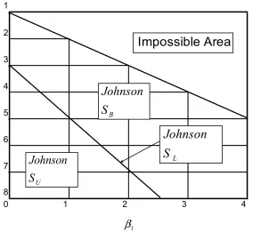
Hahn and Shapiro [8] also show the(β₁,β₂) plane for these Johnson families.

1 2 3 4 5 6 7 8

0 1 2 3 4

Impossible Area

B

S

Johnson

U

S

Johnson

S

L

Johnson

1 β

(16)

Note that the Johnson S_Land S_Bfamilies both have two shape parameters γ andη, one location parameterε, and one scale parameterλ.

From the defined range of the random variate x in each family, we can see that S_U,S_L

and S_B distributions are defined for unbounded variates, variates bounded at one end, and variates bounded from both above and below, respectively. However these

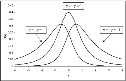
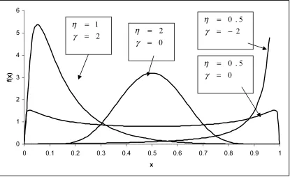
limitations need not be strictly followed when the distributions are used for approximation. This is similar to approximating a bounded variate with normal distribution which is unbounded by nature. Figures 2-3, 2-4, and 2-5show some examples of curves from the S_U,S_L_andS_B families, respectively. It can be observed that these families of distributions give a wide range of shapes; hence they can be used in a variety of situations.

0 0.05 0.1 0.15 0.2 0.25 0.3 0.35 0.4 0.45

-4 -3 -2 -1 0 1 2 3 4

x

f(x

)

Figure 2-3: Johnson S_Udistributions with ε =0,λ=1and various values of the parameters ηandγ .

1 ,

1 =

= γ η

0 ,

1 =

= γ η

1 ,

1 =−

(17)

0 0.1 0.2 0.3 0.4 0.5 0.6 0.7

0 2 4 6 8 10

x

f(

x)

Figure 2-4: Johnson S_Ldistributions with ε =0and various values of the parameters ηandγ*.

0 1 2 3 4 5 6

0 0.1 0.2 0.3 0.4 0.5 0.6 0.7 0.8 0.9 1

x

f(

x)

Figure 2-5: Johnson S_Bdistributions with ε =0,λ=1and various values of the parameters ηandγ . 0 2 = = γ η 0 5 . 0 = = γ η 2 5 . 0 − = = γ η 2 1 = = γ η 0 , 1 * ₌ = γ η 3 . 0 ,

1 * ₌₋ = γ η

1 ,

(18)

2.3 Approximation by Johnson Distribution

In order to approximate a variate, Y, using Johnson distributions, we must first determine its corresponding family of Johnson distribution and then determine the parameters of that family. To this end we need to determine the values ofβ₁ andβ₂, and identify the point (β₁,β₂)in Figure 2-2. If the (β₁,β₂)point falls close to the log-normal line, then S_Lis chosen. If it falls above or below this line, then S_Bor S_U should be chosen, respectively. The range of the regions in Figure 2-2 can be extended by use of these parametric equations

( 1)( 2)2,

1 = ω− ω+

β (2-9)

4 2 3 3 2 3

2 =ω + ω + ω −

β . (2-10) Additional points can be obtained by choosing values for ωand solving for the

corresponding values of β₁ andβ₂, as we discuss later.

To determine parameters of the fitted Johnson distribution (i.e.γ,η,λ,ε), two different approaches are used in the literature. One method is based on using a relatively large random sample. This method is discussed in [8] in details. The second approach, which is used in this thesis, is based on using the first four moments of the random variate Y. This method is proposed by Hill, Hill and Holder in [9], where they provide the details of this algorithm and a corresponding computer program. This program takes the mean, the standard deviation, the skewness and the peakedness of a variate as its input. With this input, the algorithm finds the family of Johnson distribution that fits the variate and then calculates the parameters of the fitted distribution. This method is numerical in nature and it is based on the works by Elderton and Johnson [4] and Draper [3]. The complete script of the computer program can be found in Appendix 1. Here, we briefly review the basic ideas of this algorithm.

(19)

“JohnsonS_B” and the “Impossible Area”. This line segment is referred to as JohnsonS_T. The relationship between β₁ andβ₂ for this line segment isβ₂ =β₁+1.

The first step in the algorithm is to determine the family of Johnson distribution that fits the variate. Let *

1

β denote the given value for square of skewness and * 2

β denote the given value for peakedness of the variate. If * 0

1 =

β and * 3

2 =

β , then normal pdf is

selected. If *

2 *

1 1 β

β + = , then S_T is selected. Otherwise, we solve equation (2-9) with

* 1

β to determine the corresponding value ofω. We denote this value by_ω*_{. Then we}

substitute_ω*_{into equation (2-10) and solve for} 2

β . Letβˆ₂ denote the corresponding value

ofβ₂. If * ₂ 2 βˆ

β = , then we selectS_L; if * ₂ 2 βˆ

β > , we selectS_B; and if * ₂ 2 βˆ

β < , we selectS_U.

At this point the algorithm starts to determine the parameters of the selected family of Johnson distribution.

1- S_L Curves:

With _ω*_{having been evaluated as above, let}

2

1 *₎

(ln −

= ω

η , (2-11)

* _ln{ *₍ * ₁₎_/ 2

2 1 σ ω ω η

γ = − , (2-12)

_ε ₌_±_µ₋exp{(1/2_η₋_γ*)/_η},_(2-13) In equation (2-13) the sign ofµ is determined in each case to be the same as the sign

ofµ₃.For example, if the third moment of the variate,µ₃, is negative then (2-13) becomes }, / ) 2 / 1

exp{( _η _γ* _η

µ

ε =− − − otherwise, it becomes _ε ₌_µ₋exp{(1/2_η₋_γ*)/_η}.

2-S_U Curves:

In estimating the parameters of a S_U curve, two cases are identified depending on the

(20)

2 1 2 1 *

2 2) 1}

2

{( − −

= β

ω (2-14)

2

1

) (ln −

= ω

η (2-15)

γ =0. (2-16) If * 0

1 >

β then, the corresponding curve is not symmetrical and the associated values of parametersω, η and γ are found by an iterative procedure which is discussed in [4]. This iterative procedure is described in the computer program listing in Appendix 1. In both of these cases, the values of ε and λ are then found from the following equations:

( 1){ cosh(2 / ) 1}

2 1 2

2 = λ ω− ω γ η +

µ (2-17)

2sinh( / )

1

1 ε λω γ η

µ = − . (2-18)

3-S_B Curves:

In order to determine the value of η for this family, we consider its boundary values. When the point ( , *)

2 * 1 β

β is approaching the S_T boundary, ηapproaches zero; when the point is approaching the S_L boundary, η tends to be the same value as for a S_L curve [equation (2-11)]. To estimateη, it is first set equal to the value from interpolation between these two boundaries. Then Hill et al. [9] use a series of formulas based on work of Draper [3] to evaluate the rest of parameters based on estimated value ofη, and then improve these values iteratively. These series of formulas are also presented in the computer program listing in Appendix 1.

4-Normal Curves:

Parameter η is set equal to1/σ , and γ is set equal toµ/ ; σ λ and ε are set to 0.

5-S_T Curve:

(21)

ε = 4 4 1 2 / 1 2 / 1 4 4 1 2 / 1 2 / 1 1 1 + − − + − + − β β σ

µ , (2-19)

λ =ε +σ β₁ +4, (2-20)

4 4 1 2 / 1 2 / 1 1+ − + = β

η , (2-21)

andγ be set to 0.

2.4 Examples of Johnson Approximation

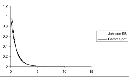
In this section we present several numerical examples. In these examples, we compare the probability distribution function of a number of variates that have known probability distributions (e.g., Beta and Gamma, etc.), with their approximations by Johnson

distribution, in order to validate this algorithm.

Example 1

In this example we fit Johnson distribution to Beta and Gamma distributions with various parameter values. To start the algorithm we need the first four moments of the variate. The first four moments of Beta and Gamma variates are given in [8] with respect to the parameters of each distribution. We take some cases of these variates with different values for their parameters, and use the values of their moments as input to the algorithm. After the algorithm determines the family type and evaluates the parameters of the

(22)

distribution and the actual probability density functions of Gamma and Beta are shown here.

0 0.2 0.4 0.6 0.8 1 1.2 1.4 1.6

0 1 2 3 4 5

x

f(x

) Johnson SB

Gamma pdf

Figure 2-6: Fitting Johnson distribution to Gamma with shape parameter =3 and scale parameter =5

0 0.2 0.4 0.6 0.8 1 1.2

0 5 10 15

Johnson SB Gamma pdf

(23)

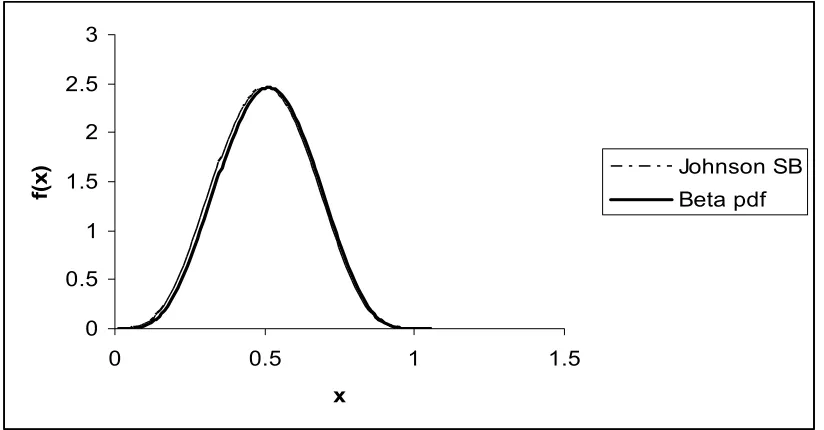
0 0.5 1 1.5 2 2.5 3 3.5 4

0 0.5 1 1.5

x

f(x)

Johnson SB Beta pdf

Figure 2-8: Fitting Johnson distribution to Beta with α=.5 andβ =.5

0 0.5 1 1.5 2 2.5 3

0 0.5 1 1.5

x

f(

x

) Johnson SB

Beta pdf

Figure 2-9: Fitting Johnson distribution to Beta with α =5 and β=5

(24)

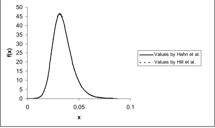
Example 2

In this example we solve a case that is originally presented in [8]. In this case the corresponding(β₁,β₂)point is in theS_U region. We find the parameters of Johnson S_U

family by the method that we discussed earlier and compare them with the results in [8]. In this example measurements of the coefficient of friction for a metal were obtained on 250 samples. The mean, standard deviation, the skewness and the peakedness are estimated from the sample and are presented in [8] as 0.0345 for mean, 0.0098 for variance, 0.87 for skewness and 4.92 for peakedness, respectively. Plotting the values of (0.87)2 0.7569

1 = =

β andβ₂ =4.92 in Figure 2-2 suggests the use of a Johnson S_U

distribution. Table 2-1 shows the values of the parameters that are found by each method.

Parameters of

U

S

Hahn and Shapiro

Hill, Hill and Hull

γ -1.783 -1.785

η 2.433 2.446

λ 0.0169 0.0169

ε 0.0198 0.0198

Table 2-1: Coefficient of Friction Example

(25)

0 5 10 15 20 25 30 35 40 45 50

0 0.05 0.1

x

f(

x

)

Values by Hahn et al. Values by Hill et al.

Figure 2-10: Comparison of methods

(26)

Chapter 3

Evaluating the First Four Moments of the Response Function

In this Chapter we discuss two methods for determining the moments of Y, where )

,..., (x₁ x_n h

Y = as described in Chapter 1. We assume that we know the probability density function for each component variablex₁,...,x_n. We further assume that the

function h is given in closed form and that it is continuous and differentiable at all points. Both methods that are discussed here are approximation methods, since determining the exact values of the moments of Y can be computationally difficult, if at all possible. One of these two methods is based on Monte-Carlo simulation and the other method is based on the Taylor series expansion of the function h.

3.1 Monte-Carlo Simulation

In this method with help of a computer program, capable of generating random numbers, we generate a value for each of the components x₁,...,x_nand determine the corresponding value of Y. If we repeat this process k times, we can create a collection of k

randomly generated values for Y (i.e., a random sample of Y).

Based on this random sample, we can estimate the first four moments of Y by a series of formulas that are adopted from [8].

1- Estimating mean:

k y y k i i

∑

=

= 1 _(3-1)

2- Estimating variance:

) 1 ( ) ( ) ( 1 1 2 2 1 2 2 2 ₋ − = − = =

∑

=

∑

=

∑

= k k y y k k y y m k i k i i i k i i

σ) (3-2)

(27)

3-Estimating the third moment: 3 1 1 1 2 1 3 1 3

3 3 2

) (             + − = − =

∑

=

∑

=

∑

=

∑

=

∑

= k y k y k y k y k y y m k i i k i i k i i k i i k

i i _(3-3)

4-Estimating the fourth moment:

4 1 1 2 2 1 1 3 1 1 4 1 4

4 4 6 3

) (             −             + − = − =

∑

=

∑

=

∑

=

∑

=

∑

=

∑

=

∑

= k y k y k y k y k y k y k y y m k i i k i i k i i k i i k i i k i i k

i i _(3-4)

Then the skewness of Y is estimated as

₃_/₂

2 3 1 ₍_m ₎

m

b = , (3-5)

and the peakedness of Y is estimated as

₂ 2 4 2 ) (m m

b = . (3-6)

Equations (3-1) and (3-2), i.e., y andm₂, can be used as estimates for mean and variance of Y respectively. Equations (3-5) and (3-6), i.e., b₁ andb₂, can be used to

estimate β₁ andβ₂, respectively.

3.2 Taylor Series Approximation

Tukey [14] develops a collection of formulas for approximating the first four moments of the random variate Y. These formulas are based on the Taylor series expansion of the function h about the pointµ₁,...,µ_n, using its first few terms.The complete forms of these formulas are given in [14], and we employ a simplified version of these formulas as given below. In these formulas the following notations are used for the moments of the

components (x_i,i=1,2,...,n): mean of x_i=µ_i, variance of x_i= 2 i

(28)

and peakedness of x_i=Γ_i. Also µ_Y denotes the mean of Y, 2 Y

σ denotes the variance of Y,

Y

φ denotes the third central moment of Y about its mean, and ϕ_Y_{denotes the fourth} central moment of Y about its mean.

) ,..., ,

( 1 2 n

Y h µ µ µ

µ ≈ . (3-7)

2 2 2 i i i

Y h σ

σ ≈

∑

(3-8)

3 3

i i i i

Y h γ σ

φ ≈

∑

(3-9)

4 4 4₍ ₃₎ ₃

Y i i i i

Y h σ σ

ϕ ≈

∑

Γ − + (3-10)

In these formulas all the summations are form 1 to n, and

n i i _x h h µ µ µ, 2,..., ∂

∂

= .

Formulas for more accurate approximation of these parameters are presented in [14]. These formulas contain higher order terms of the Taylor series approximation.

3.3Numerical Examples

In this section we present two numerical examples and observe the accuracy of these two methods for determining the moments of Y. In example 1, we only use the Monte-Carlo simulation method since the corresponding function is linear, and in example 2 we use both methods.

Example 1

We consider the following function: y=x₁+x₂+x₃, and we assume ~ (2,12),

1 N x ), 1 , 3 ( ~ 2 2 N

x and ~ (5,22)

3 N

x .

Of course in this example it is easy to determine the exact form of the probability distribution function of y and its parameters. It is clear that y has a normal distribution with the following parameters: mean of y is µy = 2+3+5=10, variance of y is

=

2 y

σ 12 ₊12₊22 ₌6_{. Skewness and peakedness of}_y_{are 0 and 3, respectively since}_y_is

(29)

In order to evaluate these parameters using the Monte-Carlo simulation method, we randomly generate 250,000 values for each component. Then we determine the

corresponding values for the function y. We can then estimate mean, variance, skweness and peakedness of y using equations (3-1) through (3-6). Table 3-1 shows the results from simulating this function versus the values that are calculated analytically.

Parameter Values form

Simulation Actual Values

Mean 10.0090 10

Variance 6.0034 6

Skewness 0.0018 0

Peakedness 2.9953 3

Table 3-1: Comparing the results form simulation with actual values

As it is observed, the results are very close to the actual moments. The 95% confidence interval for mean in this example is [9.9993, 10.0186] and for variance is

[5.9703, 6.0369].

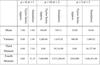
Example 2

We consider the function _y₌_x2_{and assume that}_x_~ _N₍_µ_,_σ2₎_{. In this example we}

(30)

1 ,

0 =

= σ

µ µ =10,σ =2 µ =5,σ =3

Taylor Series

Approx. Simula

tion

Taylor Series

Approx. Simula

tion

Taylor Series

Approx. Simula

tion

Mean 1.00 1.00 104.00 104.11 34.00 34.60

Variance 0.00 1.98 1,600.00 1,639.20 900.00 1,086.82

Third

Moment 0.00 7.50 0.00 39,314.00 0.00 56,757.00

Fourth

Moment 0.00 51.53 7,680,000 9,313,200.00 2430,000 7,446,421.00

Table 3-2: Comparing Taylor approximation method with Monte-Carlo simulation

Comparison shows that Taylor series approximation method approximates mean and variance of the variate relatively well. However, it is observed that the approximated values for the third and the fourth moments of yare quite inaccurate. In this example we deliberately choose a simple function (_y₌_x2_{) to show that Taylor series approximation}

(31)

Chapter 4 Methodology

In this Chapter we propose a methodology for developing an interactive model for the Parameter Design Problem, as defined in Chapter 1. We also discuss a computer program that we have developed for this interactive model and present a numerical example.

4.1 The Model

In the context of the Parameter Design Problem as we defined earlier, we need to determine a set of values for the controllable parameters, µ₁,...,µ_nso that the

corresponding value of the response variable, Y, is at or close to its target valueτ , with minimum variation. To this end we propose an interactive model and a corresponding computer program, in which the user is able to graphically observe the probability distribution of Y for a given set of values forµ₁,...,µ_n. We then allow the user to change the values of one or more of the parameters (i.e., µ₁,...,µ_n) and immediately observe the impact of this change on the graph of the corresponding probability distribution of Y. In this model the user can make a subjective assessment of the distribution of Y by

comparing it with its target value and its specification limits. Objective measurements such as the corresponding values of the “percent defective” or the “expected loss

function” can also be estimated to assist the user in evaluating the quality of the solution. In this manner the user can employ this interactive model to determine an appropriate set of values forµ₁,...,µ_n.

(32)

Step 1-Approximating the First Four Moments of Y

In Chapter 3 we discuss two methods for approximating the moments of a distribution, i.e., Monte-Carlo simulation and Taylor series approximation. Monte-Carlo simulation is more accurate but more time consuming. Taylor series approximation is less accurate in this case but obviously much faster. In this model we approximate the first four moments of the random variate, Y, with one of these two methods, as appropriate. See Remark 1 below.

Step 2- Fitting Johnson Distribution

After approximating the first four moments of Y, we can use the numerical methods of Hill et al. [9] to find the corresponding Johnson family, as we discuss in Chapter 2. Once the parameters of the Johnson distribution are known, we can form the pdf of the

response function, using equations (2-6) through (2-8), and plot it. This pdf can be used to calculate different measures of variation such as estimating the “fraction defective” or the “expected loss function”. Evaluation of these measures can be saved for further comparison with other feasible combinations of set points. We can also provide assistance to the user for determining an appropriate set of values forµ₁,...,µ_n. To this end we can employ a non-linear programming model as discusses in [7] or use other techniques.

Remark 1

(33)

while changing the values ofµ₁,...,µ_n, we assume that the values of the third and the fourth moments of Y remain unchanged; we use Taylor series method to approximate the first two moments of Y during the interactive phase and carry out the analysis

accordingly. When the interactive phase is complete, once again we employ a Monte-Carlo simulation model to approximate the third and the fourth moments. If their values at this stage are significantly different from their values at the start of the interactive phase, we update their values and repeat the interactive phase. If, on the other hand, their terminal values are reasonably close to their original values, we terminate the procedure.

Remark 2

As a terminating criterion we use the corresponding value of the fraction defective as estimated by using the fitted Johnson distribution. First we evaluate the fraction defective at the original set points, and refer to it asp₀. In the interactive phase we try to reduce the value of the fraction defective by changing the values of the set points. Then we evaluate the fraction defective at the end of the interactive phase via the fitted Johnson

distribution, using its mean and variance as calculated by Taylor series approximation and its skewness and peakedness as the initial values obtained via Monte-Carlo simulation at the start of the interactive phase. We refer to this value asp₁.

Now we employ a Monte-Carlo simulation model to re-evaluate the moments of the response at the current set points. Then we calculate the fraction defective with these updated values of the moments. We refer to this value asp₂. If p₁and p₂are sufficiently close to each other we terminate the algorithm. Otherwise we repeat the interactive phase using the updated values of the third and the fourth moments.

(34)

(35)

4.2 Computer Program

We have developed a computer program to implement this interactive approach for the Parameter Design Problem. Microsoft Excel with VBA in its background is chosen to develop this model. There are two main reasons for this choice: the high graphical capability of MS Excel to draw plots and charts, and availability of the software on almost every desktop. Since in this method the graphs for the pdf should be plotted every time that the set points are changed, visual features of MS Excel charts make it relatively easy to carry out this approach. Appearance of charts can be edited to the user’s taste and other features can be added as the user wishes. Another reason that makes MS Excel appealing in this context is the fact that it is available on almost any machine in work environments and the users have easy access to the software. Therefore, potential users do not need to install a new software package on their machines.

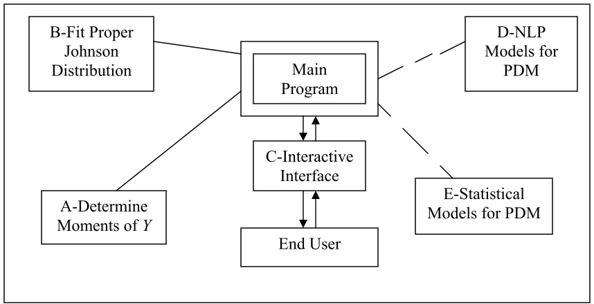
4.2.1 Modules of the Program

(36)

``

Figure 4-2: Schematic view of the program

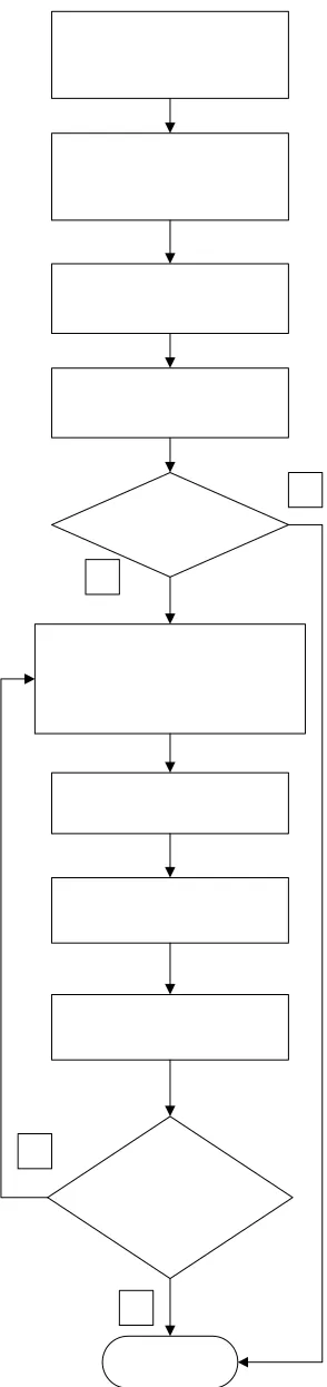
Procedure A that is designed to approximate the first four moments of the response function, takes the closed form relationship between the response function Y and the components as well as the first four moments of the components as input. This program is designed such that a response function with up to ten arguments can be given as input. Once the input is entered in the designated worksheet (this worksheet is called “Moments of Y”), a macro which is called “FunctionMom” will approximate the first four moments of Y as well as its skewness and peakedness using the Taylor series approximation method. For the Taylor series approximation method we use the formulas of Chapter 3, i.e., (3-7) through (3-10).

To evaluate the partial derivatives in these formulas, we use the symmetric difference quotient formula for numerical approximation of first derivative which is

δ δ

δ

2

) ( ) ( ) (

' _x ₌ f x+ − f x−

f (4-5).

Here, δ represents incremental changes in variable x, and Evans [5] recommends usingδ =σ in the context of the above formulas.

From this point, the next part of the methodology, i.e., fitting Johnson distribution, begins and all of the calculations for this part are done by a macro that is called

“JOHNSONTYPES”. This macro copies the mean, variance, skewness and peakedness of the response, from the Table in the worksheet “Moments of Y”, to a designated Table in

B-Fit Proper Johnson

Distribution Main

Program

D-NLP Models for

PDM

A-Determine Moments of Y

E-Statistical Models for PDM C-Interactive

Interface

(37)

another worksheet that is called “Johnson”. First the macro checks if there are any flaws in the input to this step. To this end location of (β₁,β₂) is checked against Figure 2-2 to determine if the point is in the impossible area. If this point is in the impossible area, message “IMPOSSIBLE AREA” will appear as an indication of system failure.

Otherwise, the standard deviation is checked for non-negativity. If both of the tests are passed, then a message will appear to show that the input is successfully entered. In this case, the program proceeds to determine the type of the Johnson family by methods that are discussed in Chapter 2. There will be five possible outputs from this stage, namelyS_U,S_B,S_L,S_T, and Normal. Once the type is determined, the macro begins its procedure to approximate the parameters of the respective type. If the Johnson

families S_U orS_B are chosen, the program calls the corresponding subroutines for S_U or

B

S respectively. In the case ofS_L, Normal,andS_T families, the corresponding procedures are in the main body of the macro “JOHNSONTYPES”. After estimating the parameters of the Johnson distribution as appropriate, the parameters are inserted in a designated tablein the worksheet “Johnson”.

At this time the last main macro is called. This macro plots the probability distribution function of the response, Y, as well as the specification limits on a graph.

Now the user can start trying different set points for the components. He or she can see the effect of the change on the distribution of the response for each combination of the set points. The complete script of this program is presented in Appendix 2. Figures (4-3) and (4-4) show a view of worksheets “Moments of Y” and “Johnson” for a numerical

example. We include these snapshots of the screen in order to offer a view of the interactive environment, and the numerical values are not meant to correspond to any specific example that we describe here.

(38)

Cells A15, A23 and A31 show the values of the partial derivatives with respect

tox₁,x₂andx₃ for this example, respectively. Then the estimated values of the mean, the standard deviation the third moment and the fourth moment of Y are calculated in cells N9 through N12, via formulas of Chapter 3. At the end, the skewness and the peakedness of Y are evaluated in cells N13 and N14 from the values of its moments.

(39)

Figure 4-4: View of “Johnson” worksheet

4.3 A Numerical Example

Consider an output characteristic, Y, which is a function of three components

2 1,X

X andX₃. The response function is given as 2 ₃ 2 2

1 3 )

(X X X

Y = + . Suppose

2 1,X

X and X₃ are normally distributed random variables with respective means

2 1,µ

µ andµ₃, and standard deviations σ₁ =0.1,σ₂ =0.1andσ₃ =0.01. Specification limits for Y are, 3,255 ±150. The following are the technical constraints on

2 1,µ

(40)

20 10

10 2

3 2 1

≤ ≤

µ µ µ

We start with the following combination of set points: µ₁ =5,µ₂ =8 andµ₃ =15. Table 4-1 shows the approximated values of the mean, variance, skewness and

peakedness of Y at these set points by Monte Carlo simulation.

Mean 3,255.6 Standard Deviation 73.479

Skewness 0.036404 Peakedness 2.9941

Table 4-1: Results of MC simulation at the initial set points

The program approximates the distribution of this function to be JohnsonS_L. The fraction defective at this combination is approximately p0 =3.45%. Figure 4-5 shows the

graph of probability density function of Y.

PDF AND LIMITS

0 0.001 0.002 0.003 0.004 0.005 0.006

2900 3000 3100 3200 3300 3400 3500 3600 3700

X

F(

X

) PDF

LSL USL

(41)

We now start the interactive phase of the program and after trying a number of combinations of set points for µ₁,µ₂,andµ₃, we find the combination µ₁ =7.34,

0935 . 8

2 =

µ andµ₃ =13 to be a better combination than the first one. For this

combination Table 4-2 shows the approximated values of the mean, variance, skewness and peakedness of Y at the new set points. Note that the mean and variance are calculated by Taylor series method and skewness and peakedness are from the Monte-Carlo

simulation at the starting combination (i.e., at the start of the interactive phase).

Mean 3,255.0677 Standard Deviation 65.9983

Table 4-2: Results of MC simulation at the new set points

The program approximates the distribution of this function as JohnsonS_L too. The corresponding value of the fraction defective for this combination is p1 =2.32%.

Figure 4-6 shows the graph of probability density function of Y.

PDF AND LIMITS

0 0.001 0.002 0.003 0.004 0.005 0.006 0.007

2900 3000 3100 3200 3300 3400 3500 3600 3700

X

F(

X

) PDF

LSL USL

(42)

Now we simulate the response function with this combination of set points by Monte-Carlo simulation, and compare its first four moments with the values of Table 4-2. Table 4-3 shows the results from simulation.

Mean 3255.03 Standard Deviation 65.921

Table 4-3: Results of MC simulation at the final stage

The fraction defective here is p₂ =2.32%. Figure 4-7 shows the probability density function of this combination with moments estimated by Monte-Carlo simulation, which of course closely resembles Figure 4-6.

PDF AND LIMITS

0 0.001 0.002 0.003 0.004 0.005 0.006 0.007

2900 3000 3100 3200 3300 3400 3500 3600 3700

X

F(

X

) PDF

LSL USL

Figure 4-7: Pdf of Y with new set points, moments estimated by MC simulation

(43)

(44)

Chapter 5 Case Studies

In this Chapter we present two case studies to illustrate the interactive model and the corresponding software, for the Parameter Design Problem. Throughout this Chapter all the assumptions of Chapter 1 for Parameter Design Problem hold. In each case we start with the original set points of the components and then find other set points that decrease the variation of the response function while keeping its nominal value on target. The final results are then verified with Monte-Carlo Simulation.

5.1 Deflection of a Coil Spring 5.1.1 Statement of the Problem

We have adopted this example from [6] and applied some changes to it. A detailed description of the problem can be found in [6]. Let δ denote the deflection along the axis of the spring. As discussed in [6] deflection,δ , is a function of three components, wire diameter, d, coil diameter, D, and number of active coils, N. The relationship is given as: 3 ₄ 143750d N D = δ

We assume that each component is a normally distributed random variable with given values of its mean and standard deviation as below:

), 00174 ,. 0517 (.

~ _N 2

d ), 0197 ,. 357 . 0 (

~ _N 2

D ) 185 ,. 29 . 11 ( ~ 2 N .

The technical requirements on the set points of the components are:

30 . 1 25 . 0 20 . 0 05 . 0 ≤ ≤ ≤ ≤ D d µ µ 15 2≤µN ≤

(45)

5.1.2 Distribution of δat the Original Set Points

We use the given values for the mean and the standard deviation of the components, and values 0 and 3 for their skewness and peakedness (the components are all normal variates). A Monte-Carlo Simulation of this function with the original set points gives the following results in Table 5-1.

Mean 0.51037

Standard Deviation 0.10995

Table 5-1: Results from Monte-Carlo Simulation at the initial set points

When these values are fed to the procedure for Johnson fitting, the result is an

L

S distribution. The corresponding value of the fraction defective isp0 =34.64%.

Figure 5-1 shows the plot for this pdf. In this plot the target value of δ (0.5 in) and its specification limits (LSL=0.4 and USL=0.6) are clearly marked.

PDF AND LIMITS FOR SPRING DEFLECTION

0 0.5 1 1.5 2 2.5 3 3.5 4 4.5

0 0.5 1 1.5 2

X

F(

X

)

USL _LSL

TARGET VALUE

(46)

From Figure 5-1 we observe that the original set points for the components make the mean of the response function slightly off target (i.e., not exactly equal to 0.5 in). We also observe that there is a relatively high probability for deflection of the spring to violate its specification limits, as reflected in the corresponding value of the fraction defective. Histogram of the data set from Monte-Carlo simulation is shown in Figure 5-2 for comparison.

0 100 200 300 400 500 600 700

0.19 654

0.34 409

6962

0.491 6539

24

0.63 9210

886

0.78 67678

48

0.9343 2481

1.08 1881

772

Bin

Fr

e

quenc

y

Figure 5-2: Histogram at the original set points.

5.1.3 Interactive Stage

(47)

component. If the partial derivative with respect to a specific component is positive, it implies that increasing the value of that component results in an increase in the mean value of Y and if the partial derivative is negative, increasing the value of that component results in a decrease in the mean value of Y.

Table 5-3 shows some of the different combinations of set points that we tried, in decreasing order of their respective values of fraction defective. In this table we only present those combinations of the set points that satisfy the technical constraints and result inµ_δ ≈0.5. We tried many other combinations of values forµ_d,µ_D, and µ_N in the context of designing the parameters interactively.

Set Points Response

d

µ µD µN µδ σδ

Skewness Peakedness

Johnson Type Fraction Defectiv

e

0.05640 0.4826 6.460 0.49919 0.08818 0.5929 3.631 SL 24.61%

0.05642 0.4826 6.467 0.49903 0.08814 0.5929 3.631 SL 24.60%

0.06081 0.6200 4.110 0.49832 0.07772 0.5929 3.631 SL 18.73%

0.06500 0.7474 3.067 0.49901 0.07307 0.5929 3.631 SL 15.99%

0.07598 0.8796 3.514 0.49917 0.06259 0.5929 3.631 SL 9.99%

0.13660 1.3000 11.360 0.49865 0.03502 0.5929 3.631 SL 0.80%

Table 5-2: Improvement of fraction defective for spring deflection

Some of the combinations in this table are suggested in Table 2 of [6]. Note that for all

of the combinations in Table 5-2, we use the same skewness and peakedness that we found for the original combination, via Monte-Carlo simulation presented in Table 5-1 (i.e., skewness = 0.5929 and peakedness = 3.631). Figure 5-3 shows the probability density function of deflection at the best combination of set points, i.e., µ_d =0.1366,

3 . 1

=

D

(48)

simulation of the original combination. The value of the fraction defective at this combination of set points isp1 =0.80%.

PDF AND LIMITS FOR SPRING DEFLECTION

0 2 4 6 8 10 12 14

0 0.5 1

X

F(

X

)

USL LSL

Figure 5-3: Best case with skewness and peakedness of the starting point

Now as it is explained in Chapter 4, we calculate the moments of the response function at this best combination, by Monte Carlo simulation. Table 5-3 shows the values from Monte-Carlo simulation.

Mean 0.49986

Table 5-3: Results from MC simulation for the best case in Table 5-2

The program fits a Johnson S_B distribution using the moments in Table 5-3. The fraction defective for this distribution is p2 =0.48 %. Figure 5-4 shows the pdf of this

(49)

0 2 4 6 8 10 12

0 0.2 0.4 0.6 0.8 1

X

F(X

)

Figure 5-4: Best Case Found by Interactive Model with moments from Monte-Carlo simulation

The fraction defectivep₂= 0.48%, calculated with moments from Monte-Carlo

simulation, is not sufficiently close to p1 =0.80% (more than 5% which is our limiting

(50)

Set Points Response

d

µ µD µN µδ σδ

Skewness Peakedness

Johnson Type Fraction Def

ectiv

e

0.1360 1.34 10.3 0.50395 0.03524 0.21865 3.0723 SB 0.59%

0.1365 1.35 10.2 0.50288 0.03502 0.21865 3.0723 SB 0.52%

0.1365 1.40 9.1 0.50036 0.03466 0.21865 3.0723 SB 0.43%

Table 5-4: Improvement of fraction defective in spring deflection with a new starting point

As it is shown in this table, the last combination results in the least fraction defective compared to other combinations that we have tried. The corresponding value of fraction defective at this combination is p₁= 0.43%. Figure 5-5 shows the probability density function for this combination.

0 2 4 6 8 10 12

0 0.5 1

X

F(

X

)

(51)

Monte-Carlo simulation for this combination gives the following results:

Mean 0.50146

It is observed that the skewness and peakedness from the Monte-Carlo simulation are relatively close to the skewness and peakedness of the new starting point. The

corresponding value of the fraction defective is p₂= 0.45%. Since this value is within 5% of the value ofp₁, we can stop here and keep this combination as an acceptable solution.

5.2 An Output Transformerless Pull-Push Circuit 5.2.1 Statement of the Problem

This example deals with an Output Transformerless (OTL) Pull-Push Circuit. A graphical representation of this circuit is given in Figure 5-6. We have adopted this example form [6] with slight modifications.

2

b

R

1

b

V

1

b

R

1

b

R

L

R Rc2

f

R

1

c

R

m

V

c

E

+

β

4

β

3

β

1

β

(52)

The performance characteristic of interest is V_m and the response function is given by 1 2 3 1 1 ) ( ) ( ) ( c f f be f f be c f be b m R R R R R V R R R V E R R R V V V + + + − + + + = o o o o o β β β β β where 2 1 2 1 b b b c b R R R E V +

= and Ro =R_c2 +R_L

with R_L =9Ohms,Vbe₁ =Vbe₃ =0.65 Volts, 74Vbe2 =0. Volts, and Ec =12 Volts.

, , ,

, ₁ ₂

2 b f c

b R R R

R and R_c₁ are resistances, and β is the current gain of the transistor. The means of these components are denoted byµ₁through µ₆ and standard deviations are denoted byσ₁ throughσ₆, respectively. Parameters µ₁through µ₆ are controllable. All the components are assumed to be normally distributed. The technical requirements of

1

µ through µ₆ are as below:

70000 25000≤µ₁ ≤

150000 50000≤µ₂ ≤

5 . 2053 4

.

649 ≤µ₃ ≤

9 . 749 1

.

237 ≤µ₄ ≤

3 . 2260 1

.

1271 ≤µ₅ ≤

280 73≤µ₆ ≤

Target value for V_m is 6 Volts. We further assume that the specification limits for V_m are6±0.2.

The original set points and the standard deviations of the components are given as below. , 1271 , 1 . 237 , 2054 , 117100 ,

48930 ₂ ₃ ₄ ₅

1 = µ = µ = µ = µ =

µ and µ₆ =73

i

i µ

σ =0.02 for i=1,...,5, and σ₆ =0.15µ₆.

5.2.2 Variation with the Original Set Points

(53)

normality), Monte-Carlo simulation gives the values for the mean, standard deviation, skweness and peakedness of V_m as in Table 5-5.

Mean 6.0073

Table 5-5: Results from Monte-Carlo Simulation for the original set points

When the distribution of V_m is approximated with a Johnson distribution through our model, the resulting pdf is JohnsonS_U. Figure 5-7 shows this pdf.

PDF AND LIMITS FOR OTL PUSH PULL CIRCUIT

0 0.5 1 1.5 2 2.5 3 3.5 4

5 6 7

X

F(

X

)

LSL USL

TARGET VALUE

Figure 5-7: OTL Circuit with original set points

We observe that the mean of V_mis very close to its target value (i.e.,µV_m ≈6) but the probability that V_m violates its specification limits is considerably high. The

(54)

0 100 200 300 400 500 600

0.21112 0.34

34427 85

0.4757655 7

0.60 80883

54

0.74 04111

39

0.87 27339

24

1.00 50567

09

Bin

Fr

equency

Figure 5-8: Histogram at the original set points.

5.2.3 Interactive Stage

(55)

Set Points Response

1

µ µ2 µ3 µ4 µ5 µ6

Mean

Standard Deviation

Skewness Peakedness

Johnson Types Fraction Defectiv

e

56500 87000 1044 500 1275 280 6.0197 0.08255 0.4208 3.6557 S_U 2.54

%

55000 85000 1044 500 1275 280 6.0093 0.08249 0.4208 3.6557 S_U 2.17

%

55835 75000 649.4 749.9 2260.3 280 6.0000 0.08306 0.4208 3.6557 S_U 2.00

%

56590 87010 1044 746.2 1302 280 5.9987 0.0825 0.4208 3.6557 S_U 1.92

%

58750 100000 1539.9 237.1 1467.8 280 5.9871 0.0828 0.4208 3.6557 S_U 1.76

%

Table 5-6: Improvement in fraction defective

In this table, the best combination of set points appears in the last row, i.e.,µ₁ =58750,

, 8 . 1467 ,

1 . 237 ,

9 . 1539 ,

100000 ₃ ₄ ₅

2 = µ = µ = µ =

µ andµ₆ =280. The corresponding

value of the fraction defective is p₁ = 1.76%.

Now we conduct a Monte-Carlo simulation with the set points of the best case combination. Table 5-7 shows the results and Figure 5-9 shows the fitted Johnson

B

S distribution.

Mean 6.011

(56)

PDF AND LIMITS FOR OTL CIRCUIT

-1 0 1 2 3 4 5

5.5 5.7 5.9 6.1 6.3 6.5

X

F(

X

)

Figure 5-9: Fitted Johnson distribution of the best case set points.

The corresponding values of the fraction defective for this distribution is p₂ = 1.65%. Since the value p₂is not within 5% ofp₁, we resume the interactive stage with updated values of the skewness and peakedness as 0.02016 and 2.9879, respectively. We use this combination as a new starting point and resume trying different combinations. Table 5-8 shows the results of this trial.

Set Points Response

1

µ µ2 µ3 µ4 µ5 µ6

Mean Deviation Standard Skewness

Peakedness

Johnson Types Fraction Defectiv

e

55500 85500 1044 500 1275 280 6.0184 0.08255 0.02016 2.9879 S_B 1.78%

55000 85500 1044 500 1275 280 5.9927 0.08239 0.02016 2.9879

B

S 1.54%

55500 85000 1044 600 1350 280 5.9953 0.08246 0.02016 2.9879 S_B 1.52%

(57)

In Table 5-8, the combinations are sorted in decreasing order of their fraction defective. As before, the skewness and peakedness from the Monte-Carlo simulation of the new starting combination (i.e., from Table 5-7) are used as the skewness and the peakedness at all combinations. The combination with the least fraction defective is the combination at the last row of Table 5-8, with value of p1 =1.51%

Now we conduct a Monte-Carlo simulation with the last combination in this table. The results are shown in Table 5-9.

Mean 5.994

Table 5-9: Results from Monte-Carlo simulation of the best case

We can observe that the values of skewness and peakedness by Monte-Carlo simulation are reasonably close to the values in Table 5-7 for the best case combination. The