Inference on some epidemiological indices and variance function in semi-parametric analysis of count data

(1)

University of Windsor University of Windsor

Scholarship at UWindsor

Electronic Theses and Dissertations Theses, Dissertations, and Major Papers

2009

Inference on some epidemiological indices and variance function

in semi-parametric analysis of count data

Tasneem Zaihra

University of Windsor

Follow this and additional works at: https://scholar.uwindsor.ca/etd

Recommended Citation Recommended Citation

Zaihra, Tasneem, "Inference on some epidemiological indices and variance function in semi-parametric analysis of count data" (2009). Electronic Theses and Dissertations. 7888.

https://scholar.uwindsor.ca/etd/7888

This online database contains the full-text of PhD dissertations and Masters’ theses of University of Windsor students from 1954 forward. These documents are made available for personal study and research purposes only, in accordance with the Canadian Copyright Act and the Creative Commons license—CC BY-NC-ND (Attribution, Non-Commercial, No Derivative Works). Under this license, works must always be attributed to the copyright holder (original author), cannot be used for any commercial purposes, and may not be altered. Any other use would require the permission of the copyright holder. Students may inquire about withdrawing their dissertation and/or thesis from this database. For additional inquiries, please contact the repository administrator via email

(2)

I N F E R E N C E ON SOME E P I D E M I O L O G I C A L INDICES

AND V A R I A N C E F U N C T I O N

IN SEMI-PARAMETRIC ANALYSIS O F COUNT DATA

by

Tasneem Zaihra

>

A Dissertation

Submitted to the Faculty of Graduate Studies

through the Department of Mathematics and Statistics

in Partial Fulfillment of the Requirements for

the Degree of Doctor of Philosophy at the

University of Windsor

Windsor, Ontario, Canada

2009

(3)

**1*1**

Library and Archives Canada

Published Heritage Branch

395 Wellington Street Ottawa ON K1A 0N4 Canada

Bibliotheque et Archives Canada Direction du

Patrimoine de I'edition 395, rue Wellington OttawaONK1A0N4 Canada

Your file Votre reference ISBN: 978-0-494-57658-8 Our file Notre r6f6rence ISBN: 978-0-494-57658-8

NOTICE: AVIS:

The author has granted a

non-exclusive license allowing Library and Archives Canada to reproduce,

publish, archive, preserve, conserve, communicate to the public by

telecommunication or on the Internet, loan, distribute and sell theses

worldwide, for commercial or non-commercial purposes, in microform, paper, electronic and/or any other formats.

L'auteur a accorde une licence non exclusive permettant a la Bibliotheque et Archives Canada de reproduire, publier, archiver, sauvegarder, conserver, transmettre au public par telecommunication ou par I'lntemet, prefer, distribuer et vendre des theses partout dans le monde, a des fins commerciales ou autres, sur support microforme, papier, electronique et/ou autres formats.

The author retains copyright ownership and moral rights in this thesis. Neither the thesis nor substantial extracts from it may be printed or otherwise reproduced without the author's permission.

L'auteur conserve la propriete du droit d'auteur et des droits moraux qui protege cette these. Ni la these ni des extraits substantiels de celle-ci ne doivent etre imprimes ou autrement

reproduits sans son autorisation.

In compliance with the Canadian Privacy Act some supporting forms may have been removed from this thesis.

Conformement a la loi canadienne sur la protection de la vie privee, quelques

formulaires secondaires ont ete enleves de cette these.

While these forms may be included in the document page count, their removal does not represent any loss of content from the thesis.

Bien que ces formulaires aient inclus dans la pagination, il n'y aura aucun contenu manquant.

1+1

(4)

Declaration of Previous Publication

This dissertation includes an original paper [Chapter 3, p. 17-40] that has been previously

published in a peer reviewed journal, as follows:

Thesis Chapter

Chapter 3

Citation

Paul S.R. and Zaihra T. (2008). Interval estimation

of risk difference for data sampled from clusters.

Statistics in Medicine, 27: 4207-4220.

Publication status

Published

I certify that I have obtained written permission from the copyright owner to include the

above published material in my dissertation (a copy of permission is attached in Appendix

A.5). I certify that the above material describes work completed during my registration as

a graduate student at the University of Windsor.

I declare that, to the best of my knowledge, my dissertation does not infringe upon

any-one's copyright nor violate any proprietary rights and that any ideas, techniques, quotations,

or any other materials from the work of other people included in my dissertation, published

or otherwise, are fully acknowledged in accordance with standard referencing practices.

Fur-thermore, to the extent that I have included copyrighted material that surpasses the bounds

of fair dealing within the meaning of the Canada Copyright Act, I certify that I have obtained

written permission from the copyright owner to include such materials in my dissertation.

I declare that this is a true copy of my dissertation, including any final revisions, as

approved by my committee and the Graduate Studies Office, and that this dissertation has

(5)

Abstract

Clustered binary data arise in many fields such as epidemiology, toxicology, econometrics

and pharmacokinetics modelling. For instance, in many epidemiological studies the purpose

of the investigation is to compare the risk experienced between two groups where each

group has clustered observations. Several methods have been developed in the literature for

interval estimation of epidemiological indices such as the risk difference, the risk ratio and

the relative difference. In this dissertation we introduce two very simple methods. One of

these is based on an estimator of the variance of a ratio estimator and the other is based

on a sandwich estimator of the variance of the regression estimator using the generalized

estimating equations (GEE) approach. We then compare these two methods, by simulation,

in terms of maintaining nominal coverage probability and average coverage length, with the

four methods discussed earlier in the literature. It is shown that the methods based on an

estimator of the variance of ratio estimate performs better in terms of coverage probability,

symmetry and bias. The proposed methods are then applied to analyze toxicological and

educational intervention program datasets.

The phenomenon of overdispersion is also quite common in count data. Overdispersion

is suspected when the variance is larger than the mean. In semi-parametric analysis of

overdispersed count data, one often needs to determine an appropriate variance function

(mean variance relationship). For example, in chemical and biological assay problems, to

control the quality of techniques, one has to adjust the levels of experimental factors to

bring the mean response to a target value while minimizing variance. The emphasis is on

(6)

may be a function of the former. In this dissertation, by using a hypothesis testing approach

through a broader class of models and a data analytic approach, we propose an appropriate

(7)

Dedication

(8)

A c k n o w l e d g e m e n t s

My most heartfelt appreciation goes to my supervisor. Dr. Sudhir Paul. His vast

exper-tise, availability for help and guidance, his encouragement and patience were instrumental

in completion of this dissertation. His motivational spirit of academic research, financial

support throughout my research and assistance in tracking down errors and omissions made

it possible for me to finish this work on time.

I am extremely grateful to my doctoral committee members Dr. S. Paul, Dr. M. Hlynka,

Dr. R. Barron and Dr. J. Ciborowski for their constructive comments and criticism which

improved the presentation of this dissertation a great deal.

I can not do justice with mere words to the depth of gratitude I have towards my family

for their understanding, love and constant support. Special thanks to my parents,

parents-in-law, sister-parents-in-law, brothers-parents-in-law, my uncles Dr. Fazal Mehdi, Dr. Subodh Bhatnagar

and my aunts Dr. Neerja Bhatnagar, Dr. Alka Yadu and Dr. Alveera Mehdi. I would also

like to thank my sister Naseem Zaihra and my best friends Anshu and Swati who have been

far above and beyond the call of duty.

Finally I would like to thank the two most important men in my life, my brother Yasir

and my husband Hasan. I feel blessed to have Yasir in my life for all life enriching experiences

that we have gone through together. The understanding and support of my husband, his

phone calls, e-mails and patient tolerance of my sometimes hysterical whining, have been a

lifeline for me. I am so blessed to have him by my side and eagerly look forward to a lifetime

of togetherness. During my stay at University of Windsor, I had the opportunity to meet

(9)

talks with Dr.Barron, Dr. Chandna, Dr. Fling, Dr. Caron, Dr. Hussein, Dr. Ahmed and

Dr. Lau and all other faculty members made the day-to-day travail enjoyable. I acknowledge

my debt to all of them for their affectionate concern about my work and well being.

The research of this dissertation was further supported by the Ontario Graduate

arship in Science and Technology (OGSST), University of Windsor Doctoral Tuition

Schol-arships and graduate assistantships provided by Department of Mathematics and Statistics,

(10)

ist of Figures

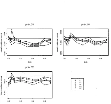
3.1 Bias of the 5 confidence intervals £1(0), £3(+), L4(x), C2(®) and 52(A) in

case of cluster size configuration (a). 34 3.2 Bias of the 5 confidence intervals L1(0), LS(+), L4(x), C2(«) and 52(A) in

case of cluster size configuration (b) 35 3.3 Bias of the 5 confidence intervals L1(0), £3(+), L4(x), C2(.) and 52(A) in

case of cluster size configuration (c) 36 3.4 Bias of the 5 confidence intervals £ 1 ( 0 ) , L3(+), I 4 ( x ) , C2(») and 52(A) in

case of cluster size configuration (d) 37

4.1 Bias of the confidence intervals of the three versions Ml, MR1 and MSI of

method 1 60 4.2 Bias of the confidence intervals of the three versions M2, MR2 and MS2 of

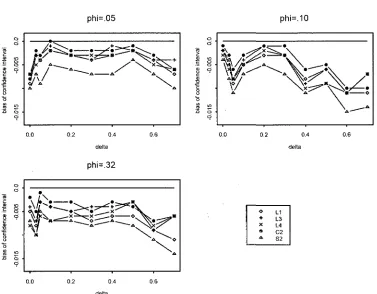
method 4 63 4.5 Bias of the confidence intervals by all four methods MR1, MR2, MR3 and

(15)

ist of Tables

3.1 Radiation exposure data. (Mayer et a l , 1997). (i) Class sizes, (ii) Observed

number of children with an inadequate level of solar protection 25 3.2 lexicological data. (Paul, 1982). (i) Number of live fetuses affected by

treat-ment, (ii) Total number of live fetuses 25 3.3 Coverage probabilities, average lengths of confidence intervals for the risk

difference A by the methods LI, L3, LA, (72, 52; equal number of clusters

m = n0 = 29 in both groups; TT0 = 0.20, (j) = 0.05; a = 0.05; based on 10,000

simulations 26 3.4 Coverage probabilities, average lengths of confidence intervals, for the risk

difference A by the methods LI, L3, LA, C2, 52; equal number of clusters

rii = n0 = 29 in both groups; TT0 = 0.20, <fi = 0.10; a = 0.05; based on 10,000

simulations 27 3.5 Coverage probabilities, average lengths of confidence intervals, for the risk

difference A by the methods LI. L3, LA, C2, 52; equal number of clusters rii = n0 = 29 in both groups; w0 = 0.20, (p = 0.32; a = 0.05; based on 10,000

simulations 28 3.6 Non-coverage probability ((left)(right)) for the risk difference A by the

meth-ods LI, L3, LA, C2, 52; equal number of clusters rii = no = 29 in both

(16)

3.7 Coverage probabilities and average lengths of confidence intervals, for the risk difference A by the methods LI, L3, LA, C2, 5*2; equal number of clusters

m = n0 = 29 in both groups: TT0 = 0.20, <p0 = 0.324, fa = 0.249; a = 0.05;

based on 10.000 simulations 30 3.8 Coverage probabilities, average lengths of confidence intervals for the risk

difference A by the methods LI, LZ, LA, C2, S2: equal number of clusters

n\ = no — 29 in both groups; 7r0 = 0.20, e6 = 0.8; a = 0.05; based on 10,000

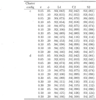
simulations 31 3.9 Coverage probabilities and average coverage lengths of confidence intervals for

single proportion TT by the methods LA, C2, 52; number of clusters n = 29; for all combinations of n = 0.05, 0.10, 0.30, 0.50 and <p = 0.05, 0.10, 0.20; a = 0.05;

based on 10.000 simulations 32 3.10 Coverage probabilities and average coverage lengths of confidence intervals for

single proportion IT by the methods LA, (72, 52; number of clusters n = 29; for all combinations of 7T = 0.05,0.10,0.30,0.50 and (j) = 0.05,0.10,0.20; a = 0.05;

based on 10,000 simulations 33

4.1 Toxicological data (Weil, 1970). (i) Total number of pups alive 4 days after birth for 16 litters of pregnant rats, (ii) Number of pups surviving 21 lactation

days 54 4.2 Rates of tobacco use. (Dormer and Klar, 1994). (i) School sizes, (ii) Observed

number of children who report quitting smokeless tobacco after 2 years of

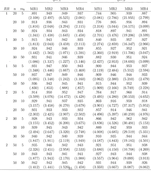
follow up 54 4.3 The estimated coverage probabilities and average lengths of confidence

inter-vals (in parenthesis) for the relative difference by the methods MR1, MR2,

MRS, MRA; for equal number of clusters rii = n0 = n in both groups, mean

cluster size m,o = 5,10, 50, RR = 1. 2; underlying mean probability of response

(17)

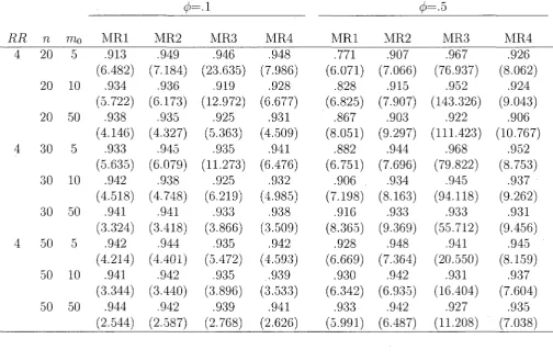
4.4 The estimated coverage probabilities and average lengths of confidence inter-vals (in parenthesis) for the relative difference by the methods MR.1, MR2,

MRS, MRA: for equal number of clusters tiy — n0 = n in both groups, mean

cluster size mo = 5,10, 50, R.R = 4; underlying mean probability of response

in group 0. TTO = 0.10 and a = 0.05; based on 10,000 simulations 56 4.5 The estimated coverage probabilities and average lengths of confidence

inter-vals (in parenthesis) for the relative difference by the methods RDR1, RDR2,

RDR3; for equal number of clusters n\ = no = n in both groups, mean

clus-ter size rriQ = 5,10,50, RED — 0.056,0.111; underlying mean probability of

response in group 0, TTO = 0.10 and a = 0.05; based on 10,000 simulations . . 57 4.6 The estimated coverage probabilities and average lengths of confidence

RDR3; for equal number of clusters ni = n0 = n in both groups, mean

clus-ter size mo = 5,10,50, RED = 0.167,0.222; underlying mean probability of

response in group 0, TTQ = 0.10 and a = 0.05; based on 10,000 simulations . . 58 4.7 The estimated coverage probabilities and average lengths of confidence

RDR3; for equal number of clusters n\ = UQ = n in both groups, mean

clus-ter size rriQ = 5,10,50, RED = 0.333,0.555; underlying mean probability of

response in group 0, ITQ = 0.10 and a = 0.05; based on 10,000 simulations . . 59

5.1 Frequency distribution of counts of embryonic death 81 5.2 Values of estimate of minus the log-likelihood (—/); estimates of // and c and

their standard errors in parenthesis; and estimate of the variance function with its standard error in parenthesis; for different values of b for embryonic

(18)

5.4 Values of estimate of minus the log-likelihood (—I); estimates of JJ, and c and their standard errors in parenthesis; and estimate of the variance function with its standard error in parenthesis; for different values b for redmites dataset 82 5.5 Variance function and the extended quasi-likelihood for the variance functions

(a) to (c) 82 5.6 Values of estimate of minus the extended quasi log-likelihood (—q), estimates

of j.i, c, cs and variance function (VF) along with their standard errors in

parenthesis for different variance functions for the embryo data set 82 5.7 Values of estimate of minus the extended quasi log-likelihood (—</), estimates

of (j,, c, OA and variance function (VF) along with their standard errors in

parenthesis for different variance functions for the red mite data set 82 5.8 Values of estimates of negative binomial log-likelihood (I), extended

quasi-likelihood for variance function v\ = /j, + cfj2 (qi), extended quasi-likelihood

for variance function v2 = c3n'2 (q2) and relative efficiency of estimates of \x

and V\, t>2 with respect to maximum likelihood estimates for all combinations of n = 20,30,50, /i = 2,5,10,20 and c = 0.1,0.2 for data generated from

gamma mixture of poisson 83 5.9 Values of estimates of negative binomial log-likelihood (I), extended

quasi-likelihood for variance function v\ = JJ, + C/J,2 (qi), extended quasi likelihood

for variance function t;2 = C3//2 (q2) and relative efficiency of estimates of /x

and V\, t'2 with respect to maximum likelihood estimates for all combinations of n = 20,30,50, /i = 2, 5,10,20 "and c = 0.4,0.6 for data generated from

(19)

5.10 Values of estimates of negative binomial log-likelihood (I), extended quasi-likelihood for variance function v\ = /i + c\i2 (q\), extended quasi likelihood

for variance function v2 = C3//2 (q2) and relative efficiency of estimates of /1

and v\, V2 with respect to maximum likelihood estimates for all combinations of n = 20,30,50, (i = 2,5,10,20 and c = 0.1,0.2 for data generated from log-normal mixture of poisson

5.11 Values of estimates of negative binomial log-likelihood (/), extended quasi-likelihood for variance function v\ = /1 + cfj2 (qi). extended quasi likelihood

for variance function v2 — c3/i'2 (g2) and relative efficiency of estimates of (j,

(20)

Chapter 1 X. n 1F o d u ciion

One often encounters clustered data in many applied sciences, such as epidemiology, preven-tive medicine, public health and toxicology. Clustered data refers to a set of measurements collected from subjects that are structured in clusters, where a group of related subjects constitutes a cluster, such as a group of students from the same class or rodents in the same litter. For instance, in toxicological studies there is a tendency among litter-mates to respond in the same way to stimuli, unlike animals from different litters. In this case, litters are clusters and the responses from litter-mates are correlated. Another example of clustered data is an intervention study where individuals in schools, clinics, classrooms, etc., are randomized into an intervention or control group. In such cluster-randomized designs, all patients of a clinician or all students from the same classroom or the same school are assigned the same treatment. These studies generate data that are clustered. Data analyses that do not appropriately account for the litter effects or the correlation among responses from individuals from the same classroom or the same clinic lead to erroneous statistical inferences.

(21)

instance, public health interventions, randomized control trials and environmental epidemio-logical studies which deal with developmental toxicology where one wants to study the effect of certain drugs, chemicals, and other environmental hazards that may put living beings at increased risk of various health problems. The second part deals with variance function selection in semi-parametric analysis of overdispersed count data.

In Chapter 2, we discuss some preliminaries and review the current literature.

In Chapter 3 we discuss interval estimation of the risk difference for clustered binary data. Risk difference (RD) is an important measure in epidemiological studies where the proba-bility of developing a disease for individuals in an exposed group, for example, is compared with that in a control group. There are varying cluster sizes in each group and the binary responses within each cluster cannot be assumed independent. Under the cluster sampling scenario, Lui (2004) discusses four methods for the construction of confidence intervals for the RD. In this chapter we introduce two new simple methods. One of these is based on an estimator of the variance of a ratio' estimator (Cochran, 1977) and the other is based on a sandwich estimator of the variance of the regression estimator using the generalized estimating equations approach of Zeger and Liang (1986). These two methods are then com-pared, by extensive simulations, in terms of maintaining nominal coverage probability, bias and average coverage length, with the four methods discussed by Lui (2004). Simulations show at least as good properties of these two methods as those of the others. The method based on an estimate of the variance of a ratio estimator performs best overall. It involves a very simple variance expression and can be implemented with a very few computer codes. Therefore it can be considered an easily implementable alternative.

(22)

construc-tion of confidence intervals for RED, namely, a method based on an estimate of the variance of a ratio estimator and Fieller's Theorem performs best overall. As in the case of the method recommended in Chapter 3 for the construction of a confidence interval for the risk difference, these methods also involve very simple variance expressions and can be considered as easily implementable alternatives.

In Chapter 5, we discuss some variance functions and make an attempt to determine an appropriate variance function (mean-variance relationship) which can be used in the semi-parametric analysis of count data. We use a hypothesis testing approach through a broader class of models and a data analytic approach. The models considered are the three parame-ter negative binomial distribution and the extended quasi-likelihood. We also derive a score test statistic and a likelihood ratio test statistic for testing if the parameter h in the three parameter negative binomial distribution is one, that is, to test if the negative binomial variance function is adequate. Our analysis shows evidence that the three parameter gener-alized negative binomial distribution NB{ji,c,b) does not improve in fit to count data over the simpler two parameter negative binomial NB(/j,,c) distribution. Moreover, the variance function of the NB(fj,,c.b) distribution does not have a closed form and is difficult to cal-culate numerically. So, for semi-parametric analysis we prefer the two parameter negative binomial variance function over the variance function of the three parameter negative bi-nomial distribution. Further data analysis and simulations using extended quasi-likelihood indicate that the negative binomial variance function and the variance function which ig-nores the linear term in the negative binomial variance function are preferable. The negative binomial variance function has almost full efficiency. The estimate of the variance function obtained by ignoring the linear term in the negative binomial variance function has efficiency below 1 only when the mean and the variance are small. Otherwise, in general, its efficiency is larger than 1.

(23)

Chapter 2 Literature Review

2.1 Inverse of patterned matrix

A patterned matrix that occurs quite frequently in probability and statistics, as well as other areas of interest and which occurred while deriving the sandwich estimator of variance of proportion for Chapter 3 and 4 in this dissertation, is the k x k matrix C defined by

C =

I a b

b a

b ... b a

(2.1)

This matrix can be written as

(24)

w here / is a k x k identity matrix and J is a k x k matrix of all unit elements given by

J

1 1

\

(2.2)

1 l

J

_kxk

Graybill (1983, Theorem 8.3.4, p. 190-191) has shown that

c-

1 _a~b_l_{a+(k- 1)6}

[I

jy

(2.3)

As indicated by Graybill, the inverse exists if and only if a ^ b and c ^ — (fc — 1)6. For a detailed proof see Graybill (1983, p.190-191).

2.2 Fieller

5

s t h e o r e m

Fieller's Theorem (Fieller, 1954) has been extensively reviewed by Casella and Berger (1990). In what follows, we describe Fiedler's theorem following Casella and Berger (1990).

Let (Xi,Yi), ..., (Xn,Yn) be a random sample from a bivariate normal population with

parameters (fj,x, I^Y, <J2X-, ^Y- P)- Further, let Z&i = Y{ — <5X,, for i = l , 2 , . , . , n , where

5 — IAY/^X- Then Z$ = Y — 5X and it can be shown that E(Z$) = 0 and Var(Zs) =

^(<7y + fi'2<Jx ~ ^Spayax)- Now, for convenience we denote Var(Z$) by Vs. Then, following

Hogg and Craig (1995, p. 214-217) it can be shown that Z$ ~ Ar(0,V^). An unbiased

estimate of Vs is Vs = n(n'_1) Yn=iizSi ~ ^}2, where zSt = y,, - Sxn and zs = y - 8x. Thus, Vs

can be written as

V

_{n(n - 1) fr{}1

_{X ^ ~y~}

s

(

Xi

-

x

)¥

(25)

where s

2y

= ^EILiI'^ - v?^

s

l = lELito -

x

?

a n d

«« = iYH=i{yi - v)(?i - x).*

Again, following Hogg and Craig (1995), it can be shown that V$ is independent of Z$ and

(n-l)Vs _ ^2 T>,,,c Jk

vs ~ Xln-iy T h u s' " 7 ^ ~ *(«-*) a n d

^ ( * < * ( n - l ) , « / 2 ) = l - « . ( 2 - 5 )

where £(n-i), a/2 is the 100(a/2)% point of the t-distribution with n — 1 degrees of freedom.

Then a 100(1 — a)% confidence interval for S can be found by solving zj = t'L^ a/2Vs or

equivalently by solving

t2 t2 t2

(x2 - _ Ln-1) 'a/2„ 2 ^x2 nf-~ L{n-l),a/2 ^ U | f_2 ''(n-l).a/2 ^

n

'^s2)52 - 2{xy - J^fsyx)5+ (;y2 - ^ f s 2 ) = 0, (2.6)

tj

which is a quadratic equation of the form ad2 — 2b5 + c = 0, where a = (x2 —("7)^)'1a/2-sz);

6 = (,xy - ^ f 7 2 ^ ) and c = (y2 - % z fz as2) - Then, for a > 0 and b2 - ac > 0,

solving equation (2.6) we obtain an approximate 100(1 — a)% confidence interval for 6 with boundaries

C f) * ( n - l ) , a/2Sy-i

x (n — l)x>2

9 T 7 « . .. 172 e2 i2_ ^ _,nsl/ .S2 ,<?2... \

(2.7)

*(n-.l), a/2 / S' I 2 7 / S ^ t/2 S2 ^ ( n - l ) , a / 2Sx / *2 ,S2:

a: y n — 1 x(n — 1) x2 n — 1 (n — l)x2 \n — 1 (n — l)s:j

where. C = , „n4"T2 2- Note that this interval is applicable for small n. For larger n (11 S.)X '(„_!), a/26a:

a further approximation can be used from the fact that as n —• 00, -f= ~ iV(0,1). Thus

2

P(^r<zll2) = l-a, (2.8)

where za/2 is the 100(a/2)% point of the normal distribution. Then, an approximate 100(1 —

(26)

we replace V$ by its estimate as n is assumed to be large. This leads us to the following

quadratic equation ,

A(Sy - 2B(S) + C = 0, (2.9)

where A = x2 — z^,2var(x), B = xy — -^jsyx and C = y2 - zl/2var(y). Then, the resulting

100(1 — a)% confidence interval for 8 is obtained solving

^ 4 ) 5 2 - 2(xy - ^sy*)8 + (f - | ^ ) = 0. (2.10)

n

Note that the interval obtained in this case is the same as that given in expression (2.7) with

t(n-i), a/2 replaced by za/2.

2.3 Cochran's m e t h o d for variance of a r a t i o e s t i m a t o r

Suppose yt and Xi are measured on each unit of a simple random sample of size n from a population of size N, and the population parameter to be estimated is the ratio R =

J2i=i 'Ihl Yl'i=i xi- An estimate of R is R = J21=i Vil YT%-=\ x%- ^n small samples the sampling

distribution of R is skewed and R is a biased estimate of R. Cochran (1977, Theorem 2.5, p.31) shows that as n —• oo, R is unbiased and V(R) = ^ 5 ^ - 1 • ^e furtner shows

that an estimate of V(R) is obtained by replacing i=1^i~i by = 1„i^ an(^ ^ ^y *'

For the detailed proof see Cochran (1977, p.31-33).

2.4 Quasi-likelihood

Quasi-likelihood was originally proposed by Wedderburn (1974) and discussed and applied by McCullagh and Nelder (1989), among others. Let yi, y2,..., yn be independent responses

(27)

regression parameters, fli, /32, • • •, PP, V(IJH) is a known function and (j> is a scale or a dispersion parameter. Then, the quasi-likelihood, or more appropriately, the quasi log-likelihood for a single observation y is given by

Q(M,=

.[w^

dt <2

-

n)

Since the components are independent by assumption, the quasi-likelihood (quasi log-likelihood) for the complete data is the sum of the individual contributions.

n

. Q O ; y ) =

^Qiiv-iWi)-2.5 Extended quasi-likelihood

The quasi-likelihood has a drawback in that it is not suitable for estimation of the overdisper-sion parameter. To overcome this, Nelder and Pregibon (1987) and Godambe and Thompson (1989) propose the extended quasi-likelihood by introducing a normalizing factor. Extended quasi-likelihood of the data can be written as

n

Q

+

(/xi,0,y) = X>2%{2^n</<)} + Q ( ^ ) ] ,

(28)

2.6 Generalized estimating equation and sandwich

es-. timator of variance

2.6.1 Marginal models

Let Yi = (Yn,... ,Yij,..., Yim.) , i = 1 , . . . , n and j = 1 , . . . , . . . , rrii be the response vector

and fii = (/iji,.... fMirii) be the corresponding mean vector. Further, let .Xy = ( a ^ i , . . . , XijP)

be the vector of explanatory variables for the jth measurement on ith subject and 0 =

(pi,... , 0P) be the corresponding p x 1 vector of regression parameters, which describes the

effect of explanatory variables on the marginal expectation of response. Then the marginal model as described in Liang (1999) consists of three components:

1. Systematic link g(jiij) = xijtd, where /Mj = E(Yij\xij).

2. Variance of Y^ given by Var(Ytj) = V(/%; <p), where <p is the overdispersion parameter.

3. Covariance specified as Cov(Yij,Yik) = C(fjLij,fj,ik] a), j < k = 1 , . . . .m,, where C is a known function such as Corr(Yij,Yiie) and a is the association parameter.

As given by Liang and Zeger (1986) and also discussed by Molenberghs and Verbeke (2006), the dispersion parameter can be estimated by cp = ^ YH=\ lt~ X^=i e% where e^ = y?~M'J .

Estimation of the association (or intraclass correlation) parameter a depends on the choice of the working correlation structure. For instance, if we assume exchangeable correlation, that is, Corr(Yij, Yik) = a, then a = \ YA=I mi(mt~-i) Sj#fc eye*fc- If we assume unstructured

correlation, that is, Corr(Yij,Yik)= a ^ , then a.jk = - Y^7=i eijeik- F°r further details see

Molenberghs and Verbeke (2006).

The regression parameter estimates are obtained by solving the following generalized estimating equations (GEE)

Sl(0,a) = J2^Cov~1(Yi]0,a){y^^(6)) = O (2.12)

(29)

for given a (see Liang and Zeger, 1986 for details). Since S\ depends on a, we iterate between solving Si(P,a(p)) = 0 for p and updating a(P) with the latest J3 obtained by solving equation (2.12) (Liang and Zeger, 1986).

2.6.2 Sandwich estimator of the covariaece matrix of j3

For estimating the covariance matrix of Q in marginal methods like generalized estimating equations, the sandwich estimator is often used. For further details see (Diggle, Heagerty, Liang and Zeger, 2002; Zeger and Liang, 1986). The sandwich estimator of Var(P) is given by

Vsandwich =Var0) =IQ1IJQ1

,-where

i= 1

and

h = ^ ( ^ ) ' ( 7 o t r1( F , ;/3 , a ) C o ^ ( ^ ) C 7 o t r1( Fi; , 5 , « ) ( ^ ) .

i = 1

Here Covt{Yi) is the true covariance matrix while Cov(Yi.p,a) is the working covariance

matrix given by Ai''Ri{a)Ai' /&, where A; = diag(V((j,i]),..., V()U„),..., V(j.iim.)) and

Ri(a) = Corr(Yij,Yik) is the working correlation matrix of Kj. Some common choices for

the working correlation assumptions (Molenberghs and Verbeke, 2006) in standard GEE are independence, that is, Corr(Yij,Yik) = 0 if j =£ k and 1 if j = k. exchangeability, that is,

Corr(Yij,Yik) = a and unstructured, that is, Corr(Ylj,Yik)= ajk- For computing Vsandwich,

(30)

2.7 Score test

Let I = 1(8, d),y) be the log-likelihood for the data y = (yi,...,yn) with parameters 9 =

(8i,...,9p) , where 6 is the parameter of interest and <f> = (0i,..,,0,s) is the nuisance

parameter. Suppose we wish to test HQ : 9 = 90 against H1 : 9 =£ 90. Further let ip =

dl I __ \dl 81 l | -. 81 I r 81 81 i\ r r-i/ d2l \ \ j ___

de\0=eo - [•mv->d6P\\o=9o> 7 - a$\o=e0 ~~~ [a$^ • • •' 848"e=e<» m ~ iH~aea07'lfl=fl°J> W

-£

("Wl«=«o)

a n d 7

«W» = ^ " W l ^ ' '

Now we define S = ^ — Bj^r, where B = htJ^ 1S ^i e partial regression coefficient matrix

obtained by regressing | | on ^-. The dispersion matrix of S is I0O4 = he — lo^I^J-^o-Then it can be shown (Neyman, 1959) that asymptotically, as n —» oo, S IQQ0S ~ \2p.

Next, if 0 in S and i^.^ is replaced by some \fn consistent estimator 0, then asymptotically, as n —> oo, S'I^QAS ~ Xp; where 5 and / ^ are obtained by replacing 0 by 0 in 5 and

Ige.cp- This is Neyman's C(a) test. Further, let 0 be the maximum likelihood estimate of

0 under H0, and -0 and I$gl ^ be the estimated values obtained by replacing 0 by 0 in -0

and I^Q^ respectively, then S is reduced to ip. The C(a) statistic then reduces to ip'I^^. Asymptotically, as n —• oo, ip'I^ip ~ Xp • This is the score test given by Rao (1947).

Thus, the score test is a special case of the C(a) test in which the nuisance parameters are replaced by maximum likelihood estimates. The score test is particularly appealing as it requires estimates of parameters only under the null hypothesis, and often produces simple forms of statistics, (Breslow, 1990; Paul and Banerjee, 1998).

2.8 Delta method

We use the delta method to derive an estimate of mean or variance of a transformation of one or more random variable(s). Suppose Tn = (Tni, T„2, . . . . TnN)' is asymptotically

(31)

has a non-zero differential <p = (<fii, <t>2, • • •, 4>N) at 0, where

dg

Then,

^[g(Tn) - g(0)] - ^ i V ( O , 0 ' S 0 ) . (2.13)

For large samples, g(Tn) has an approximate normal distribution with mean g(0) and

vari-ance </>'£<£/ri (see Agresti 1990, p. 422-423).

An illustration of the delta method given by Lui (2004) is as follows. Suppose the random vector {X\.X2)... ,Xn) follows the multinomial distribution with parameters n

and 7r = (7Ti,7r2,... ,7rn)'. By the central limit theorem, if n is large the random vector

•fr = (7T!, 7T2,..., 7rn) asymptotically has the multivariate normal distribution with mean

TV = (TT\,TT2,. • •,7rn)' and covariance matrix S* = \diag{iv) — 7cn ]/n, where TTJ = Xjjn,

and diag(n) is a diagonal matrix with diagonal elements equal to 7Tj. Suppose the function

gi^i-, ?2; • • • - TTJV) n a s a non-zero differential TT* = (7r*, 7r2, .. •, K*N) at TT, where

(32)

Chapter 3 Interval Estimation of Risk Difference

for Clustered Binary D a t a

3.1 Introduction.

Cluster sampling is often employed in epidemiological cohort studies to compare the proba-bility of binary responses in an exposed group with that in a control group.

Consider the example given in Lui (2004, p.7) of a study of an educational intervention program on behavior change with regard to solar protection (Mayer, Slymen, Eckhardt 1997). The data consisted of 29 classes in each of the intervention and the control group with class sizes ranging from 1 to 6 in the intervention group and from 1 to 4 in the control group. For a similar set of data, see Lui (2004, p.7) and Cochran (1977, p.67).

The data, reproduced in Table 3.1, consist of 29 clusters (classes) of varying sizes (number of children in each class) in each of the intervention and the control group. Let TTI be the probability that an individual (a child) in the intervention group does not have adequate level of solar protection and 7r0 be the corresponding probability in the control group. Often,

it is of interest to estimate the risk difference RD = A = TTI —

(33)

each cluster are independent. Such an analysis would bias the inference procedures regarding A as observations within a cluster are likely correlated. Newcombe (1998) evaluates eleven methods for constructing a confidence interval for A for non-clustered data. Of these eleven methods he proposes a new method (method 10 in his paper). Newcombe remarks that the new method and a continuity corrected version of it (method 11 in his paper) are remarkably simple and have good properties. For clustered data, Lui (2004) reviews four methods of which one method is an extension of Newcombe's method 10.

In this chapter we introduce two very simple methods. One of these is based on an estimator of the variance of a ratio estimator (Cochran 1977, p.31) and the other is based on a sandwich estimator of the variance of the regression estimator using the generalized estimating equations (GEE) approach of Zeger and Liang (1986). We then compare these two methods, by simulation, in terms of maintaining nominal coverage probability and av-erage covav-erage length, with the four methods discussed by Lui (2004). In section 3.2 we briefly review the four methods discussed in Lui (2004) and introduce two new methods. A simulation study is conducted in Section 3.3. Three examples are given in Section 3.4 and a discussion follows in Section 3.5.

3.2 Review of some existing p r o c e d u r e s by Lui (2004)

(34)

risk factor. We assume further that the binomial probability Pij is a random variable having mean 7r* and variance 7Tj(l — TTi)fa. The unconditional mean and variance of .-%, then, is

rtiijiii and m,ijTXi(l — 7Tj)(l + (m^- — I) fa) respectively. Note that the parameter fa is the

common intraclass correlation between the binary observations within each cluster in the ith group.

Method LI:

The unbiased estimate of 7r,; is 7r,; = Xi./rrii., where Xi. = Y^jL\xiji m*. = E j i i m*i a nd

therefore, an unbiased estimate of A is TTI — TT0. Using Lindeberg's central limit theorem, the

estimator A has, asymptotically, a normal distribution with mean A and variance Var(A) —

Yli=Q7ri(l ~ 7rj.)/(mij (/}i)/rni-i where m; = (run,rrii2, • • •, m m j and the variance inflation

factor due to intraclass correlation coefficient is given by f^mi^fa) = ErrK?'[l + (mu ~

l)fa]/rrii.. The proof of this result is given in Appendix A.l. An asymptotic 100(1 — a)%

confidence interval for A then is

[max [A — ZQ/2"Jvar(A), — 1], rain [A + Za/2y var(A), 1]],

where var(A) is obtained by replacing TT, and fa, i = 0,1, in war (A) by their estimates 7?* = Xijrrii. and fa = {BMS, - WMS^/lBMS, + (m* - 1)WM5J, where BMSi =

E i ^ S / ^ - C E i ^ O V E i ^ - l / C n i - i ) ^ d wMSi =

[E;*;-E;(*§Mi)]/(E;(™y-1)) are 'between mean squared' errors and 'within mean squared errors' respectively and

mt — [ ( E jmi j )2 ~~ E imf j ] / [ (ni ~~ l ) E jmy ' l - The above analysis of variance (ANOVA)

type estimate of the intraclass correlation fa was first proposed by Elston (1977) for cor-related continuous data and later used by others, such as Donner et al. (1981) and Lui et al. (1996). The derivation of the above analysis of variance (ANOVA) type estimate of the intraclass correlation fa is given in Appendix A.2.

Method L2:

(35)

nii. (it is usual in practice to have small m7;/s as in the datasets in Table 3.1 and Table-3.2),

which can produce an inaccurate confidence interval for A. A better method would be to construct the confidence interval using the fact that A has, asymptotically, as m*. becomes large, a normal distribution with mean A and variance Var(A). Then, an approximate confidence interval for A can be constructed using the fact that for large mi.,

F(((A - A ) /v/ y a r ( A ) )2 < Z*/2) = 1 - a. (3.1)

Now, let r = 7Ti + 7T0, A+ = 1 + c ( m » Z £/ 2/ 4 , B+ = A + (1 ^ [ / ( m i ^ / m i .

-m0,d)0)/m0]Zl/2/4, C+ = A + r(2- r)c(m, <j>)Z2a/Jl, where, c(m, <p) = £ j= 0 /(™i> &)M->

m'x = (mn,mi2, • • • , m-m,) and m^ = (moi,m02, • • • , Won0)- Then, by solving the quadratic

equation in (3.1) and replacing r by ft = TTI + TVQ and (pi by its ANOVA estimate in A+, B+

and C+, an asymptotic confidence interval for A is obtained as

[A/(fi),Au(fi)],

where At(r\) = max {(B+ - V#+2 - A+C+)/A+,-l} and

Au(fi) = m m { ( B+ + \/B+2 — A+C+)/A+, 1} are the two distinct roots in the interval

(-1,1) such that the equality in (3.1) holds. Now, define IT* — (xi. + 0.5)/(mi. + 1). When either of TT0 and TT-J is 0 or 1, we use r* = TTJ + TTQ to estimate r.

Method L3:

Following Beal (1987) we use r* defined in Method L2 irrespective of whether or not TTJ is 0 or 1.

Method L4:

Nqte that, asymptotically, as rii —> oo, 7tj ~ N^i,ir^l — 7Tj)/(mi,0j)/mi.). Then, an asymptotic 100(1 — a)% confidence interval for in can be obtained as a solution of

(36)

i = 0,1. Let li and Ui be the smaller and larger roots of the quadratic equation of TTJ obtained

from (3,2). Then, following Newcombe (1998). an asymptotic 100(1 — a)% confidence interval for A is

[max{A - Za/2\Jli{l - U)f{m.1,(j)y)/ml. + u0(l - u0) / ( m0, (po)/rn0., - 1 } ,

min{k + Za/2\Jui(l - Ui)f(m1,<j)i)/mi. + k(l - /0) / ( m0, 4>o)/m,Q.., 1}]. (3.3)

3.3 Proposed methods for estimate of variance of A

3.3.1 The method based on the estimate of variance of a ratio

estimator

As we have discussed earlier, the estimate of TTJ is ifi = Xi./rrii. where x%_ = Y^j=\xij a nd

rrii. = Y^j=imiy This can be written as the ratio of two sample means, £i = Xi/m,i, where

%i = Xijrii and fhi = rriijni. Then, using a result from Cochran (1977) of the estimate of

the variance of a ratio estimator, an estimator of the variance of m is

""» ,v.2

_____ ' ni s^ {Xij — 7T,:mij) _ n% ^ ^ ri

Vi —

ru

_ V ^ VLiJ ~ »i"Hj) _____ 'H y ^ lij_ ,g ^

j = l l- 3=1

where r„ = x*y — 7fjm.y. Following Scott and Wu (1981), one can show that (TTJ — it^/v'* is asymptotically iV(0,1) as n* —> oo under the following mild regularity conditions on the population variances of t h e m e ' s and r^s:

• Total sum of squares of the r^'s from gross outliers about the line joining (rhi, x~i) to

the origin should be relatively small.

(37)

Further, vt is a consistent estimator of var(yfj) in the sense that rti\vi — var(-Ki)] converges in

probability to 0 as n, —* oo, for each i. For proof see Appendix A.3, The ratio of vi to the estimated binomial variance represents the variance inflation due to clustering and is also known as design effect in survey sampling literature (Kish, 1965). Using these properties of iti, Rao and Scott (1992) developed a test for comparing several independent groups of clustered binary data with group specific covariates.

It can then be seen that, asymptotically, as ru —>• oo, (ifi — if0) ~ N(TTI — 7ro,t>i + i>o), so that,, as B0 —• oo and n\ —> oo,

(7f1-7ro)-(7r1-Tro) ^ ^ ( Q , 1 ) .

Method CI:

Thus, an approximate 100(1 — a) confidence interval for the risk difference A = TTJ — TTQ is obtained as (TT\ — TTQ) ± Za/2 \ / ( f o + V\). Note that this method does not assume any specific

model for overdispersion or intraclass correlation. As in Method L2 we replace 7fj by ir* in

i>i if iTi is 0 or 1 , where n* = (XJ.. + 0.5)/(TOJ. + 1). Method C2:

As in Method L3 we replace TTJ by TT* in Vi irrespective of whether or not vfj is 0 or 1.

3.3.2 The method based on t h e sandwich estimator of t h e

vari-ance of the regression estimator

Zeger and Liang (1986) propose an estimating equations approach for estimating regression parameters for longitudinal data. They also provide a robust estimator, called the sandwich estimator, of the variance of the regression estimator. In Appendix A.4, we theoretically apply their method to the basic binary data, which are not available to us, to obtain an estimate of a proportion from clustered correlated binary data and an estimate of its variance. Using these results we obtain an estimate of nt, i=0, 1,

(38)

and an estimator of the variance of TTJ

n.i

Note that the estimate of TTJ is the same as that obtained earlier and, as in Vi, the sandwich estimator vSi does not require knowledge of the basic binary data. Corresponding to the

methods Cl and C2, two more confidence intervals, denoted by SI and S2, are obtained by replacing v.j, by vSi. Further, note that Vi = (rii/(Bj — l))vSi. Therefore, a confidence interval

for A based on Vi will have larger coverage probability and coverage length.

3.4 Simulation studies

In this section we report on a simulation study conducted to compare the eight methods LI, L2, L3, L4, C l , C2, SI and 52 in terms of coverage probabilities and-average coverage lengths. For simplicity we consider equal numbers of clusters UQ = n\ = 29 (same as those in the data in Table 3.1). Four cluster size configurations, (a) all cluster sizes equal to 2, (b) all cluster sizes equal to 4, (c) all cluster sizes equal to 40, and (d) cluster sizes the same as those in the data in Table 3.1, are considered. A common value of TT0 = .20 and eight values

of A = 7ri - 7T0= 0.0, 0.05, 0.1, 0.2, 0.3, 0.4, 0.5, 0.7 are considered. We consider equal

values of the over-dispersion parameters (p = 0.05, <p — 0.10 and <b = 0.32 in the control and treated groups and unequal values of 60 = 0.324 in the control group, and <p\ = 0.249 in the

treatment group (these values were taken as the maximum likelihood estimates of tpo and <p\, based on a beta-binomial model, for the data in Table 3.1). Data in the control group were generated from a beta-binomial distribution with mean TTO and over-dispersion parameter c6 and those in the treatment group were generated from a beta-binomial distribution with mean TT\ and over-dispersion parameter <b.

(39)

did not exist for some samples. These samples were rejected. Note that if both BMSi and

WMSi are 0 then the estimate of (pi, used in the methods LI, L2, L3 and L4, is not valid.

Further, confidence intervals by the methods L2 and L3 do not exist if B+2 — A+C+ < 0.

where A+ = 1 + c(m,<t>)^/2/4, B+ = A + (1 - r ) [ / ( m i , ^ ) / m i . - / ( m0, <Po)M>.]^/2/4>

C+ = A + r(2 — r)c(m, 0)Z^/2/4 and c(ra, 0) = J2i=o f(mu <Pi)/mi. • Thus coverage

proba-bility and average length were based on 10,000 samples in which a confidence interval existed for all methods (good samples). The coverage probability for A obtained, is then equal to the number of times the confidence intervals contained the true value of A/10,000. For each of the 10,000 good samples, the length of the confidence interval was calculated. The average coverage length (average length) is the mean of these 10,000 lengths. The number of samples rejected, in general, was small (in 10,000 samples, 0 to 80 samples were rejected). However, for some large values of (p, this number was substantial (ranging from 200 to 4010).

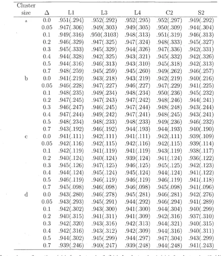
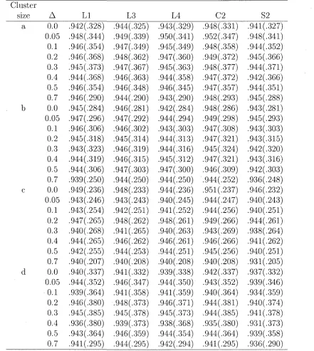
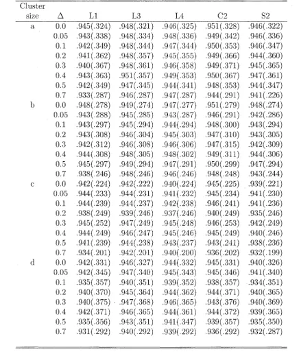
The empirical coverage probabilities, the average lengths and bias properties are almost identical for Methods L2 and L3, although method L3 provides slightly better coverage probabilities in some situations. Similarly, the method C2 is slightly better than the method CI. The methods Si and S2 show almost identical empirical coverage probabilities and average coverage lengths. So, to save space, we present simulation results for only five methods LI, L3, L4, C2 and 52. The empirical coverage probabilities and average lengths for common values of the over-dispersion parameters (p = 0.05, cp = 0.10, and <p = 0.32 are given in Table 3.3, Table 3.4, and Table 3.5 respectively. The corresponding biases of the confidence intervals (coverage probability -.95) are plotted in Figure 3.1, Figure 3.2 and Figure 3.3.

(40)

probability. '

Simulation results in these tables indicate that all methods maintain nominal coverage reasonably well, although method C2 has some edge in terms of correct coverage probabil-ities (that is, it attains correct coverage probability 0.95 in more situations than any other method). Note that the bias of the confidence interval by the new method C2, in general, is the smallest (see Figure 3.1 to Figure 3.3) and that by the GEE method S2, in general, is the largest. In terms of average length, nearly similar performance is shown for all procedures. The average coverage length decreases as the cluster size increases (see the results for cluster size configurations a, b, and c). For unequal cluster size situation (see the results for cluster size configuration d) the empirical coverage lengths for all methods are of similar magnitude for smaller values of <p (0.05 and 0.10). For larger value'of 0 (0.32), the method C2 seems to give somewhat larger lengths.

(41)

remain the same as those found earlier (in Tables 3.3-3.5) for the mesial end. For the distal end, in general, the coverage is smaller than the nominal 95% coverage level for all methods. However, for the LI, C2 and 52 methods, it is never below 0.85. For the other two methods, L3 and L4, coverage becomes very small and even goes to zero in some cases in which cluster-sizes are small. For example, for cluster size configuration (a), empirical coverage was found to be zero for all values of A used in the simulation. However, this situation improves as the cluster sizes increase. For example, for cluster size configuration (c) in which all cluster sizes are 40, empirical coverage ranged from 0.762 to 0.951.

3.5 Examples

E x a m p l e 1. In this example we consider the data discussed in Section 3.1 and given in Table 3.1. We are interested in finding a confidence interval for the difference in prevalence rates A = n\ — TTO of children who do not have adequate level of solar protection.

For these data, we obtain ifj = 0.422, TTQ = 0.618 and the estimate of the common

intra-class correlation <j> = 0.30. The 95% two sided confidence intervals for A by the five methods LI, L3, L4, C2 and 52 are (-0.405,0.013), (-0.392,0.017), (-0.385,0.016), (-0.412,0.026) and (—.409, .022) respectively. The corresponding lengths of the confidence intervals are .418, .409, .401, .438. and .430.

E x a m p l e 2. We now consider data from treatment 1 representing some low dose of a compound from a teratological experiment (Paul, 1982) and data from the control group. The data are given in Table 3.2. The data refer to litters of varying sizes, each litter having a number of abnormalities. For more details about the data, see Paul (1982). Now, let 7Ti be the proportion of abnormalities in the treatment group and TTQ be the proportion of abnormalities in the control group. We are interested in estimating the difference A = -K\— TTQ.

(42)

(-0.107,0.105), (-0.110,0.108), (-0.108,0.105) and (-.105,0.102) respectively with cover-age lengths 0.213, 0.212, 0.218, 0.213 and .208.

The score test statistics (Tarone, 1979; Paul, 1982) with p-values in parenthesis for testing for over-dispersion in the treatment group and the control group in example 1, are 3.017 (0.001) and 2.509 (0.006) respectively. The corresponding values for the two groups in example 2 are 2.568 (0.005) and 4.697 (< 0.001) . All data sets show evidence of over-dispersion. Thus, all the methods discussed here for confidence intervals that take into account over-dispersion, are appropriate.

In example 1, the confidence intervals for methods LI, L3 and LA are similar and their lengths are also similar. The confidence interval and the length for method C2 is somewhat different from those of LI, L3 and L4. The length of intervals for methods C2 and S2 are larger than those of methods LI, L3 and L4. In example 2, the confidence intervals for all methods are similar and the lengths for all methods are also similar.

E x a m p l e 3. As identified by Newcombe (1998), there are four boundary cases, NZ (no zero cells), OZ (one zero), RZ (two zeros in the same row) and DZ (two zeros on the same diagonal). Cases RZ and DZ imply that no clustering was observed. Example 1 and example 2 both illustrate the NZ case. In this example we try all methods on an OZ case. The data are 5/10, 4/10, 1/10, 0/10 vs 0/10, 0/10, 0/10, 0/10. For these data, however, the values of BMS0 and WMSQ are 0. Thus the value of the estimate of cp0, used in the methods LI,

L2, L3 and L4, is not valid and therefore the confidence intervals by LI, L2, L3, L4 methods do not exist. The confidence intervals for the C2 and S2 methods exist, and are (.016, .484) and (.047, .452) with corresponding lengths .468 and .405 .

3.6 Results and discussion

(43)

(Cochran, 1977) and the other is based on a sandwich estimator of the variance of the regression estimator using the generalized estimating equations approach of Zeger and Liang (1986). These procedures stand out with respect to computational simplicity. One of the existing procedures, namely, L4, shows larger average coverage lengths in some situations, otherwise all procedures have similar average coverage lengths. Method C2 computed the confidence interval as

(ifi - 7f0) ± ZQ/2y/(vo + Vi), (3.5)

where v{ = (^/(n,- - l ) ) X ) " l i (xy ~ mij^i)2/mt- a n d ** - (Xi. + 0.5)/(mj. + 1), and is

preferable as it is always computable and its overall performance is better than the other procedures. For example, method C2 attains correct coverage probability 0.95 in more situations than any other. This method, in general, also has the best bias and symmetry properties. A further advantage of this method is that the confidence interval, as evidenced from simulations, always remains within [-1, 1].

(44)

Table 3.1: Radiation exposure data. (Mayer et al., 1997). (i) Class sizes, (ii) Observed number of children with an inadequate level of solar protection.

Groups

Intervention (i) 3 2 2 5 I 3 1 2 2 2 I 3 I 3 2 2 6 2 4 2 2 2 2 1 I 1 I 1 T

(ii) 1 1 1 0 1 2 1 2 2 1 1 2 1 2 2 0 0 0 0 1 2 1 1 1 1 0 0 0 0

Control (i) 2 4 3 2 3 4 4 2 2 3 2 2 4 3 2 3 1 1 2 2 2 3 3 4 1 1 1 1 1

(ii) 0 0 2 2 0 4 2 1 1 3 2 1 1 3 2 3 1 0 1 2 1 1 2 4 1 1 1 0 0

Table 3.2: Toxicologic^! data. (Paul, 1982). (i) Number of live fetuses affected by treatment, (ii) Total number of live fetuses.

Groups

Dose.L (i) 5 11 7 9 12 8 6 7 6 4. 6 9 6 7 5 9^ 1 6 9^

(ii) 0 1 1 0 2 0 1 0 1 0 0 3 0 0 1 5 0 0 3

ControLC (i) 12 7 6 6 7 8 10 7 8 6 11 7 8 9 2 7 9 7 11 10 4 8 10 12 8 7 8

(45)

Table 3.3: Coverage probabilities, average lengths of confidence intervals for the risk differ-ence A by the methods LI. L3, LA, CO,, 52; equal number of clusters n\ = no = 29 in both groups; 7T0 = 0.20. <p = 0.05; a = 0.05; based on 10,000 simulations

Cluster A 0.0 0.05 0.1 0.2 0.3 0.4 0.5 0.7 0.0 0.05 0.1 0.2 0.3 0.4 0.5 0.7 0.0 0.05 0.1 0.2 0.3 0.4 0.5 0.7 0.0 0.05 0.1 0.2 0.3 0.4 0.5 0.7 LI .951( .947( .949( .946( .945 ( .944( .944( .948( .941( .9461 .948( .947( .946 ( ,947( .948( .943( .941( .942( .942 ( .940 ( .945 ( .9441 .946 .945( .943( .943( ..942( .940 ( .942 .942 .944 .939 ,-294) .306) '.316) . .329) .333) .328) v.316) '.259) .219) .228) ,.235) ^.245) .247) .244) .234) '.192) ,.111) .116) ;.ii9) '.124) ;.i26) '.124) .119) .098) .280) .293) ,.302) \315) ;.320) ,.316) ,.302) '.246) L3 952 949 950 ( 947( 945 ( 942 ( 946! 945( 943( 947( 949 947 946 949 ( 948( 946 ( 942( 942( 941( 940( 947 945 946 946 ( 946( 945( 943( 941 ( 943 943 945 940 ,.292; .303; 3103 .325; ;.329; ;.325; ;.3i3; '.259; .218; ,.227; i-234; ;.243; .245; .242; ;.233; ;.i92; '.111; ; . i i 5 ; '.119; '.124; '.125^ '.124^ .119^ .098; .278; .291; ,.300; .311; ,.3i6; ;.3i2; ^.299; .247^ L4 .952 .949 ) .948 .947 .944 .943 .943 .945 .943 .946 .948 .947 .947 .947 .948 .944 .941 .942 .941 .939 .946 .945 .946 .946 .945 .944 .941 .941 .942 .942 .944 .939 ;.295) '.305) '.313) ,.324) ,.326) !-321) ;.3io) ;.260) ;.2i9) j.227) ;.234)

J.242)

.244) ,.241) ;.233) '.193) Mil) M16) M19) M24) M25)

1-124)

".119) '.098) ;.281) ;.292) ;.3oo) M09) ;.3i3) ;.309) ;.297) '.248 C2 .952 .950 .951 ( .948( .947( .945( .945( .949( ,942( .947! .950 .948 .948 .948! .949! .944! .942( .942( .943! .941! .945 .944 .946 .945! .946( .946! .944! .942! .944 .944 .947 .944 '.297) .309) .319) .333) .336) .332) ,.318) '.262) .219) '.229) ;.236) ;.246) .248) .245) .236) .193) .111) .115) M19) ,.124) M25) ,.124) .119) .098) .281) .294) ,.304) ;.316) ;.321) ;.3i6) '•304) '.248) S2 949! 944 946 ( 945 ( 942( 942( 942( 946( 940( 941( 945 944 943 943( 946! 940( 939( 939( 938( 936 942 941 941 941( 942( 941( 940! 937 940 940 943 941 ;.292 .304 .313 .327 .331 ,.326 ,.313 |.257 '.216 ;.225 ;.232 ;.24i .244 .241 .232 .190 '.109 '.114 M17 M22 M23 M22 ,.118 '.096 .276 '.289 ;.299 ;.3io ;.3i5 ;.3ii ;.299 '.243

(46)

Table 3.4: Coverage probabilities, average lengths of confidence intervals, ence A by the methods LI, L3, LA, C2, S2; equal number of clusters n-{ groups: 7To = 0.20, cp = 0.10; a = 0.05: based on 10,000 simulations

Cluster

size A LI L3 L4 C2

a 0.0

0.05 0.1 •0.2 0.3 0.4 0.5 0.7 0.0 0.05 0.1 0.2 0.3 0.4 0.5 0.7 0.0 0.05 0.1 0.2 0.3 0.4 0.5 0.7 0.0 0.05 0.1 0.2 0.3 0.4 0.5 0.7 .948 .946 .952 .947 .947 .947 .944 .948 .948 .941 .945 .947 .947 .942 .944 .939 .941 .945 .944 .946 .943 .942 .942 .943 .944 .947 .944 .943 .939 .944 .941 .938

for the risk differ-= no differ-= 29 in both

S2 (.301) (.314) (.324) (.337) (.341) (.337) (.324) (.265) (.232) (.242) (.249) (.259) (.263) (.260) (.250) (.204) (.143) (.149) (.154) (.160) (.162) (.160) (.154) (.126) (.292) (.305) (.315) (.328) (.333) (.328) (.315) • (.256) 949(.298) 947(.311) 952(.320) 949(.333) 946(.336) 948(.333) 945(.320) 945(.266) 948(.231) 942 (.240) 946 (.248) 949 (.257) 947(.261) 941(.257) 944(.248) 943(.204) 940(.143) 945(.148) 943(.153) 947(159) 943(.161) 942(.160) 943 (.153) 945(.126) 946(.290) 947(.302) 945(.311) 943 (.324) 940(.329) 944(.323) 941(.312) 938(.256) 949(.301) 946(.312) 951(.321) 948(.331) 946(.333) 946(.329) 943(.316) 947(.266) 947(.233) 942 (.241) 945(.248) 948(.256) 947(.259) 940(.256) 941(.246) 943(.205) 939(.143) 944(.149) 942(.153) 947(.159) 943(.161) 943(.159) 943(.153) 944(.126) 946(.293) 946(.303) 942(.311) 943 (.322) 940 (.326) 944(.320) 942(.309) 935(.257) 951 (.303) 948(.316) 954(.327) 949 (.340) 948(.344) 950 (.340) 946(.327) 948(.268) 949(.233) 944(.243) 947(.251) 949(.261) 949(.264) 944(.261) 945(.251) 940(.205) 942(.143) • 946(.149) 944(.154) 947 (.160) 944 (.162) 942(.161) 943(.154) 944(.126) 945 (.293) .948(306) 947(.316) 947(.329) 940 (.334) 943 (.329) 943(.316) 942(.257) 946(.298) 943(.311) 950(.321) 945 (.335) 943 (.338) 946(.335) 943(.321) 945(.264) 946(.229) 939 (.239) 943(.247) 945(.256) 943(.260) 939 (.257) 941 (.247) 936(.202) 937(.141) 942(.146) 939(.151) 943(.158) 939(.159) 938(.158) 938(.151) 939(.124) 941(.288) 944(.300) 942(.310) 941(.323) 936(.329) 938 (.323) 938(.311) 937(.253)

(47)

Table 3.5: Coverage probabilities, average lengths of confidence intervals, ence A by the methods LI, L3, L4, C2, ,5*2; equal number of clusters n\ groups; 7T0 = 0.20, <p = 0.32; a = 0.05; based on 10,000 simulations

Cluster

size A a

b

LI L3 L4 C2

0.0 0.05 0.1 0.2 0.3 0.4 0.5 0.7 0.0 0.05 0.1 0.2 0.3 0.4 0.5 0.7 0.0 0.05 0.1 0.2 0.3 0.4 0.5 0.7 0.0 0.05 0.1 0.2 0.3 0.4 0.5 0.7

for the risk differ-= UQ differ-= 29 in both

S2 .942(.328) .948(.344) 946 (.354) 946 (.368) 945 (.373) 944(.368) 946(.354) 946(.290) 945(:284) 947(.296) 946(.306) 945(.318) 943(.323) 944(.319) 944(.306) 939(.250) 949(.236) 943 (.246) 943 (.254) 947(.265) 940(.268) 944(.265) .942(.255) .940(.207) .940(.337) .944(.352) .939(.364) .946(.380) ,945(.385) .936(.380) .943(.364) .941 (.295) 944(.325) 949(.339) 947(.349) 948(.362) 947(.367) 946(.363) 946(.348) 944(.290) 946(.281) 947(.292) 946(.302) 945(.314) 946(.319) 946(.315) 947.(.303) 944(.250) 948(.233) 943(.243) 942(.251) 948(.262) 941 (.265) 946(.262) 944(.253) 940(.208) 941(.332) 946 (.347) 941(.358) 948(.373) 945(.378) 939(.373) 946(.359) 944(.295) 943(.329 950(.341 945(.349 947(.360; 945(.363; 944(.358; 946(.345; 943(.290; 942(.284; 944(.294; 943(.303; 944(.313; 944(.316; 945(.312] 947(.300; 944(.250; 944(.236; 940 (.245; 941(.252; 948(.26l' 940C.263, 946(.261^ 944(.25l' 940(.208; 9390338, 944(.350' 941(.359y 946(.37l' 945 (.373 938(.368 944(.354 942(.294 ) .948(.331) ) .952(.347) .948(.358) ,949(.372) .948(.377) .947(.372) .947(.357) .948(.293) .948(.286) .949(.298) ,947(.308) .947(.321) .945(.324) .947(.321) .946(.309) ,944(.252) .951 (.237) .944(.247) .944(.256) .949(.266) .943(.269) .946(.266) .945(.256) .940(.208) .942(.337) .943(.352) .940(.364) .944(.381) ,944(.385) } .935(.380) ) .944(.364)

} .941 (.295)

941 (.327) 948(.341) 944(.352) 945 (.366) 944(.371) 942(.366) 944(.351) 945(.288) 943(.281) 945(.293) 943 (.303) 943(.315) 942(.320) 943(.316) 942(.303) 936(.248) 946(.232) 940(.243) 940(.251) 944(.261) 938 (.264) 941 (.262) 940(.251) 931 (.205) 937(.332) 939 (.346) 934(.359) 940(.374) 941 (.378) 931 (.373) 939 (.358) 936 (.290)

(48)

(49)

Table 3.7: Coverage probabilities and average lengths of confidence intervals, for the risk difference A by the methods LI, L3, L4, C2, 52; equal number of clusters rt\ = no = 29 in both groups; TTQ = 0.20, <f>o = 0.324, (pi = 0.249; a = 0.05; based on 10,000 simulations

Cluster size

a

A LI L3 L4 C2

0.0 0.05 0.1 0.2 0.3 0.4 0.5 0.7 0.0 0.05 0.1 0.2 0.3 0.4 0.5 0.7 0.0 0.05 0.1 0.2 0.3 0.4 0.5 0.7 0.0 0.05 0.1 0.2 0.3 0.4 0.5 0.7 S2 .945(.324) .943(.338) .942(.349) .941(.362) .940(.367) .943(.363) .942(.349) .933(.287) .948(.278) .943(.288) 943(.297) .943(.308) .942(.312) .944(.308) .945(.297) .938(.246) 942 (.224) .944(.233) .944(.239) .938(.249) .945(.252) .944(.249) 941(.239) .934(.201) .942(.331) .942(.345) .935(.357) .940 (.370) .940(.375) • .942(.371) .935(.356) .931(.292) 948(.321 948(.334 948(.344 948(.357 948(.361 951(.357 947(.345 946(.287 949(.274 945(.285 945(.294 946(.304 946(.308 948(.305 949(.294 948(.246 942(.222 944(.231/ 944(.237 939(.246^ 947(.249 946(.247 944(.238 942(.20r 946(.327 947(.340 940 (.351 945 (.364 947(.368 946(.365: 943(.351 940(.292 ) .946(.325) ) .948(.336) ) .947(.344) ) .945(.355) ) .946(.358) ) .949(.353) ) .944(.341) ) .947(.287) ) .947(.277) ) .943(.287) ) .944(.294) ) .945(.303) ) .946(.306) ) .948(.302) ) .947(.291) ) .946(.246) ) .940(.224) ) .941 (.232)

) .942(.238)

) ,937(.246) ) .945(.248)

) .945(.246)

) .943 (.237) ) .940(.200) ) .944(.332) ) ,945(.343) ) .939(.352) ) .944(.362) ) .946(.365) ) .944(.361) ) .941(.347) ) .939(.292) 951 (.328) 949(.342) 950(.353) 949(.366) 949(.371) 950(.367) 948 (.353) 944(.291) 951(.279) 946(.291) 948(.300) 947(.310) 947(.315) 949(.311) 950 (.299) 948(.248) 945(.225) 945(.234) 946(.241) 940(.249) 946 (.253) 945(.249) 943(.241) 936(.202) 945(.331) 945 (.346) 938(.357) 944(.371) 943(.376) 944(.372) 939(.357) 936(.292) 946(.322) 946(.336) 946 (.347) 944(.360) 945(.365) 947(.361) 944(.347) 941(.226) 948(.274) 942 (.286) 943(.294) 943 (.305) 942(.309) 944 (.306) 947(.294) 943 (.244) 939(.221) 941 (.230) 941 (.236) 935(.246) 942 (.249) 940 (.246) 938 (.236) 932(.199) 940(.326) 941 (.340) 934(.351) 940 (.365) 940 (.369) 939(.365) 935(.350) 932(.287)

Inference on some epidemiological indices and variance function in semi-parametric analysis of count data

Scholarship at UWindsor

Scholarship at UWindsor

Inference on some epidemiological indices and variance function

Inference on some epidemiological indices and variance function

in semi-parametric analysis of count data

in semi-parametric analysis of count data

I N F E R E N C E ON SOME E P I D E M I O L O G I C A L INDICES

AND V A R I A N C E F U N C T I O N

IN SEMI-PARAMETRIC ANALYSIS O F COUNT DATA

by

Tasneem Zaihra

A Dissertation

Submitted to the Faculty of Graduate Studies

through the Department of Mathematics and Statistics

in Partial Fulfillment of the Requirements for

the Degree of Doctor of Philosophy at the

University of Windsor

Windsor, Ontario, Canada

2009

1*1

Declaration of Previous Publication

Abstract

Dedication

A c k n o w l e d g e m e n t s

Contents

ist of Figures

ist of Tables

Chapter 1

X. n 1F o d u ciion

Chapter 2

Literature Review

2.1 Inverse of patterned matrix

J

c-

[I

jy

2.2 Fieller

s t h e o r e m

V

X ^ ~y~

(

-

)¥

where s

= ^EILiI'^ - v?^

l = lELito -

?

««* = iYH=i{yi - v)(?i - x).

2.3 Cochran's m e t h o d for variance of a r a t i o e s t i m a t o r

2.4 Quasi-likelihood

Q(M,=

.[w^

dt <2

-

n)

^Qiiv-iWi)-2.5 Extended quasi-likelihood

Q

(/xi,0,y) = X>2%{2^n</<)} + Q ( ^ ) ] ,

2.6 Generalized estimating equation and sandwich

es-. timator of variance

2.6.1 Marginal models

2.6.2 Sandwich estimator of the covariaece matrix of j3

2.7 Score test

("Wl«=«o)

«W» = ^ " W l ^ ' '

2.8 Delta method

Chapter 3

Interval Estimation of Risk Difference

for Clustered Binary D a t a

3.1 Introduction.

3.2 Review of some existing p r o c e d u r e s by Lui (2004)

E i ^ S / ^ - C E i ^ O V E i ^ - l / C n i - i ) ^ d wMSi =

3.3 Proposed methods for estimate of variance of A

3.3.1 The method based on the estimate of variance of a ratio

estimator

3.3.2 The method based on t h e sandwich estimator of t h e

vari-ance of the regression estimator

3.4 Simulation studies

3.5 Examples

**1*1**

_{X ^ ~y~}

«« = iYH=i{yi - v)(?i - x).*