Abstract
Stanislaw, Natalie Anne. A Lower Bound Calculation for the N-Job, M-Machine Job
Shop Scheduling Problem Minimizing Lmax. (Under the direction of Dr. Thom J. Hodgson.)
An improved lower bound on Lmax is developed for the N-job, M-machine job shop
scheduling problem. Improvements occur particularly on problems that are defined by a
specific due date range. The procedure allows preemption on all but one machine and
then identifies other delays in the processing on that machine. When a delay is found it
affects the earliest starts of the remaining operations on that job and the latest finishes of
the preceding operations. The delays are found by repeatedly lowering the potential value
of Lmax, which, in response, may increase the lower bound. To accommodate the
decreasing upper bound, (i.e. Lmax), changes in sequence are made which cause earliest
starts and latest finishes to be updated. This then allows for recalculation of the lower
bound. The lower bound is still determined using preemption on all but one machine, but
Biography
Natalie Stanislaw began her life in central Pennsylvania. Most of her growing up years
were spent in an Indiana college town. Her parents both have careers in Academia and as
a result have instilled in her a desire to learn and to think critically about both what is
known and unknown.
She attended Taylor University, a Christian Liberal Arts school in Upland, Indiana,
where she received a Bachelor of Science degree in Mathematics while also studying
Systems Analysis and Political Science. At Taylor she also had the privilege to compete
on the Volleyball and Track and Field Teams. These opportunities led her to North
Carolina State University to pursue a Master’s of Science in Industrial Engineering.
Upon completion of this degree she is planning to continue at North Carolina State
Acknowledgements
I would like to express my appreciation to my committee chair Dr. Thom Hodgson for his
patience and persistence with my research, and for teaching me to think with a
philosophy using creativity and questions. Thanks also to my committee members: Dr.
Russell King for carefully editing my draft, and Dr. Donald Bitzer for helping me finish
before the summer.
I would also like to give my appreciation to my fellow graduate students: Marty
Donovan, Kristin Thoney, and Sasha Weintraub, for their advice, encouragement, and
willingness to give of their time. Also, a special thanks to my wonderful friends here in
Raleigh: Vicki McCoy, who believed that writing a thesis was the equivalent to
conquering the world, and to Mark Cherbaka, for his continuous excitement, support, and
encouragement to finish my work when I wanted to go outside and play.
Finally, I express my gratitude and love to my parents for all their worrying, answers to
so many questions, and unconditional love.
TABLE OF CONTENTS
Page
Biography………ii
Acknowledgements ………..………..iv
List of Tables………..……….v
List of Figures……….…………vi
1. Introduction ..……….1
2. Improving the Lower Bound ..………...5
3. An Example Problem...……….18
4. Summary ..………23
5. Experimental Results……….26
6. Conclusions and Further Research ..……….36
References………..38
Appendices....……….………40
A. Tables of Results………..41
List of Tables
Table 3.1 Example Problem from Sundaram and Fu[13], Palmer[10]…..……….…19
Table A.1 Lower Bound Improvements in Uzsoy’s Problems With 20 Jobs………..42
Table A.2 Lower Bound Improvements in Uzsoy’s Problems With 30 Jobs………..43
Table A.3 Lower Bound Improvements in Uzsoy’s Problems With 40 Jobs………..44
Table A.4 Lower Bound Improvements in Uzsoy’s Problems With 50 Jobs………..45
Table A.5 Precedence Constrained Solutions for T=0.3 and R= 0.5………..46
Table A.6 Precedence Constrained Solutions for T=0.3 and R= 2.5………..47
Table A.7 Precedence Constrained Solutions for T=0.6 and R= 0.5………..48
List of Figures
Figure 2.1 Example of a Job Forced to Delay in Processing………..…...…6
Figure 2.2a Example of a Preempted Constrained Sequencing……..………..……..….8
Figure 2.2b Example of a Feasible Constrained Sequencing…………..……..…..…….8
Figure 2.3a Example of Ordering With Multiple Jobs as Option For Delay……….…11
Figure 2.3b Example of a Reordering Where Job i is Delayed………..…11
Figure 2.3c Example of a Reordering Where Job j is Delayed………..11
Figure 3.1 Gantt Chart for Initial Sequencing in the Example Problem....…….…….20
Figure 4.1 Flow Chart of Improvement Process………..24
Figure 5.1 Lower Bound Improvements in Uzsoy’s Problems………27
Figure 5.2 Lower Bound Improvements Arranged by Increasing Due Date Ranges..28
Figure 5.3 Upper Bound - Lower Bound Gap Arranged by Increasing Due Date Ranges..……….……….28
Figure 5.4 Lower Bound Improvements in 50/20/5 Size Problems……….31
Figure 5.5 Upper Bound - Lower Bound for 50/20/5 Size Problems………..31
Figure 5.6 Lower Bound Improvements in 100/20/5 Size Problems ………..…32
Figure 5.7 Upper Bound - Lower Bound for 100/20/5 Size Problems…………..…..32
Figure 5.8 Lower Bound Improvements in 100/10/5 Size Problems ………..33
Figure 5.9 Upper Bound - Lower Bound for 100/10/5 Size Problems………33
Figure 5.10 Lower Bound Improvements in 500/100/5 Size Problems ………34
1. Introduction
The N-job, M-machine, job shop scheduling problem is a difficult problem that has
attracted a good deal of attention. This problem is NP-hard so virtually all approaches for
solving industrial-sized applications are heuristic in nature [8,11]. Since optimal solutions
to problems may not be attainable, in order to evaluate the performance of an approach,
an effective and efficient lower bound calculation is needed. Also, beyond measuring a
heuristic’s efficiency, a detailed lower bound calculation can provide valuable information
that may be used as additional input for a heuristic.
Consider the N-job, M-machine job shop problem with an objective of minimizing the
maximum Lateness (i.e., the N/M/Lmax problem). A few basic assumptions define a job
shop scheduling problem: jobs visit a machine at most once, machines can process one job
at a time, a job’s route and processing times are known, and a job is processed to
completion once it begins (i.e., no job preemption). The lateness of a job is defined as its
completion time minus due date. Lmax is then the maximum lateness across all the jobs.
Minimizing Lmax emphasizes achieving the due dates for all the jobs and preventing any
one job from becoming extremely late. Lmax is also an appropriate choice because the
single machine problem can be solved. The classic procedure for calculating the lower
bound for the N/M/Lmax sequencing problem is to relax the capacity constraints (i.e., a
machine can process only one job at a time) for all but one machine. Then, solve the
N/1/Lmax problem for that machine with release times [5]. In practice, this means that, for
of all “up-stream” processing times, where “up-stream” refers to the set of operations on
job j that precede the current operation. Mathematically, effective release time is
r
jip
jii m
=
∈ −
∑
where rji is the effective release time for job j on machine i, p,i is the processing time for
job j on machine i, and m- is the set of up-stream operations.
Similarly, the effective due date (latest finish) for job j is the final due date minus the
“down-stream” processing times, where “down-stream” refers to the set of operations on
job j that follow the current operation. Mathematically, the effective due date is
dji dj pji
i m
= −
∈ +
∑
where dji is the effective due date for job j on machine i, pji is the processing time for job j
on machine i, and m+ is the set of down stream operations.
The result is that the N-job, one-machine, maximum Lateness problem, with job release
N/M/Lmax problem is then the maximum of the Lmax’s from the M single machine
problems.
Both Carlier [4] and Potts [13] evaluate a one-machine bound that is comparable to the
multi-machine method described above. Their first component is a minimum release time,
which can be paralleled to up-stream processing time. The second component is the sum
of the processing times; the last is the minimum delivery time, which can represent the
final due date minus the remaining down-stream processing times. Similar methods have
also been used to calculate the lower bound. Brucker and Jurisch [3] relax all but 2 jobs
on a job shop makespan problem. This procedure results in an effective lower bound
when the number of machines is much larger than the number of jobs. However, the
reverse, more jobs than machines, is often the case in industry. McMahon and Florian
[10] focus on blocks, that is a group of jobs that are processed without delays. They find
Lmax on each block while relaxing the remaining jobs. In some cases mathematical
programming techniques are used, but these can still be thought of as a type of machine
relaxation procedure. These problems usually begin in either mixed integer or integer
form and are relaxed into linear form. Dogramaci and Surkis [7] use linear programming
to find a bound for the problem of minimizing total tardiness on parallel machines.
Slotnick and Morton [14] derived a lower bound calculation from a relaxed integer
programming problem. This bound is used to evaluate their branch and bound scheduling
The objective of this paper is to improve the lower bound procedure by considering some
of the factors that are ignored in present calculations. In particular, the approach
quantifies those conditions that cause a job to be delayed in processing, thus effectively
increasing the release time for that job at that machine. This, in turn, increases the
effective release times for all of that job’s operations that are down-stream from the
machine in question. If this occurs, the new release time(s) may produce an increase in the
lower bound upon recalculation.
Conceptually, the problem has both an upper bound (UB) and lower bound (LB). The UB
is the best known solution, a result of solving the problem heuristically. The effective due
dates (latest finishes) are based on the UB, thus they are attainable. In other words, if the
UB value is added to each due date, at least one schedule exists in which all the effective
due dates are met. Therefore, it is assumed that for a feasible schedule, all the effective
due dates are met. The LB is calculated, as noted earlier, by successively solving a relaxed
problem on each of the machines and taking the largest of the solutions.
However, the UB is not necessarily the best solution. The possibility that a “better”
solution exists is the idea that drives the search for an improved LB. What is known at
this point is that the optimal solution exists somewhere between the UB and the LB. As
an example, call an improved UB value the “trial lateness”. To achieve the trial lateness
all the new due dates satisfied, then the partial orderings which make up the changes to the
new schedule must be enforced. These updated sequences, release times, and due dates
may cause an increase in the value of the LB. This new lower bound is valid for the
original problem as long as it is not larger than the trial lateness. This is true because for a
solution to be as good or better than the trial lateness the changes that improved the LB
must hold. These changes must hold because otherwise the latest finish times the trial
lateness supports will be violated implying the trial lateness is invalid. That, then, is the
subject of this thesis: to find an improved lower bound for the N/M/Lmax problem by
exploiting the simple combinatorics that come about by “testing” for the possibility of
better solutions to the problem.
2. Improving the Lower Bound
To improve the lower bound, two different conditions are identified to quantify previously
unaccounted for time. Given the original UB with corresponding earliest starts and latest
finishes, the first condition that causes a job to be delayed in processing is when two jobs
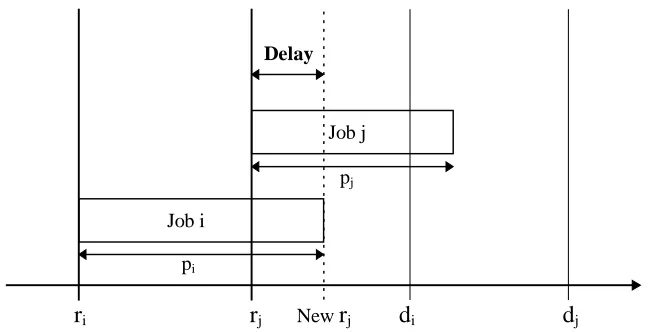
must be processed in release time order. A scenario is depicted in Figure 2.1 where two
jobs on one machine must be completed by their effective due dates. For any job i, di is the
effective due date, ri the effective release time, and pi the processing time.
The conditions of the situation in Figure 2.1 are as follows: (1) release times and due
dates have a specific relational ordering where ri <rj and di <dj, (2) job i cannot finish
exceed its due date, (i.e. rj + pj + pi >di). When all three of these conditions hold, as
depicted in Figure 2.1, the jobs can only be processed in release time order. Thus job j
waits an additional ri + pi - rj time units before it can begin processing (the amount of time job j waits is represented by the double arrow, labeled delay). The release time of job
j can be increased from rj to ri + pi and the effective release times on down-stream machines are increased by a like amount. The effective due dates can also be tightened.
Since job i precedes job j and both jobs must satisfy their respective due dates, job i needs
to finish at least pj time units before dj for job j to be on time. Therefore, di can be reduced
to dj - pj and the up-stream due dates are affected by a like amount.
ri rj New rj di dj
Job i
Job j Delay
pi
pj
Figure 2.1: Example of a Job Forced to be Processed in Release Time Order
This release time order condition is only considered for pairs of adjacent jobs. Extension
to larger job sets would become computationally expensive. As this condition is
the process begins again. This continues until the machines have all been searched without
any changes. At this point, the lower bound can be calculated as done previously, but
with tighter release times and due dates.
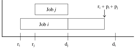
For a second condition that identifies a delay in processing, consider the single machine
graphical example in Figure 2.2a where due dates must be met. This condition is true
when jobs must be processed in due date order instead of release time order. Again, for
any job i, ri is the effective release time, pi the processing time (length of the block), and di
the effective due date. Job i is released but is then preempted so that job j can be
completed by its due date. Although no preemption is assumed, it is used in the lower
bound calculation as a relaxation. Therefore, if a machine is analyzed as if preemption is
not allowed, then job groupings where the sequence is infeasible without preemption can
be identified and adjusted accordingly. For example, Figure 2.2b shows the sequence
change that results from assuming preemption is not allowed in the Figure 2.2a sequence.
In Figure 2.2b, job i must wait for job j to finish before it can begin processing. It is
drawn to demonstrate how job i waits for job j’s completion so that all of job i can be
processed without interruption. The result of this change is that ri is increased to rj + pj and dj is decreased to di - pi. This scenario occurs when the following is true,
ri + pi + pj >dj and (2.1a)
Job i Job j
ri rj dj di
ri + pi + pj
Figure: 2.2a: Example of a Preempted Constrained Sequencing
Job j
Job i
ri rj dj di
rj + pj + pi
Figure 2.2b: Example of a Feasible Constrained Sequencing
The goal is to find a set of jobs in which the sequence used for the lower bound
calculation that allows preemption can be adjusted to reflect a feasible schedule as is
pictorially described in Figures 2.2a and 2.2b. Mathematically, this involves a search for
blocks of processes where inequalities (2.1a) and (2.1b) simultaneously hold true.
To begin this search, the jobs are sequenced in release time order. Then each machine is
investigated separately by looking at all the combinations of two adjacent jobs, three
adjacent jobs, and so forth up to the number of the jobs processed on that machine. Every
job set is checked for feasibility using the inequality (2.1a) stated above. In the general
ri pi j d
j i m
m
+ >
=
∑
, . (2.2)When inequality (2.2) is true for the set of adjacent jobs i through m, job m, the last job in
the set, is tardy, and the current sequencing of the set is infeasible. For job m to meet its
due date, some job in the set i through m-1 must be delayed to begin when job m is
completed. The earliest this delayed job can begin is at time rm + pm.
The second step is the search identifying the job to be delayed until the tardy job is
finished processing. A set of possible candidates is created. First, the options are limited
to the set of adjacent jobs that caused the infeasibility, in the example above jobs i through
m-1. These are the only jobs for which a reordering could decrease the actual start and
finish time of the remaining jobs in the set, (most importantly the tardy job). Second, if a
job is delayed, it must still be completed by its due date. If this is not true, it violates the
basic assumption that in a feasible schedule each job must complete by its due date. This
implies the third requirement that for a job to be a candidate its effective due date must be
greater than that of the tardy job. Since the time that the processing of jobs i through m
ends is greater than job m’s due date, dm, then any job with its due date less than dm will
also not complete on time if it is delayed processing until job m is completed. This
restriction is checked by inequality (2.1b). In the general case where job k is in the set of
ri pi j d
j i m
k
+ ≤
=
∑
, . (2.3)The following three points characterize the necessary conditions for a job to be a
candidate for delay.
Observation 1: The job is in the set of adjacent jobs where the current
ordering forces the last job in the set to be tardy.
Observation 2: The due date of the job is greater than the due date of the
tardy job.
Observation 3: If it is delayed, the job can still completed by its due date.
In choosing the job to delay, the combination of these three observations greatly limits the
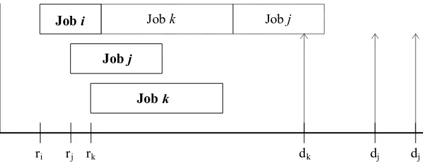
options, but does not necessarily narrow it down to one job. For example, in the graphical
example Figure 2.3a, assume it is known that job k is late when combined with jobs i and j
in release time order. The figure displays a condition such that inequality (2.2),
ri + pi + pj +pk >dk, is true. However, Figures 2.3b and 2.3c demonstrate a condition
such that inequality (2.3) is true for both job i and job j, rj + pj + pk + pi ≤di and
ri + pi + pk + pj ≤dj respectively. Since dj >dk and di >dk, job i and job j are both
ri rj rk dk dj dj Job k
Job j
Job i Job j Job k
Figure 2.3a: Example of Ordering with Multiple Jobs as Options for Delay
Job k Job i
Job k
Job j Job i
ri rj rk dk dj di
epsi
Figure 2.3b: Example of a Reordering where Job i is Delayed
Job k Job j
Job i Job k Job j
ri rj rk dk dj dj
Figure 2.3c: Example of a Reordering where Job j is Delayed
When more than one job can be delayed to compensate for an infeasible ordering, some
standard beyond Observations 1-3 must be used to decide the best choice. To resolve this
lateness is decreased to the point at which only one job can be delayed. Consider what
happens if the UB is decreased. The effective due dates decrease for each job because
they are based on the UB. If the same set of jobs is evaluated again, then at some point,
as the value of the trial lateness is decreased, only one job is left as an option to delay and
still have all jobs meet their due dates. It is possible that two jobs could have identical
release times, processing times, and due dates. If this occurs either job can be delayed to
obtain a feasible sequence.
For each delay candidate the specific amount of UB decrease is found. When a candidate
job is delayed processing until after the tardy job, the tardy job is then processed and
finished earlier. The amount of decrease for a candidate job is determined by how much
earlier the tardy job will actually finish if that specific candidate job is delayed. This
amount will often be simply the candidate job’s processing time, pc. It can however be
less than pc because a job can exist between the candidate job and the tardy job whose
earliest start time does not allow it to begin pc units earlier. Thus, each job candidate has
an effective processing time, epsc, that represents how many time units earlier the tardy job
begins when a job candidate is delayed. In Figure 2.3b, job i’s effective processing time,
epsi is shown; it does not equal pi because when job i is delayed, job k only begins epsi units earlier instead of pi units earlier. The value of a candidate job candidate depends on
how much the tardy job gains from its delay, epsc, compared to the slack on the delayed
job candidate with the maximum value is the job that will be delayed; its value is the
amount of reduction required to eliminate all the other candidates.
In summary, a job is found to be tardy when processed at the end of a block, in response
some job in the block must be delayed. The options are narrowed down by using the three
observations stated earlier and reducing the trial lateness until only one job remains as a
feasible option.
Once the job to be delayed is found, updates in the effective release times and due dates
must be made accordingly. First, the effective release time of the job delayed is increased
to the time when the tardy job is finished. For example, if job m is tardy and job k is
delayed until job m is finished, then the effective release time for job k, rk, is increased to rm
+ pm. Along with that increase, the effective release times for job k “down-stream” of the current operation are also increased by the same amount, rm + pm - rk. Although the due dates are affected less frequently, they can also be tightened to reflect the change in order.
In the example notation, since job k must satisfy its due date and job m now precedes it,
job m must be finished by dk - pk to allow job k to be completed on time. Therefore, job
m’s due date, dm, becomes the minimum of dm and dk - pk.
The situation just discussed assumes that when jobs begin in release time order, using the
trial lateness to search for infeasible orderings will result in the identification of at least
Mathematically, this means that inequality (2.2) is initially false for each set of adjacent
jobs on every machine.
This scenario occurs when the difference between the upper bound and the lower bound is
large. When this gap is large, the effective due dates and effective release times are
conservative, making a tardy job a rare find. However, as trial lateness values are tested
(i.e., the UB is decreased), finding a tardy job becomes much more likely. When an
infeasible ordering is found effective release times are increased. Then, the number of
identifiable infeasible orderings will often grow linearly as the effective down-stream
release times are increased.
The procedure for finding the trial lateness value to test is essentially identical to that of
choosing which job to delay just described for when multiple candidates exist. Consider
the results when the UB is decreased one unit at a time. After each decrease, the
up-stream due dates are recalculated for each machine. At some point, as the effective due
dates decrease, at least one inequality of type (2.2) will be true. The machine that contains
this set of jobs, the set in which the order causes one job to be tardy, is the “Lmax
machine”, that is, the machine that has the largest Lmax when the lower bound is calculated.
This machine is now the focus for finding the new trial lateness. The point where
inequality (2.2) becomes true can be found using the slack on the inequalities.
forces the last job in the set tardy, in other words an instance when inequality (2.2)
becomes true. Therefore, all the slack values are calculated once, and as stated below in
Observation 4, the minimum of these values is the exact amount that the trial lateness is
decreased to obtain at least one instance where inequality (2.2) is true. From here, the
procedure is the same as when finding an infeasible ordering in the initial search. The only
difference is that now the set of jobs to reorder is known.
At this point the trial lateness has been identified as a specific value based on slack. If this
trial lateness is possible then some job must be delayed. The job will come from the set of
jobs that caused the decreased value. As discussed in detail earlier, the trial lateness is
reduced further yet to the point where only one job can be delayed. To test for stopping
the procedure, the trial lateness that was used to choose the job set and the further
reduced lateness to choose the delayed job are both considered. The stopping procedure
will be discussed next.
Observation 4: The minimum slack is the amount the trial lateness can be
reduced before at least one feasibility inequality becomes true.
Decreasing the trial lateness will often result in an increase in the lower bound. With each
trial lateness value, the schedule is checked to see if a reordering can compensate for the
due dates that result from the reductions. If possible, the appropriate adjustments are
times. The process stops when either the bounds meet, cross, or when no feasible change
in order exists to satisfy the due dates corresponding to the trial lateness. The bounds will
meet or cross when the trial lateness is pushed down, and the resulting lower bound
calculation jumps up to or above it. The trial lateness quantity that is considered includes
the additional amount it is reduced in choosing just one job to be delayed.
Stopping the procedure can become difficult because of the downstream effects of
increasing release times. Once a change is made and the effective release times are
updated, the procedure repeats and searches for the next trial lateness. Because Lmax may
increase on some downstream machines, it is possible for the next trial lateness to be
larger than the previous one. In fact, a typical pattern for the trial lateness values is one
that gradually decreases with a few small increases in between. Throughout the
procedure, the minimum trial lateness that has been tested is kept as the standard for
stopping. As a conservative stopping rule, if the LB goes up while the current trial
lateness is not at its minimum, the process stops.
The steps of the algorithm to improve the lower bound are as follows.
1. Read in job release times, due dates, and routings.
2. Calculate earliest start and latest finish times.
3. Check for adjacent jobs that must be processed in release time order as in Figure 2.1
b) di < dj
c) ri + pi > rj
d) rj + pj + pi > di
4. If two jobs are found to always be in release time order, they meet the conditions in
the above step, update rj to max{rj, ri+pi}, and di to min{di, dj-pj}. Go Back to step 2.
5. Set k=1.
6. On machine k:
a) Get effective release times and due dates.
b) Place jobs in release time order.
c) Calculate Lmax for blocks of adjacent jobs. Blocks of size 2, 3, etc.
d) Save, the largest Lmax on a block as the Lmax value for machine k, and the block
on which it occurred. If a tie exists between blocks, use the smallest block.
e) (If the UB is reduced by the Lmax value for the block, the last job will be tardy.)
Using Observations 1-3, find the jobs that can be delayed until after the tardy
job so that all the jobs meet their due dates that have been reduced by the
amount of the block Lmax.
f) If more than one job can be delayed, find the specific job by which job is left as
a feasible option if the due dates are reduced further. Save the value of this
further reduced UB.
g) Save the release time and due date changes that occur from the delay.
7. Increase k to k+1.
9. Choose the machine with the largest Lmax value and update the release time and due
date that correspond to the delay found for that machine.
10. Recalculate the overall earliest start times, latest finish times, and the lower bound.
11. Compare the new lower bound (NLB) to the reduced trial lateness (RTL) value used
to decide which job to delay.
a) If NLB = RTL, the lower bound stands.
b) If NLB > RTL, the previous lower bound value is the lower bound.
c) If NLB < RTL, go back to step 3.
3. An Example Problem
As an example, refer to the problem from Sundaram and Fu [15], Palmer [12] shown in
Table 3.1 and Figure 3.1. Step 1: read in the release time, due dates, and processing times
from Table 3.1. Step 2: calculate the earliest start and latest finish for each operation of
each job. Although this is originally a makespan problem, it can be considered an Lmax
problem with the same due date of 100 for each job. From the original due dates of 100,
the effective due dates (earliest starts) are calculated. For example, job 1 has four
operations and is due at time 100. Since job 1, operation 4 takes 3 units to process, the
upstream operation of job 1, operation 3, has an effective due date of 97. The effective
release times are found in a similar manner. Each job is released at time 0 and its second
operation is simply zero plus the processing time of the first operation. For example, job
operation 2 has a release time of 5. This continues on in the same manner for the
remainder of the jobs.
Table 3.1: Example Problem from Sundaram and Fu, Palmer
JOB OPERATION MACHINE PROCESSING
TIME
RELEASE TIME
DUE-DATE
one 1 m1 5 0 84
2 m2 7 5 91
3 m3 6 12 97
4 m4 3 18 100
two 1 m1 7 0 79
2 m2 4 7 83
3 m3 7 11 90
4 m5 10 18 100
three 1 m2 4 0 85
2 m4 5 4 90
3 m4 6 9 96
4 m5 4 15 100
four 1 m2 2 0 82
2 m3 8 2 90
3 m3 3 10 93
4 m4 7 13 100
five 1 m1 3 0 84
2 m3 7 3 91
3 m5 6 10 97
4 m5 3 19 100
Step 3: the jobs are checked for the first condition described in the previous section when
only two adjacent jobs are considered at a time. For example on machine 1, the release
times are all the same, so right away no jobs fit the condition ri < rj. On machine 2, job 4 is
released before job 1 and is then due before job 1. Therefore the first two constraints that
r4 < r1 and d4 < d1 are true. The next condition that r4 + p4 > r1 is not true. At this point in
the problem no two jobs will initially meet the fourth criterion. Therefore, step 4 is
skipped. Even if two jobs do exist that meet these first three constraints, because the due
condition did happen to be satisfied, the process would begin again with the updated
earliest starts and latest finishes.
M5 M4 M3 M2 M1 40 35 30 25 20 15 10 5 1 5 4’ 4
4 5 4’ 1
3 3’ 2 4 1
3 3’ 2 4 1 2 5 1
1 5 2
3 4 1 2 1 2 4 3 5 3 2 5’ 5’
5 3 2
Figure 3.1: Gantt Chart of Initial Sequencing of the Example Problem
processing lengths at the moment they are released. The second grouping shows the jobs
as they are actually processed when in the initial sequence.
Next, each set of adjacent jobs is checked for feasibility using inequality 2.2. Step 6c: Lmax
is found on every machine. Step 6d: the maximum of these machine Lmax’s is the amount
the upper bound (trial lateness) is reduced if no job sets are initially found infeasible.
Beyond this calculation is the additional amount the trial lateness must be reduced to
actually make the change in ordering. That is, step 6e&f: when more than one job can be
delayed to correct an infeasible ordering and the trial lateness must be further reduced to
make the decision.
In the example, it is obvious that every job will be finished processing by its effective due
date. Therefore, Lmax is calculated for each machine to determine how much to reduce
the trial lateness. On machine 1 the current job order gives the following finished
processing times: for two jobs, r1 + p1 + p5 = 8 with d5 = 84, therefore Lmax = 8-84 = -76.
Also for two jobs r5 + p5 + p2 = 10 with d2 = 79, therefore Lmax = 10-79 = -69; for three
jobs, r1 + p1 + p5 + p2 = 15 with d2 = 79, but here two jobs remain as options to be delayed. Therefore, Lmax = 15-79 = -64, but there is an additional reduction for the
decision between options. This reduction is the max{min(p1,d1-d2),min(p5,d5-d2)} = max{min(5,5),min(3,5)} = 5 and therefore the trial lateness for that block is -64-5 = -69.
Since the 5 corresponds to job 1, it is the job chosen to delay until job 2 is completed.
and 2 on machine 1 provide the maximum of the Lmax’s at -64. The overall due dates are
adjusted by the largest Lmax, -64, thus job 1 is forced to delay. At this time the precedent
constraint that on machine 1 job 1 must precede job 2 is established.
Finally, the change in order and its effects must be implemented. Step 9: since on machine
1, job 1 must wait for job 2, then job 1’s release time is changed to the maximum of its
original release time, r1 = 0, and the earliest time that job 2 can finish is r2 + p2 = 0 + 7 = 7. This increase of seven is then added to all of job 1’s down-stream operations. For
example, job 1, operation 2’s former release time of 5 is now 12. Also, job 2’s due date
may be updated. Since on machine 1 job 2 must precede job 1, job 2 must be finished in
time for job 1 to be completed before its due date. Therefore, d2 becomes the minimum of
its original value and d1-p1. Step 10: the process repeats as the lower bound is again calculated, but now with more accurate release times. Step 11: if the new lower bound
has not reached the trial lateness, another reduction in the trial lateness is made. Effective
release times are updated down-stream to reflect the delay; the effective due dates (latest
finishes) must also be updated. For example, job 2, operation 1’s effective due date is
now 79-64 = 15.
When the procedure is completed, the lower bound may have increased, but beyond that
calculation, release times and due dates are more accurate and some precedence relations
lateness at or below the trial lateness value. Release times, due dates, and precedence
constraints are all updated at each trial lateness allowing this information to be used at
each iteration of the decreasing bound.
4. Summary
In summary, the procedure begins with a known upper bound lateness as the trial lateness.
This value is a known lateness to the problem. Because the UB is reduced to a value that
is dependent on the problem, the starting UB is not important to the procedure. The
lower bound (LB) value is repeatedly calculated after every order change by allowing
preemption on all but one machine at a time. To improve the LB, a search is done to
identify partial orderings that must hold in order to meet the trial lateness. First sets of
two jobs that must be processed in release time order, then blocks of jobs that must be
processed in due date order. This is one way of replacing the preemption relaxation with
machine idle time in the LB calculation. The trial lateness is then tested at specific lower
values. The decisions become what new trial lateness to use and what partial ordering in
needed to achieve this lateness.
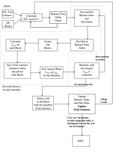
The flowchart in Figure 4.1 shows a precise summary of how the lower bound
improvement is implemented. As stated before, it begins with two inputs: a known UB as
the first trial lateness, and the machines at which the operations of each job are performed
1RPDFKLQHVDUHOHIW.
Delay a Job in the Block with the Smallest
Trial Lateness
Update Release Times and Due Dates.
Update Trial Lateness. Calculate
ES’s and LF’s. Inputs UB -Trial Lateness Job Routes Get machine Release times and Due Dates
Put Jobs in Release Time
Order Calculate
Lmax on each Block
Save Trial Lateness needed to delay
one job for each Block
Save largest Block Lmax as Lmax for the Machine
Machine with the Largest
Lmax is
evaluated
0RUHPDFKLQHV WRSURFHVV
,I/%≥PLQWULDOODWHQHVV QRRUGHUFKDQJHZDVPDGHRU WULDOODWHQHVV!PLQWULDOODWHDQG WKH/%LQFUHDVHG END FKDQJH LQRUGHU
Get trial lateness on each machine
found for each operation on each job. The release time order check is done first and it
starts over each time a change is made. The process then investigates the due date order
condition. Machines are evaluated one at a time, but no changes are made until all the
machines are checked. Release times and due dates are calculated for the machine under
consideration, and the jobs are arranged in release time order. The jobs begin this way for
every iteration of the procedure, but as partial order changes are established, the
corresponding release times will be updated to reflect the changes. Next, blocks are
formed. Then Lmax and a trial lateness is found for each block. The details of this
calculation are described next.
While still looking at just one machine, each set of adjacent jobs is checked beginning with
sets of 2, 3,and up to the number of jobs on the machine. For each of these sets the
lateness of the last job is found. If a job is found to be tardy, then some job in that set is
delayed so that all the jobs finish by their respective due dates. To identify this delayed
job, the trial lateness is decreased until a decision can be made. Thus, each set of adjacent
jobs has a trial lateness value that includes the amount of decrease that is required to force
reordering. The block trial lateness is now an option for the next overall trial lateness.
Across the blocks on the machine, the largest of the possible trial lateness is saved. The
procedure repeats and each machine is evaluated in this way. Then on the machine with
Finally, the machine, the tardy job, and the delayed job that all correspond to the new trial
lateness are updated accordingly. A partial ordering is established where the tardy job, to
be on time, must proceed the delayed job on that machine. Therefore, a precedent
constraint is established and available for later use. Also, the effective release times of the
delayed job are increased to reflect the delay; and the due dates of the tardy job are
updated to reflect the delayed job’s new position. Once these changes are made, the
procedure starts over beginning with recalculation of earliest starts and latest finishes.
5. Experimental Results
The procedure described above was implemented in Fortran, (the code is provided in
Appendix B). Demirko, Mehta, and Uzsoy [6] generated job shop scheduling problems
that are used as a standard for half of the tests. “For problems with Lmax as a performance
measure, due dates are determined using two parameters, T and R. T determines the
expected number of tardy jobs (and hence the tightness of the due dates), and R is the due
date range parameter. The job due dates are generated from a distribution, Uniform[µ
-µR/2, µ+µR/2], where µ=(1-T)nP”. P is the average processing time, here 100.5, and n is
the varying number of jobs. The procedure was tested on 160 of these problems and the
results are shown in Appendix A. The problems are defined by N_M_t_r_problem#,
where t=1 when T=0.3, t=2 when T=0.6, r=1 when R=0.5, and r=2 when R=2.5. Table
A.1 displays the problems with 20 jobs on both 15 and 20 machines. The columns
but for problems with 30, 40, and 50 jobs. The problems are grouped with 5 problems at
each N_M_t_r level. Scanning the four tables, it is obvious that most of the increases in
the lower bound are on the problems with r=2. Of the 26 improvements, 24 are accounted
for by problems where r=2. From this sample of data it appears that the larger the range,
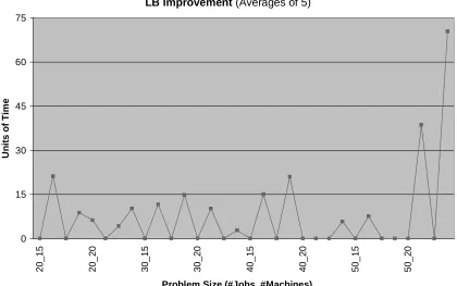
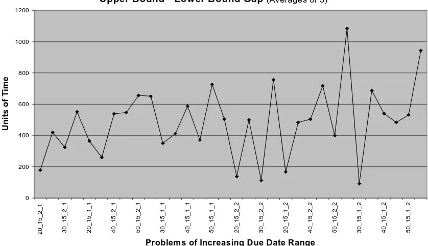
the lower bound increases more frequently. Figures 5.1, and 5.2 emphasize this point.
Figure 5.1 simply shows the LB increases as the problem size increases. Figure 5.2
contains the same information, but it is arranged in order of increasing due date ranges to
demonstrate that more improvements occur at the larger ranges. However, this may not
be the only explanation, as Figure 5.3 demonstrates. Here, the gap between the upper
Uzsoy’s Problems LB Improvement (Averages of 5)
0 15 30 45 60 75
20_15 20_20 30_15 30_20 40_15 40_20 50_15 50_20
Problem Size (#Jobs_#Machines)
U
n
it
s of Ti
m
e
Uzsoy’s Problems
LB Improvements (Averages of 5)
0 15 30 45 60 75
20_15_2_1 30_15_2_1 20_15_1_1 40_15_2_1 50_15_2_1 30_15_1_1 40_15_1_1 50_15_1_1 20_15_2_2 30_15_2_2 20_15_1_2 40_15_2_2 50_15_2_2 30_15_1_2 40_15_1_2 50_15_1_2
Problems of Increasing Due Date Range
Units of Time
Figure 5.2: Lower Bound Improvements Arranged by Increasing Due Date Ranges
Uzsoy’s Problems
Upper Bound - Lower BoundGap (Averages of 5)
0 200 400 600 800 1000 1200
U
n
it
s of
Ti
m
bound and the old lower bound is displayed as the due date range increases. There is a
general tend toward a larger gap between the bounds at larger due date ranges that may
also contribute to why more improvements exist at the larger ranges.
The second set of problems are slightly different in that the due date range is what
distinguishes the problems. Consider the solution to an Lmax problem. If constants were
added to each of the due dates more jobs would be tardy, but the solution schedule would
not change. As defined for the previous problems, the parameter T determines the
expected number of tardy jobs. Thus, the important descriptive parameter of due dates is
the range. Also, Demirkol, Mehta, and Uzsoy’s problems assume that each job is
processed on every machine, (i.e. number of machines equals the number of operations per
job). This second set of problems reflect industrial scenarios where jobs have only a few
operations relative to the number of machines. The processing times were generated from
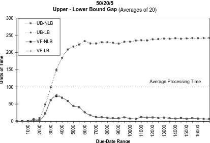
a uniform distribution , U[1,200], (average processing time of 100.5). Figure 5.4, shows
the problems with 50 jobs, 20 machines, and 5 operations per job. At each due date range
20 problems were tested. As Figure 5.4 displays, only three problems had an
improvement in the lower bound. However, the improvements that were made are critical
because of their location along the due date range. Figure 5.5 depicts the gap between the
upper bound and lower bound for the same problems. The chart includes upper bound
solutions from a scheduling heuristic by Hodgson, Cormier, Weintraub and Zozom [9],
referred to as the Virtual Factory (VF). The four lines are: the UB-NLB, (a conservative
minus the previous lower bound), virt-LB, (an enhanced VF solution minus the previous
lower bound), and virt-LB, (the same improved upper bound minus the improved lower
bound). Each data point is the average of the 20 problems at the specified due date range.
The enhanced VF solution shows that the gap between the bounds is essentially zero
except for a small range of due dates in the middle. This is the exact location of the
increases in the lower bound.
Another advantage of the improved lower bound is that the variance of each point
(average of 20 problems) is reduced. For example, at the due date range of 3000, the
average gap was reduced from 76.6 to 72.5 and the variance reduced from 65.0 to 57.0.
Figures 5.6 and 5.7, 5.8 and 5.9, and 5.10 and 5.11 show the same type of observations as
Figures 5.4 and 5.5 for different sized problems. In each set of graphs, it is clear that the
lower bound improvements occur at the critical point along the range.
An increased lower bound makes any N/M/Lmax job shop scheduling heuristic appear
more efficient. There is also additional information that can be extracted from the lower
bound procedure that may be useful as input to improve an actual schedule. The lower
bound improvement process identifies partial orderings that must be enforced for the
particular trial lateness at that iteration to be achieved.. These partial orderings can also
50/20/5 LB Improvements 0 10 20 30 40 50 60 0
1000 2000 3000 4000 5000 6000 7000 8000 9000
10000 11000 12000 13000 14000 15000 16000
Due-Date Range U n it s of Ti m e
Figure 5.4: Lower Bound Improvements in 50/20/5 Size Problems
50/20/5
Upper - Lower Bound Gap (Averages of 20)
0 50 100 150 200 250 300
1000 2000 3000 4000 5000 6000 7000 8000 9000
10000 11000 12000 13000 14000 15000 16000
Due-Date Range
U
n
it
s of Ti
m e UB-NLB UB-LB VF-NLB VF-LB
Average Processing Time
100/20/5 LB Improvements
0 5 10 15 20 25 30 35
0
1000 2000 3000 4000 5000 6000 7000 8000 9000
10000 11000 12000 13000 14000 15000 16000 17000
Due-Date Range
U
n
it
s of
Ti
m
e
Figure 5.6: Lower Bound Improvements for 100/20/5 Size Problems
100/20/5
Upper - Lower Bound Gap (Averages of 20)
0 50 100 150 200 250 300
1000 2000 3000 4000 5000 6000 7000 8000 9000
Uni
ts of
Ti
m
e
UB-NLB
UB-LB
VF-NLB
VF-LB
100/10/5 LB Improvements 0 20 40 60 80 100 120 140 160 180 0
1000 2000 3000 4000 5000 6000 7000 8000 9000
10000 11000 12000 13000 14000 15000 16000 17000
Due Date Range
U n it s of Ti m e
Figure 5.8: Lower Bound Improvements for 100/10/5 Size Problems
100/10/5
Upper - Lower Bound Gap (Averages of 20)
0 50 100 150 200 250 0
1000 2000 3000 4000 5000 6000 7000 8000 9000
10000 11000 12000 13000 14000 15000 16000 17000
Due Date Range
U
n
it
s of Ti
m e UB-NLB UB-LB VF-NLB VF-LB
Average Processing Time
500/100/10 LB Improvements
0 20 40 60 80 100 120 140
0
1000 2000 3000 4000 5000 6000 7000 8000 9000 10000 11000 12000 13000 14000 15000 16000
Due-Date Range
Units of Time
Figure 5.10: Lower Bound Improvements in 500/100/10 Size Problems
500/100/10
Upper - Lower Bound Gap (Averages of 20)
0 50 100 150 200 250 300 350 400 450 500
0
1000 2000 3000 4000 5000 6000 7000 8000 9000
U
n
it
s of Ti
m
e
UB-NLB
UB-LB
VF-NLB
VF-LB
The precedence constraints were used as input for Hodgson, Cormier, Weintraub and
Zozom’s VF [9]. The VF is a simulation-based approach to sequencing jobs in a large
job shops. With Lmax as the criterion, it iteratively uses the queueing time for each job at
each machine to update the operation’s release time. The jobs are sequenced according
to a slack calculation and are then reordered as the release times change. As described in
detail in the previous section, the lower bound improvements are a result of enforced
order changes. These are recorded as precedence constraints and made available as input
to the VF. These precedence constraints may force machine idle time. Before a job is
scheduled a check is run to make sure all the required preceding jobs are completed. If
no job can be processed, the machine sits idle causing additional queueing time for those
jobs waiting.
A precedent constraint is made under the condition that if a schedule is able to yield the
trial lateness under consideration then that constraint must hold. With each new trial
lateness value tested an additional precedent constraint is formed. However, all of the
constraints from all the trial lateness values may not be used as input to the simulation.
This is the case because the problem may not actually be able to reach as low an Lmax value
as was used in the testing procedure to improve the lower bound. Thus, the exact number
of precedent constraints to use in the simulation is unknown. To accommodate this fact,
VF was run multiple times for each problem with an additional constraint added each at
run. The constraints were added in the order from which they were extracted from the
solutions tended to bounce up and down usually hitting a minimum within the first 15 to
20 runs regardless of the number of total runs.
The results of the Virtual Factory (VF) tests are shown in Tables A.5-A.8. The columns
represent respectively: the problem identifier, the previous best known upper bound (UB),
the original VF UB solution, the VF UB with the additional precedence input, the
percentage of the gap decreased between the original VF UB solution and the VF UB
solution with precedence constraints, and the percentage of the gap decreased between the
best known UB and the VF UB with precedence constraints. When the precedence
information is used, an improvement in the VF is evident for about 85% of the problems
tested. Consistent with the lower bound improvements, the best known UB was improved
upon for a number of the problems with R = 2.5. On these problems 69% of the previous
best UB was improved on by the VF using the precedence input while less than 1% where
improved when R = 0.5.
6. Conclusions and Further Research
Looking at the results, the impact obviously affects specific groups of problems. An area
to study further is why particular problems had a significant improvement in the lower and
upper bounds and others had virtually no improvement. What characteristics do these
particular problems have in common that allow delays to be identified? Do the problems
idle time and orderings that are assumed but not counted in this procedure. Answers to
these and similar questions could provide insight into areas of potential lower and upper
bound improvements.
Besides the partial orderings described by the precedence constraints other valuable
information is available from the lower bound calculation. Along with every precedence
constraint an updated earliest start and latest finish is calculated. These values could be
used as input instead of the precedence information or in addition to it. In using both
precedence constraints and earliest starts/latest finishes, redundancy is a relevant issue to
consider. Because the Lmax scheduling problem is solved in such a variety of ways, the
information resulting from the lower bound has numerous possibilities as input depending
on the heuristic.
Further research concerning the lower bound could also encompass the application to
industrial size problems. The current procedure assumes one machine exists for each type
of operation. A realistic extension would include identical machines that perform the same
References
[1] Applegate, D., and W. Cook, “A Computational Study of the Job-Shop Scheduling Problem,” ORSA Journal on Computing, 3, 2, pp. 149-156, 1991.
[2] Bratley, P., M. Florian, and P. Robillard, “Scheduling with Earliest Start and Due Date Constraints,” Navel Research Logistics Quarterly 18, pp. 511-517, 1971.
[3] Brucker, P., and B. Jurisch, “A New Lower Bound for the Job-Shop Scheduling Problem,” European Journal of Operational Research, 64, pp. 156-167, 1993.
[4] Carlier, J., “The One-Machine Sequencing Problem,” European Journal of
Operational Research, 11, pp. 42-47, 1982.
[5] Carlier, J., and E. Pinson, “An Algorithm for Solving the Job Shop Problem,”
Management Science, 35, 2, pp. 164-176, 1989
[6] Demirkol, E., S. Mehta, and R. Uzsoy, “Benchmarks for Shop Scheduling Problems,” Research Memorandum No. 96-4, School of Industrial Engineering, Purdue University, West Lafayette, IN 47907.
[7] Dogramaci, A., and J. Surkis, “Evaluation of a Heuristic for Scheduling Independent Jobs on Parallel Identical Processors,” Management Science, 25, 12, pp. 1208-1216, 1979.
[8] Garey, M., and Johnson, D. Computers and Intractability: A Guide to the Theory
of NP Completeness. W.H. Freeman, San Francisco, 1979.
[9] Hodgson, T. J., D. Cormier, A. J. Weintraub, and A. Zozom, Jr., “Satisfying Due-Dates in Large Job Shops,” to appear Management Science.
[10] McMahon, G., and M. Florian, “On Scheduling with Ready Times and Due Dates to Minimize Maximum Lateness,” Operations Research, 23, 3, pp. 475-482, 1974.
[11] Ovacik, I., and Uzsoy, R. “Decomposition Methods for Scheduling Semi-Conductor Testing Facilities,” International Journal of Flexible Manufacturing Systems, 8, pp. 357-388.
[14] Slotnick, S., and T. E. Morton, “Selecting Jobs for a Heavily Loaded Shop with Lateness Penalties,” Computers and Operations Research, 23, 2, pp.131-140, 1996.
[15] Sundaram, R. M., and S.-S. Fu, “Process Planning and Scheduling - A Method of Integration for Productivity Improvement,” Computers and Industrial Engineering,
Table A.1: LB Improvement in Uzsoy’s 20 job Problems
Problem LB NLB LB Increase UB
20_15_1_1_6 1027 1027 0 1448
20_15_1_1_8 1127 1127 0 1552
20_15_1_1_4 1160 1160 0 1492
20_15_1_1_2 1140 1140 0 1464
20_15_1_1_3 1182 1182 0 1501
20_15_1_2_1 1769 1721 0 2090
20_15_1_2_10 1775 1839 64 2067
20_15_1_2_9 1956 1956 0 2246
20_15_1_2_5 1925 1967 42 2135
20_15_1_2_8 1599 1575 0 1785
20_15_2_1_7 1575 1575 0 1975
20_15_2_1_3 1727 1727 0 2100
20_15_2_1_1 1785 1785 0 2165
20_15_2_1_5 1521 1521 0 1839
20_15_2_1_9 1858 1858 0 2143
20_15_2_2_10 1282 1282 0 1682
20_15_2_2_2 1688 1619 0 2159
20_15_2_2_3 1894 1894 0 2381
20_15_2_2_7 1596 1640 44 1943
20_15_2_2_4 1663 1663 0 2018
20_20_1_1_7 1391 1386 0 2013
20_20_1_1_10 1182 1213 31 1708
20_20_1_1_6 1366 1366 0 1962
20_20_1_1_3 1569 1569 0 2235
20_20_1_1_4 1226 1226 0 1753
20_20_1_2_9 2147 2147 0 2631
20_20_1_2_6 2376 2362 0 2842
20_20_1_2_2 2106 2106 0 2458
20_20_1_2_4 2469 2469 0 2689
20_20_1_2_8 2378 2378 0 2712
20_20_2_1_2 1776 1797 21 2638
20_20_2_1_6 1868 1868 0 2586
20_20_2_1_4 1845 1845 0 2535
20_20_2_1_8 1927 1927 0 2599
20_20_2_1_7 1947 1947 0 2640
20_20_2_2_1 1982 1972 0 2552
Table A.2: LB Improvement in Uzsoy’s 30 job Problems
Problem LB NLB LB Increase UB
30_15_1_1_10 1185 1185 0 1379
30_15_1_1_7 1263 1263 0 1459
30_15_1_1_6 1255 1255 0 1441
30_15_1_1_5 1205 1205 0 1360
30_15_1_1_9 1320 1320 0 1483
30_15_1_2_10 2240 2263 23 2696
30_15_1_2_2 2436 2427 0 2891
30_15_1_2_3 1935 1936 1 2296
30_15_1_2_5 2475 2459 0 2940
30_15_1_2_8 2169 2203 34 2531
30_15_2_1_8 2252 2252 0 2750
30_15_2_1_1 2042 2042 0 2347
30_15_2_1_3 2189 2189 0 2470
30_15_2_1_9 2224 2224 0 2496
30_15_2_1_4 2401 2401 0 2666
30_15_2_2_6 1734 1734 0 2433
30_15_2_2_3 2068 2113 45 2678
30_15_2_2_5 1960 1989 29 2515
30_15_2_2_9 1922 1922 0 2380
30_15_2_2_7 2075 2075 0 2510
30_20_1_1_3 1268 1268 0 1816
30_20_1_1_6 1412 1412 0 1952
30_20_1_1_2 1575 1575 0 2173
30_20_1_1_9 1710 1710 0 2237
30_20_1_1_1 1611 1611 0 2094
30_20_1_2_9 2314 2314 0 2979
30_20_1_2_8 2713 2764 51 3418
30_20_1_2_7 2817 2817 0 3312
30_20_1_2_2 2386 2366 0 3021
30_20_1_2_5 2292 2292 0 2523
30_20_2_1_2 2178 2178 0 2953
30_20_2_1_3 2298 2298 0 3032
30_20_2_1_6 2461 2461 0 3114
30_20_2_1_10 2496 2496 0 3074
30_20_2_1_7 2562 2562 0 3104
30_20_2_2_4 2061 2067 6 2762
30_20_2_2_2 2254 2254 0 2975
30_20_2_2_5 2485 2485 0 3244
30_20_2_2_10 2570 2570 0 3112
Table A.3: LB Improvement in Uzsoy’s 40 job Problems
Problem LB NLB LB Increase UB
40_15_1_1_3 1191 1191 0 1431
40_15_1_1_8 1533 1533 0 1787
40_15_1_1_1 1299 1299 0 1468
40_15_1_1_4 1542 1542 0 1648
40_15_1_1_10 1460 1460 0 1527
40_15_1_2_3 1563 1615 52 2119
40_15_1_2_10 1669 1651 0 2377
40_15_1_2_5 1545 1568 23 2022
40_15_1_2_6 1695 1678 0 2125
40_15_1_2_7 1936 1936 0 2187
40_15_2_1_9 2893 2893 0 3093
40_15_2_1_2 2815 2815 0 2894
40_15_2_1_10 3048 3048 0 3120
40_15_2_1_6 2818 2818 0 2875
40_15_2_1_8 2878 2878 0 2924
40_15_2_2_2 2125 2125 0 2984
40_15_2_2_1 1836 1941 105 2524
40_15_2_2_10 1896 1896 0 2539
40_15_2_2_6 2119 2119 0 2767
40_15_2_2_3 2038 2038 0 2633
40_20_1_1_1 1395 1395 0 2058
40_20_1_1_4 1597 1597 0 2332
40_20_1_1_2 1640 1640 0 2143
40_20_1_1_10 1411 1411 0 1834
40_20_1_1_6 1835 1835 0 2212
40_20_1_2_4 2610 2607 0 3104
40_20_1_2_3 2964 2935 0 3457
40_20_1_2_2 2798 2794 0 3227
40_20_1_2_9 3059 3059 0 3532
40_20_1_2_8 2441 2388 0 2967
40_20_2_1_1 2827 2827 0 3430
40_20_2_1_8 3113 3113 0 3691
40_20_2_1_4 2843 2843 0 3366
40_20_2_1_3 3025 3025 0 3572
40_20_2_1_5 3129 3129 0 3535
40_20_2_2_5 2687 2687 0 3951
Table A.4: LB Improvement in Uzsoy’s 50 job Problems
Problem LB NLB LB Increase UB
50_15_1_1_7 1050 1050 0 1419
50_15_1_1_5 1418 1418 0 1545
50_15_1_1_8 1957 1957 0 2042
50_15_1_1_4 1707 1707 0 1764
50_15_1_1_9 1757 1757 0 1804
50_15_1_2_8 2217 2200 0 2758
50_15_1_2_1 2284 2284 0 2673
50_15_1_2_7 2192 2230 38 2753
50_15_1_2_4 2085 2085 0 2621
50_15_1_2_2 2137 2137 0 2609
50_15_2_1_5 3216 3216 0 3492
50_15_2_1_8 3391 3391 0 3525
50_15_2_1_9 3396 3396 0 3466
50_15_2_1_2 3181 3181 0 3220
50_15_2_1_4 3277 3277 0 3316
50_15_2_2_9 2323 2323 0 3203
50_15_2_2_7 2464 2464 0 3295
50_15_2_2_5 2381 2381 0 2966
50_15_2_2_10 2345 2345 0 3130
50_15_2_2_6 2486 2486 0 3184
50_20_1_1_5 1591 1591 0 2181
50_20_1_1_3 1746 1746 0 2390
50_20_1_1_2 1794 1794 0 2355
50_20_1_1_6 1845 1845 0 2219
50_20_1_1_4 1786 1786 0 2142
50_20_1_2_6 2363 2446 83 3222
50_20_1_2_2 2440 2547 107 3049
50_20_1_2_10 2824 2824 0 3576
50_20_1_2_8 2918 2921 3 3657
50_20_1_2_5 3205 3205 0 3833
50_20_2_1_2 3189 3189 0 3788
50_20_2_1_5 3419 3419 0 3875
50_20_2_1_10 3407 3407 0 3789
50_20_2_1_7 3642 3642 0 3971
50_20_2_1_4 3527 3527 0 3758
50_20_2_2_10 2628 2801 173 3768
50_20_2_2_5 2774 2774 0 3932
50_20_2_2_1 2500 2534 34 3614
50_20_2_2_8 2472 2617 145 3588
Table A.5: Precedent Constrained Solutions for T = 0.3 and R= 0.5
N_M Problem Previous
UB
VF UB VF with
Prec.
%Improve on VF
%Improve Prec. UB
20_15 1_1_2 1464 1596 1546 11% 0%
1_1_3 1501 1591 1562 7% 0%
1_1_4 1492 1614 1614 0% 0%
1_1_6 1448 1511 1474 10% 0%
1_1_8 1552 1687 1687 0% 0%
20_20 1_1_10 1708 1843 1843 0% 0%
1_1_3 2235 2235 2235 0% 0%
1_1_4 1753 1832 1823 2% 0%
1_1_6 1962 2050 2002 10% 0%
1_1_7 2013 2167 2104 8% 0%
30_15 1_1_10 1379 1659 1659 0% 0%
1_1_5 1360 1577 1524 17% 0%
1_1_6 1441 1655 1628 7% 0%
1_1_7 1459 1590 1532 18% 0%
1_1_9 1483 1791 1683 23% 0%
30_20 1_1_1 2094 2197 2163 6% 0%
1_1_2 2173 2417 2414 0% 0%
1_1_3 1816 2028 1981 10% 0%
1_1_6 1952 2062 1985 22% 0%
1_1_9 2237 2297 2240 10% 0%
40_15 1_1_1 1468 1777 1735 9% 0%
1_1_10 1527 1656 1623 27% 0%
1_1_3 1431 1672 1645 7% 0%
1_1_4 1648 1880 1837 13% 0%
1_1_8 1787 2046 1910 27% 0%
40_20 1_1_1 2058 2262 2262 0% 0%
1_1_10 1834 2281 2261 3% 0%
1_1_2 2143 2609 2485 13% 0%
1_1_4 2332 2332 2332 0% 0%
1_1_6 2212 2464 2374 14% 0%
50_15 1_1_4 1764 1927 1859 31% 0%
1_1_5 1545 1761 1642 35% 0%
1_1_7 1419 1596 1569 -7% 0%
1_1_8 2042 2183 2070 50% 0%
1_1_9 1804 2130 2130 0% 0%
50_20 1_1_2 2355 2819 2711 11% 0%
1_1_3 2390 2560 2560 0% 0%
1_1_4 2142 2327 2327 0% 0%
Table A.6: Precedent Constrained Solutions for T = 0.3 and R= 2.5
N_M Problem Previous
UB
VF UB VF with
Prec.
%Improve on VF
%Improve Prec. UB
20_15 1_2_1 2090 2125 2125 0% 0%
1_2_10 2067 2182 2067 34% 0%
1_2_5 2135 2152 2135 9% 0%
1_2_8 1785 1969 1797 46% 0%
1_2_9 2246 2427 2345 17% 0%
20_20 1_2_2 2458 2612 2458 30% 0%
1_2_4 2689 2840 2689 41% 0%
1_2_6 2842 2866 2845 4% 0%
1_2_8 2712 2884 2883 0% 0%
1_2_9 2631 2767 2649 19% 0%
30_15 1_2_10 2696 2770 2696 15% 0%
1_2_2 2891 2971 2891 15% 0%
1_2_3 2296 2360 2296 15% 0%
1_2_5 2940 3078 2969 18% 0%
1_2_8 2531 2652 2573 16% 0%
30_20 1_2_2 3021 3104 3104 0% 0%
1_2_5 2523 2581 2523 20% 0%
1_2_7 3312 3496 3312 27% 0%
1_2_8 3418 3506 3418 12% 0%
1_2_9 2979 3010 2979 4% 0%
40_15 1_2_10 2377 2427 2377 7% 0%
1_2_3 2119 2176 2119 10% 0%
1_2_5 2022 2093 2022 14% 0%
1_2_6 2125 2321 2125 35% 0%
1_2_7 2187 2282 2187 30% 0%
40_20 1_2_2 3227 3414 3227 30% 0%
1_2_3 3457 3637 3457 27% 0%
1_2_4 3104 3286 3104 27% 0%
1_2_8 2967 3034 2967 11% 0%
1_2_9 3532 3635 3532 18% 0%
50_15 1_2_1 2673 2845 2673 31% 0%
1_2_2 2609 2615 2609 1% 0%
1_2_4 2621 2639 2621 3% 0%
1_2_7 2753 2798 2753 8% 0%
1_2_8 2758 2835 2758 12% 0%
50_20 1_2_10 3576 3585 3576 1% 0%
1_2_2 3049 3093 3049 8% 0%
1_2_5 3833 3887 3833 8% 0%
1_2_6 3222 3301 3222 9% 0%
1_2_8 3657 3712 3657 7% 0%
Table A.7: Precedent Constrained Solutions for T = 0.6 and R= 0.5
N_M Problem Previous
UB
VF UB VF with
Prec.
%Improve on VF
%Improve Prec. UB
20_15 2_1_1 2165 2224 2224 0% 0%
2_1_3 2100 2194 2186 2% 0%
2_1_5 1839 1949 1949 0% 0%
2_1_7 1975 2235 2183 8% 0%
2_1_9 2143 2235 2235 0% 0%
20_20 2_1_2 2638 2675 2667 1% 0%
2_1_4 2535 2610 2610 0% 0%
2_1_6 2647 2677 2586 11% 8%
2_1_7 2640 2704 2678 3% 0%
2_1_8 2627 2649 2599 7% 4%
30_15 2_1_1 2347 2390 2390 0% 0%
2_1_3 2470 2659 2651 2% 0%
2_1_4 2666 2949 2867 15% 0%
2_1_8 2750 2894 2894 0% 0%
2_1_9 2496 2867 2786 13% 0%
30_20 2_1_10 3074 3326 3205 15% 0%
2_1_2 2953 3094 3055 4% 0%
2_1_3 3032 3247 3216 3% 0%
2_1_6 3116 3198 3114 11% 0%
2_1_7 3104 3311 3208 14% 0%
40_15 2_1_10 3120 3326 3270 20% 0%
2_1_2 2894 3178 3140 10% 0%
2_1_6 2875 3142 3051 28% 0%
2_1_8 2924 3089 3016 35% 0%
2_1_9 3093 3398 3382 3% 0%
40_20 2_1_1 3430 3592 3528 8% 0%
2_1_3 3572 3835 3786 6% 0%
2_1_4 3366 3764 3619 16% 0%
2_1_5 3535 3842 3797 6% 0%
2_1_8 3691 3985 3874 13% 0%
50_15 2_1_2 3220 3709 3573 26% 0%
2_1_4 3316 3640 3628 3% 0%
2_1_5 3492 3970 3852 16% 0%
2_1_8 3525 3815 3706 26% 0%
2_1_9 3466 3951 3915 6% 0%
50_20 2_1_10 3789 4096 4046 7% 0%
2_1_2 3788 3970 3970 0% 0%
2_1_4 3758 3979 3977 0% 0%
Table A.8: Precedent Constrained Solutions for T = 0.6 and R= 2.5
N_M Problem Previous
UB
VF UB VF with
Prec.
%Improve on VF
%Improve Prec. UB
20_15 2_2_10 1682 1805 1722 16% 0%
2_2_2 2174 2159 2159 0% 3%
2_2_3 2381 2466 2405 11% 0%
2_2_4 2018 2103 2023 18% 0%
2_2_7 1943 2142 2125 3% 0%
20_20 2_2_1 2617 2635 2552 13% 10%
2_2_3 2851 2975 2893 12% 0%
2_2_5 2966 2999 2999 0% 0%
2_2_6 3029 2900 2838 13% 31%
2_2_7 3118 2936 2926 2% 27%
30_15 2_2_3 2678 2787 2703 12% 0%
2_2_5 2515 2664 2622 6% 0%
2_2_6 2433 2589 2510 10% 0%
2_2_7 2510 2597 2588 2% 0%
2_2_9 2380 2605 2545 9% 0%
30_20 2_2_3 3106 2976 2975 0% 24%
2_2_5 3409 3253 3244 1% 18%
2_2_6 2959 2814 2762 7% 22%
2_2_7 3088 3002 2941 12% 24%
2_2_9 3330 3112 3112 0% 29%
40_15 2_2_1 2617 2577 2524 8% 14%
2_2_10 2539 2773 2731 5% 0%
2_2_2 3042 3016 2984 4% 6%
2_2_3 2641 2658 2633 4% 1%
2_2_6 2767 2826 2784 6% 0%
40_20 2_2_1 3560 3660 3624 4% 0%
2_2_5 3985 3967 3951 1% 3%
2_2_7 3469 3426 3395 3% 8%
2_2_8 3154 3035 3035 0% 14%
2_2_9 3540 3633 3492 15% 6%
50_15 2_2_10 3130 3184 3184 0% 0%
2_2_5 3186 3034 2966 10% 27%
2_2_6 3307 3253 3184 9% 15%
2_2_7 3415 3314 3295 2% 13%
2_2_9 3338 3303 3203 10% 13%
50_20 2_2_1 3712 3651 3614 3% 8%
2_2_10 4042 3792 3768 2% 22%
2_2_4 3762 3757 3700 5% 6%
2_2_5 4184 4006 3932 6% 18%
2_2_8 3649 3709 3588 12% 6%