Ferroelectric and dielectric ceramics are used in a multitude of applications including
sonar, micro-positioning, actuators, transducers, and capacitors. The most widely used compositions are lead(Pb)-based, however there is an ongoing effort to reduce lead-based
materials in consumer applications. Many lead-free compositions are under investigation; some are already in production and others have been identified as suitable for certain applications. For any such material system, there is a need to thoroughly characterize the
structure in order to develop robust structure-property relationships, particularly during in situ application of different stimuli (e.g. electric field and mechanical stress)
This work investigates two lead-free material systems of interest, (1-x)Na1/2Bi1/2TiO3 – (x)BaTiO3 (NBT-xBT) and (1-x)BaTiO3 – (x)Bi(Zn1/2Ti1/2)O3 (BT-xBZT), as well as the
constituent compounds Na1/2Bi1/2TiO3 and BaTiO3. Both systems exhibit compositional boundaries between unique phases exhibiting different functional properties. Advanced scattering techniques are used to characterize the atomic structures and how they change
during in situ application of different stimuli. The long-range, average structures are probed using high-resolution X-ray diffraction (HRXRD) and neutron diffraction (ND) and local
scale structures are probed using X-ray or neutron total scattering, which are converted to pair distribution functions (PDFs).
First, two in situ ND experiments which investigate structural changes to NBT-xBT
in response to uniaxial stresses and electric fields are presented. In response to stresses, different crystallographic directions strain differently. The elastic anisotropy, (i.e., the
different crystallographic directions respond by either domain reorientation or lattice strain, as governed by the material’s symmetry. The composition at the phase boundary responds at
a lower field and undergoes a phase transition.
Next, the PDF method is described and then applied to a structural study of BT-xBZT in combination with HRXRD and ND studies. For BZT >9%, the structure is pseudocubic at
the long-range with short-range tetragonal distortions. This structural length-scale
dependence is characterized with a box-car fitting method and suggests that with sufficient
BZT content, local tetragonal distortions are disrupted at length scales > 40 Å. By combining long- and short-range studies, structural variations from the sub-nm to long-range are
characterized and enhance the understanding of this and similar material systems.
In the final chapters, the local-scale responses of ferroelectric and dielectric materials to electric fields are investigated by PDFs. The novel methodology of measuring X-ray total
scattering during in situ application of electric fields is presented and results are shown for piezoelectric (BT), relaxor-ferroelectric (NBT), and dielectric materials (SrTiO3 and HfO2), as well as for NBT-xBT. Local-scale cation reorientation in NBT is evidenced and
corresponds to an electric-field-induced phase transition. The ability to quantify local-scale atomic rearrangements during field application is unique to in situ PDF studies; it is not
Finally, the samples used are characterized in terms of grain size/appearance and piezoelectric and ferroelectric properties.
In summary, this research demonstrates the use of detailed and in situ structural studies that contribute new knowledge to structure-property relationships for several ferroelectric and dielectric material systems. Additionally, the novel technique of in situ
by
Tedi-Marie Usher
A dissertation submitted to the Graduate Faculty of North Carolina State University
in partial fulfillment of the requirements for the degree of
Doctor of Philosophy
Materials Science and Engineering
Raleigh, North Carolina 2016
APPROVED BY:
_______________________________ _______________________________
Jacob L. Jones Elizabeth Dickey
Committee Chair
_______________________________ _______________________________
DEDICATION
BIOGRAPHY
Tedi-Marie Usher was born and raised in southeast Florida near Ft. Lauderdale. As an
only child, she enjoyed reading and figuring out puzzles and knew she would go into engineering by the end of high school. She received her B.S. in Materials Science and
Engineering from the University of Florida (UF) in 2010. During this time she worked in Dr. Gerhard Fuchs’ group and studied 3rd generation Ni-based superalloys. She also held two
summer internships during her undergraduate degree at Power Systems Manufacturing, LLC
working with industrial gas turbine engine blades. She stayed at UF to start her Ph.D. with Dr. Jacob L. Jones studying lead(Pb)-free ferroelectric ceramics using advanced X-ray and neutron diffraction techniques and earned her M.S. in 2012. She then followed Dr. Jones to
NC State in 2013. At NC State, her graduate studies have primarily focused on in situ pair distribution function analyses on ferroelectric and dielectric ceramics. She has had the
opportunity to travel to Australia, Germany, New Mexico, Maryland, Illinois, Tennessee, and Pennsylvania for conferences, collaborations, and experiments at national laboratories. In her spare time she enjoys travel, photography, spending time with family and friends, and
ACKNOWLEDGMENTS
I am incredibly grateful for all I have learned and experienced during my Ph.D.,
which I started at the University of Florida and then continued at North Carolina State University. I greatly enjoyed my time at both universities. Firstly, I would like to
acknowledge my advisor, Dr. Jacob L. Jones for all I have learned from him, from how to do
research, go to experiments, write papers and proposals, give presentations, and develop collaborations. Dr. Jones’ love of science and research is infectious and I always felt more
inspired after our meetings. I would also like to acknowledge my committee at NC State: Dr. Beth Dickey, Dr. Jim LeBeau and Dr. Xiaoning Jiang, particularly because they agreed to be on my committee after I had already begun the bulk of my studies. I appreciate their
constructive feedback on this work.
I owe an intellectual debt to all the postdocs and other students from whom I have had
the privilege to learn. Firstly, I would like to acknowledge Jenny Forrester for the multitude of scientific discussions, collaborative work, and coffees we have shared over the years. I especially thank her for showing me how one properly performs experiments at national
laboratories. Secondly, I would like to thank Elena Aksel for being an exceptional role model for me; I learned what hard work looked like from her and she was the primary person who
introduced me to pair distribution function studies. I would like to acknowledge all I learned from the other students and postdocs who were in the research group when I joined: Goknur Tutuncu, Sungwook Mhin, Krishna Nittala, Shruti Seshadri, Chris Fell, Dipankar Gosh,
well as the current group members Chris Fancher, Ching-Chang Chung, Stephen Podowitz-Thomas, Thanakorn Iamsasri, Giovanni Esteves, Brienne Johnson, Jason Nikkel, Hanhan
Zhou, Jonathon Guerrier, and Dong Hou, I would especially like to acknowledge Chris Fancher and Hanhan Zhou for their help with the SEM measurements in Chapter 9. I would like express my happiness that Dong Hou had chosen to work with me on current and future
PDF measurements.
I gratefully acknowledge intellectual collaboration with Dr. Igor Levin at the National
Institute of Standards and Technology and funding support through the US Department of Commerce under award number 70NANB13H197. I highly respect Dr. Levin’s work and am thankful to have collaborated with and learned from him. I also acknowledge funding during
the beginning of my Ph.D. from the U.S. Department of the Army under W911NF-09-1-0435. I am thankful to acknowledge my collaboration with Dr. John E. Daniels at UNSW
Australia as well, which was partly funded by the IMI Program of the National Science Foundation under Award No. DMR 0843934. I have had several very pleasant trips to Australia where I have worked with or done experiments with Dr. Daniels. Finally, I would
like to acknowledge Dr. David Cann and his (former) students Natthaphon Raengthon, Narit Triamnak and Noon Prasertpalichatr at Oregon State University for making samples for me,
continuing our collaborative work, and for enjoyable discussions during conferences. A large portion of my studies would not have been possible without the national and international laboratories where I have done experiments and without the dedicated
Dr. Karena Chapman, Dr. Peter Chupas and Mr. Kevin Beyer at beamline 11-ID-B at the Advanced Photon Source at Argonne National Laboratory for their assistance with our in situ
electric field pair distribution function experiments. It is due to their work and ingenuity that we were able to rotate the sample stage. I am grateful for the ongoing help of the instrument scientists Dr. Joerg C. Neuefeind and Dr. Katharine Page at NOMAD at the Spallation
Neutron Source (SNS) at Oak Ridge National Laboratory with our complicated in situ and ex situ electric-field PDF experiments and data reduction. Also at the SNS, I would like to
acknowledge Ms. Joan Siewenie and Mr. John Carruth for their help with the NOMAD experiments and Mr. Harley Skorpenske for his help with my first ever neutron experiment on VULCAN. I thank Dr. Andrew Studer at the instrument WOMBAT at the Australian
Nuclear Science and Technology Organisation for being one of the most welcoming and helpful instrument scientists I have had the pleasure to work with.
I would like to briefly acknowledge some of the international friends I have made during my Ph.D. including Hugh Simons, Astri Bjørnetun Haugen, and Julia Glaum for introducing me to research culture in other countries, welcoming me into their homes, and
travelling together.
Last, though certainly not least, I would like to thank my family and friends who have
supported me throughout all my years of schooling. I have always felt secure in knowing that you believe in me and my abilities. I would like to especially thank my parents for raising me to think for myself, my husband Kyle for standing by me, and my friend Sara for sharing the
TABLE OF CONTENTS
LIST OF TABLES ... xii
LIST OF FIGURES ... xiii
LIST OF SYMBOLS AND ABBREVIATIONS ... xx
CHAPTER 1 INTRODUCTION AND BACKGROUND ... 1
1.1 Introduction ... 1
1.1.1 BaTiO3 ... 2
1.1.2 Na1/2Bi1/2TiO3 ... 3
1.2 Fundamentals ... 5
1.2.1 Piezoelectricity and Ferroelectricity ... 5
1.2.2 Polarization and dielectric permittivity ... 8
1.2.3 Scattering and diffraction of X-rays and neutrons ... 10
1.2.3.1 Rietveld refinement ... 14
1.2.3.2 Pair distribution functions ... 15
1.3 Dissertation Outline ... 16
CHAPTER 2 IN SITU NEUTRON DIFFRACTION EXPERIMENTS I: MECHANICAL STRESS ... 17
2.1 Motivation ... 17
2.2 Experimental ... 20
2.2.1 Sample synthesis ... 20
2.2.2 In situ neutron diffraction ... 21
2.2.3 Single peak fitting ... 22
2.2.4 Linear fitting of stress-strain curves in the elastic region ... 24
2.3 Elastic Anisotropy ... 26
2.4 Discussion ... 27
2.4.2 Relationship between elastic and piezoelectric anisotropy for representative
symmetries ... 29
2.5 Conclusions ... 37
CHAPTER 3 IN SITU NEUTRON DIFFRACTION EXPERIMENTS II: ELECTRIC FIELDS ... 38
3.1 Motivation ... 38
3.2 Experimental methods ... 38
3.2.1 Sample processing ... 38
3.2.2 In situ neutron diffraction ... 39
3.2.3 Peak fitting ... 40
3.3 Results ... 41
3.3.1 Lattice strain ... 45
3.2.2 Domain switching ... 47
3.3 Discussion ... 49
3.4 Conclusions ... 51
CHAPTER 4 BACKGROUND ON PAIR DISTRIBUTION FUNCTIONS ... 52
4.1 Theory and Description... 52
4.1.1 Fundamentals of Fourier transforms ... 52
4.1.2 Fourier transforms applied to diffraction ... 57
4.1.3 Fundamental features of pair distribution functions ... 58
4.1.4. Various forms of the PDF ... 61
4.2 Instruments ... 64
4.3 Normalizations and corrections to data ... 65
4.3.1 X-ray PDFs ... 65
4.3.2 Neutron PDFs ... 72
5.1 Combined refinement of high resolution X-ray diffraction and neutron diffraction of
(0.96)Na0.5Bi0.5TiO3 – (0.04)BaTiO3 ... 75
5.1.1 Background on (1-x)Na0.5Bi0.5TiO3 – (x)BaTiO3 ... 75
5.1.2 Experimental ... 77
5.1.3 Results and discussion ... 78
5.1.4 Conclusions ... 85
5.2 High resolution X-ray diffraction and neutron total scattering study of (1-x)BaTiO3 – (x)Bi(Zn0.5Ti0.5)O3 ... 89
5.2.1 Background on (1-x)BaTiO3 – (x)Bi(Zn0.5Ti0.5)O3 ... 89
5.2.2 Experimental ... 91
5.2.3 Combined high resolution X-ray and neutron diffraction refinements ... 94
5.2.4 Total neutron scattering of (1-x)BaTiO3 – (x)Bi(Zn0.5Ti0.5)O3 ... 107
5.2.5. Box-car fitting analysis ... 111
5.2.6 Conclusions ... 114
CHAPTER 6 IN SITU X-RAY PAIR DISTRIBUTION FUNCTIONS ... 116
6.1 Introduction ... 116
6.2 Experimental methods ... 119
6.3 Results ... 122
6.3.1 Representative piezoelectric, relaxor-ferroelectric, and dielectric materials ... 122
6.3.2 Na1/2Bi1/2TiO3-xBaTiO3 system ... 126
6.3.3 HfO2 ... 130
6.4 Discussion ... 131
6.5 Conclusions ... 140
CHAPTER 7 EX SITU NEUTRON PAIR DISTRIBUTION FUNCTIONS ... 142
7.1 Motivation ... 142
7.2 Experimental ... 143
7.2.2 Instrument and data reduction ... 143
7.3 Ex situ results and discussion ... 147
7.4 Conclusions ... 149
CHAPTER 8 MODELING ELECTRIC-FIELD-INDUCED STRUCTURAL EFFECTS .. 151
8.1 Motivation ... 151
8.2 Methodology ... 152
8.2.1 R-calculation ... 152
8.2.2 Simple models ... 154
8.2.3 Refined model from experimental data ... 159
8.3 Conclusions ... 163
CHAPTER 9 SAMPLE CHARACTERIZATION ... 164
9.1. Motivation ... 164
9.2. Grain size ... 164
9.2.1. Na1/2Bi1/2TiO3 ... 166
9.2.2. (0.96)Na1/2Bi1/2TiO3 – (0.04)BaTiO3 ... 167
9.2.3. (0.94)Na1/2Bi1/2TiO3 – (0.06)BaTiO3 ... 168
9.2.4. (0.93)Na1/2Bi1/2TiO3 – (0.07)BaTiO3 ... 169
9.2.5. (0.91)Na1/2Bi1/2TiO3 – (0.09)BaTiO3 ... 170
9.2.6. (0.87)Na1/2Bi1/2TiO3 – (0.13)BaTiO3 ... 171
9.2.7. BaTiO3 ... 172
9.2.8. SrTiO3 ... 174
9.2.10. 0.90BaTiO3 – 0.10Bi(Zn1/2Ti1/2)O3 ... 176
9.2.11. 0.92BaTiO3 – 0.08Bi(Zn1/2Ti1/2)O3 ... 177
9.2.12. 0.94BaTiO3 – 0.06Bi(Zn1/2Ti1/2)O3 ... 178
9.3 Property measurements ... 179
9.3.2 Density ... 181
CHAPTER 10 CONCLUSIONS AND FUTURE WORK ... 182
10.1. Conclusions ... 182
10.2. Future work ... 184
REFERENCES ... 186
APPENDICES ... 199
Appendix A. MATLAB code for Fourier Transforms... 200
A.1 Code for the simple cosine functions (functions 1-3). ... 200
A.2 Code for the more complex cosine functions (functions 4-6) ... 201
Appendix B. MATLAB code for plotting elastic anisotropies ... 202
Appendix C. MATLAB code for plotting piezoelectric anisotropies ... 204
Appendix D. Tilting of the sample for the in situelectric-field PDF experiments ... 206
Appendix E. MATLAB code for calculating the distribution of angles between Q and E. . 207
Appendix F. Spherical harmonics calculations for directional PDFs ... 210
LIST OF TABLES
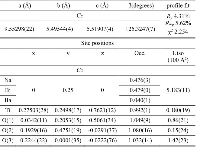
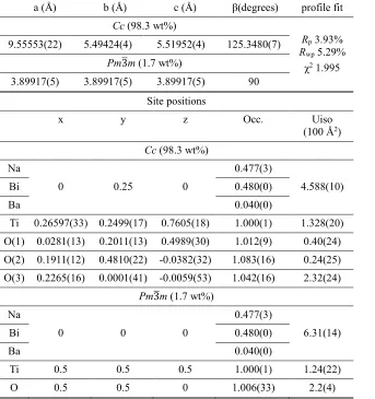
Table 2.1 Data and references for Figure 2.1 ... 19 Table 2.2. Elastic and piezoelectric coefficients used to plot Figure 2.5(a-j). ... 36 Table 5.1. Parameters for the Cc + Pm3̅m phases from the combined Rietveld refinement .. 86 Table 5.2. Parameters for the R3c phase based on the X-ray Rietveld refinement... 86 Table 5.3. Parameters for the Cc phase based on the X-ray Rietveld refinement ... 87 Table 5.4. Parameters for the Cc + Pm3̅m phases based on the X-ray Rietveld refinement .. 88 Table 5.5. Bond valence sum calculations for each bond type in the Cc phase. ... 88 Table 5.6. Structural parameters from the Rietveld refinements of the HRXRD patterns and the neutron PDFs (1-50Å). ... 105 Table 6.1. Parameters for the Rietveld refinement of Na½Bi½TiO3 at 0 kV/mm. The zero-order harmonic, S0(Q) was used for the Rietveld refinement. The atomic displacement
parameters for Ti and O were fixed. ... 133 Table 6.2. Parameters for the Rietveld refinement of Na½Bi½TiO3 at 4 kV/mm. The zero-order harmonic, S0(Q) was used for the Rietveld refinement. The atomic displacement
LIST OF FIGURES
Figure 1.1. An representative polarization vs. electric field (PE) loop. The initial response from an unpoled sample is indicated with a dashed line and arrows indicate the progression of the loop. ... 7 Figure 1.2. Atomic form factors as a function of sin𝜃𝜆 for elements O and Zr. ... 12 Figure 1.3. Pair distribution functions for representative amorphous and crystalline materials. ... 16 Figure 2.1. The general trend between increased piezoelectric properties and increased compliance for different materials and various crystallographic directions. ... 18 Figure 2.2 Schematic of the ToF neutron diffraction instrument VULCAN. ... 22 Figure 2.3. Diffracted intensity and modeled Gaussian peaks for the 111, 200, and 220 peaks of NBT-4BT, NBT-6BT, NBT-7BT, and NBT-13BT. ... 23 Figure 2.4. Lattice strain for selected lattice planes for NBT-xBT. ... 25 Figure 2.5. Elastic anisotropy of NBT-xBT compressed onto the c-a plane. Certain data points are duplicated onto the bottom half of the figure via symmetry. ... 27 Figure 2.6. Elastic (a-e) and piezoelectric (f-j) anisotropies for crystals of various
symmetries and compositions. In the case of the 4mm and mm2 crystals, the vertical direction is the [001] direction, while for the 3m crystals the vertical direction is the [111] pseudocubic direction. See Table 2.2 for the reference data. ... 33 Figure 3.1 Schematic of the WOMBAT instrument noting the scattering vectors of the incident and scattered neutrons and the orientation of the sample electric field vector such that it is aligned with the scattering vector, q, for the diffraction peaks of interest. ... 40 Figure 3.2. (a) Single peak fit for the 111 peak and (b) double peak fit for the 200 peak of NBT-0.13BT showing the measured intensity as solid points and the fit Gaussian curves as a solid line. ... 41 Figure 3.3. Neutron diffraction patterns as a function of electric field for NBT-4BT. The patterns in the main panel are offset for visual clarity. The two smaller panels show the 111 and 200 diffraction peaks. In this case, the 111 peaks exhibits domain switching while the 200 peak exhibits lattice strain. ... 42 Figure 3.4. Neutron diffraction patterns as a function of electric field for NBT-6BT. The patterns in the main panel are offset for visual clarity. The two smaller panels show the 111 and 200 diffraction peaks. In this case, both the 111 and 200 peaks exhibits domain
and 200 diffraction peaks. In this case, the 200 peaks exhibits domain switching while the 111 peak exhibits lattice strain. ... 44 Figure 3.6. Neutron diffraction patterns as a function of electric field for NBT-13BT. The patterns in the main panel are offset for visual clarity. The two smaller panels show the 111 and 200 diffraction peaks. In this case, the 200 peaks exhibits domain switching while the 111 peak exhibits lattice strain. ... 45 Figure 3.7. Lattice strains as a function of electric field for NBT-4BT, NBT-6BT, NBT-9BT, and NBT-13BT. Each panel uses the same scale. ... 47 Figure 3.8. Degree of domain switching as a function of electric field for 4BT, NBT-6BT, NBT-9BT and NBT-13BT. Each panel uses the same scale. ... 49 Figure 4.1. Three cosine functions with difference frequencies in time space. ... 54 Figure 4.2. Three cosine functions transformed to frequency space by the fast Fourier
Transform in MATLAB. ... 55 Figure 4.3. Functions 4 through 6 in the time domain. ... 56 Figure 4.4. Functions 4 through 6 transformed to frequency space by the Fast Fourier
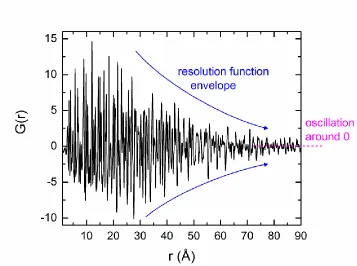
Transform in MATLAB. ... 57 Figure 4.5. Representative G(r) of BaTiO3 with several features highlighted: peak position (purple tick marks); peak area (blue fill); peak height (green lines); and peak width (red lines). ... 60 Figure 4.6. Partial PDFs for the X-ray PDF of BaTiO3. ... 60 Figure 4.7. Experimental X-ray G(r) for BaTiO3 with a representative baseline of -4πρ0r shown in red. ... 62 Figure 4.8. Experimental X-ray PDF of BaTiO3 showing the resolution envelope and that
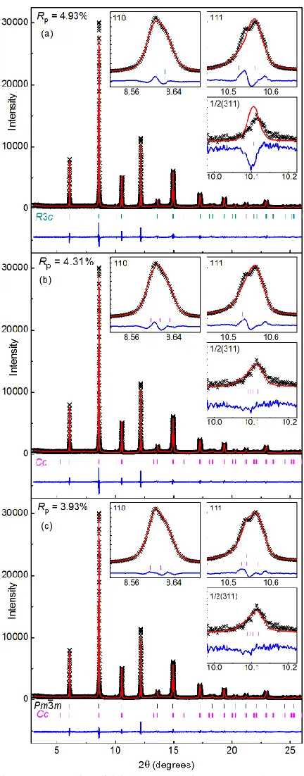
G(r) oscillates around 0 at high r. ... 63 Figure 5.1. Fit of high resolution XRD data to the modeled pattern in a Rietveld refinement of NBT-4BT modeled in the (a) R3c space group, (b) Cc space group, and (c) Cc + Pm3m
line) model are shown, along with the difference pattern and hkl markers below. The insets show magnified views of selected characteristic reflections. ... 98 Figure 5.5. Experimental (red x’s) diffraction pattern and refined (continuous line) model of 0.90BT-0.10BZT using (a) Pm3m space group, and (b) P4mm space group. The difference pattern and hkl markers are shown below. The insets show magnified views of selected characteristic reflections. ... 99 Figure 5.6. Combined X-ray (top panel) and neutron (bottom panel) Rietveld refinement of of 0.90BT-0.10BZT using the P4mm space group. Data (red x’s) and refined (continuous line) model are shown, along with the difference pattern and hkl markers below. The insets show magnified views of selected characteristic reflections. ... 100 Figure 5.7. Experimental (red x’s) diffraction pattern and refined (continuous line) model of 0.92BT-0.08BZT using a two-phase mixture of P4mm and Pm3m space groups. The
difference pattern and hkl markers are shown below. The insets show magnified views of selected characteristic reflections. ... 102 Figure 5.8. Combined X-ray (top panel) and neutron (bottom panel) Rietveld refinement of of 0.92BT-0.06BZT using a combination of P4mm and Pm3m space groups. Data (red x’s) and refined (continuous line) model are shown, along with the difference pattern and hkl
markers below. The insets show magnified views of selected characteristic reflections. .... 102 Figure 5.9. Experimental (red x’s) diffraction pattern and refined (continuous line) model of 0.94BT-0.06BZT using a two-phase mixture of P4mm and Pm3m space groups. The
difference pattern and hkl markers are shown below. The insets show magnified views of selected characteristic reflections. ... 103 Figure 5.10. Combined X-ray (top panel) and neutron (bottom panel) Rietveld refinement of of 0.94BT-0.06BZT using a combination of P4mm and Pm3m space groups. Data (red x’s) and refined (continuous line) model are shown, along with the difference pattern and hkl
markers below. The insets show magnified views of selected characteristic reflections. .... 103 Figure 5.11. The PDF refinement in the range 1-50 Å of 0.80BT-0.20BZT using (a) The
Figure 5.13 The box-car analysis of the PDFs resulted in the lattice parameters shown as red and black symbols. The blue lines indicate the tetragonal lattice parameters obtained from the Rietveld refinements and the dashed pink line represents the lattice parameter for the cubic phase obtained from the Rietveld refinements. Error bars are smaller than the symbols. .... 113 Figure 6.1. Schematic of the measurement setup used to collect the X-ray diffraction (XRD) data under electric field. The sample is rotated toward the incident beam in order to minimize the angle η between the electric field E and the scattering vector Q, for the Q||Esector of the detector. The angular sectors of ±10° used to extract the XRD traces parallel and
perpendicular to the field are indicated using white lines. The sample stage is shown in the inset. ... 121 Figure 6.2. Electric-field-dependent PDFs and residual R.G||(r) for a) BaTiO3, c)
Na½Bi½TiO3,and e) SrTiO3 and the r-dependence of the residual R (equation (2)) for b) BaTiO3, d) Na½Bi½TiO3, and f) SrTiO3. Note that R for BaTiO3 increases approximately linearly with both r and electric field while R for Na½Bi½TiO3 exhibits a distinct jump at 3.25 kV/mm, reaching a much larger maximum value. ... 125 Figure 6.3. Electric-field-dependent G||(r) (top panel) and R (bottom panel) for NBT-4BT.128 Figure 6.4. Electric-field-dependent G||(r) (top panel) and R (bottom panel) for NBT-6BT.128 Figure 6.5. Electric-field-dependent G||(r) (top panel) and R (bottom panel) for NBT-7BT.129 Figure 6.6. Electric-field-dependent G||(r) (top panel) and R (bottom panel) for NBT-9BT.129 Figure 6.7. Electric-field-dependent G||(r) (top panel) and R (bottom panel) for NBT-13BT. ... 130 Figure 6.8. Electric-field-dependent G||(r) (top panel) and R (bottom panel) for HfO2. ... 131 Figure 6.9. Zero-order spherical harmonic of the normalized total scattering. Isotropic S0(Q) for Na½Bi½TiO3 at E=0, 2.75, and 4 kV/mm. ... 132 Figure 6.10. Diffraction data and PDFs of Na½Bi½TiO3. Data are shown for select diffraction peaks (a-b) and G(r) peaks (c-d) as a function of electric field from 0 to 4.5 kV/mm.
Diffraction peaks with scattering vectors aligned with the electric field (a) tend to shift towards lower Q (higher d-spacing) with increased electric field amplitude while diffraction peaks with scattering vectors aligned perpendicular to the electric field (b) tend to shift to higher Q (smaller d-spacing). Select G(r) peaks are shown for both parallel (c) and perpendicular (d) to the electric field. Note that the peak at ≈5.5 Å (pseudocubic cell face diagonal) does not shift. At higher r, peaks in G||(r) tend to shift to higher r while those in
Bi-Bi/Ti-Ti peak corresponding to the distances along the 100PC direction remain relatively unaffected by the field. (b)-(d) Fits (dashed lines) of the experimental 𝐺 ∗ 𝑟 = 𝐺𝑟 + 4𝜋𝑟𝜌0𝑟
(open circles) for 0 kV/mm (b) and 4 kV/mm (QE (c) and Q||E (d)) using the three Bi-Ti distances (R1, R2, and R3), and a single Bi-Bi/Ti-Ti distance. The solid black line in (b)-(d) represents the total fitted profile. ... 139 Figure 6.12. A schematic illustration explaining changes in the directional distributions of the local Bi-Ti distances in Na½Bi½TiO3 under electric field. (a) The change from an unpoled polydomain (only two domains are shown) to a poled monodomain state in the rhombohedral crystal under electric field, E. The polarization vectors in the individual domains are labelled as P. The field is applied along the vertical direction, which coincides with the polar axis of Domain 2. (b) Rendering of a rhombohedral Na½Bi½TiO3 structure in Domains 1 and 2. Only Bi (purple sphere, central) and Ti (blue spheres at cube vertices) atoms are shown. Bi atoms are displaced along the polar axis generating 1 short (R1, red) and 1 long (R3, blue) Bi-Ti distance along that direction. The intermediate distances, labelled as R2 (gray), are formed along all other cube-diagonal directions. For a polydomain crystal, a PDF along either vertical or horizontal (approximately) directions will feature R1, R2, and R3 distances. In contrast, for the poled monodomain state, a PDF along the vertical direction will include only the R1 and R3 distances, whereas a PDF along the horizontal direction will contain only R2. ... 140 Figure 7.1. The 6 default banks in NOMAD in their actual physical locations and pixel positions. The average scattering angle for each bank is noted. The incident neutron beam is shown by the dark red arrow and the sample is at (0,0,0). ... 145 Figure 7.2. I(Q) for the 6 default banks for NOMAD, demonstrating the various Q-ranges and Q-resolutions for each bank. ... 145 Figure 7.3. The detector pixels in NOMAD are divided up into orientation bins that are separated by 15°, as indicated by the different colors. Bin 0 (red) measured scattering parallel to the electric field vector (black arrow) and bin 5 (green) measures scattering perpendicular to the electric field vector. The incident neutron beam is shown by the dark red arrow and the sample is at (0,0,0). ... 146 Figure 7.4. S(Q) for the different orientation bins for a poled sample of NBT. ... 147 Figure 7.5. G(r) for the different orientation bins for a poled sample of NBT. ... 148 Figure 7.6. G(r) for poled and unpoled NBT for the 6 different orientation bins. Bin 0
measures scattering parallel to the electric field vector and Bin 5 measured scattering
values as a function of r; each data point corresponds to a boxed summation range and is plotted at the center of the range. ... 154 Figure 8.2. High- and low-r regions (first two columns) of the PDFs and the R curves (third column) for the model BaTiO3 structures with six different effects applied: thermal
9.2.9. 0.80BaTiO3 – 0.20Bi(Zn1/2Ti1/2)O3 ... 175 Figure 9.10 SEM micrographs of 80BT-20BZT. Grain size measurements were performed on the large image. The others are presented to demonstrate consistency across the sample. .. 175 Figure 9.11 SEM micrographs of 90BT-10BZT. Grain size measurements were performed on the large image. The others are presented to demonstrate consistency across the sample. .. 176 Figure 9.12 SEM micrographs of 92BT-8BZT. Grain size measurements were performed on the large image. The others are presented to demonstrate consistency across the sample. .. 177 Figure 9.13 SEM micrographs of 94BT-6BZT. Grain size measurements were performed on the large image. The others are presented to demonstrate consistency across the sample. .. 178 Figure 9.14. Longitudinal piezoelectric coefficient d33 for different compositions as measured with a Berlincourt d33 meter. ... 180 Figure 9.15. Polarization vs. electric field loops for the studied NBT-xBT compositions. .. 180 Figure 9.16. Polarization vs. electric field loops for the studied BT-xBZT compositions. Reprinted with permission from Ref. 130. Similar PE loops have also been published in Ref. 133... 181 Figure A1. The distribution of angles between Q and E. This distribution of angles is
between the scattering vector (Q) and the electric field (E) in the plane of the detector for a sample that is (a) un-tilted and (b) tilted. ... 207 Figure A2. A representation distribution of Q on the 2D detector for beamline 11-ID-B at the Advanced Photon Source at Argonne National Laboratory for X-rays of energy 58 keV. .. 207 Figure A3. Comparison of PDFs generated using different methods. The G(r) generated via the sine Fourier transform and the ρ(r) via the spherical harmonics approaches for
LIST OF SYMBOLS AND ABBREVIATIONS
PZT Lead zirconate titanate (Pb(ZrxTi1-x)O3) NBT Sodium bismuth titanate (Na1/2Bi1/2TiO3)
BT Barium titanate (BaTiO3)
NBT-xBT Solid solution between NBT and BT
BZT Bismuth zinc titanate (Bi(Zn1/2Ti1/2)O3
BT-xBZT Solid solution between BT and BZT
MPB Morphotropic phase boundary
Di Dielectric displacement
Ei Electric field
σjk Stress (tensor form)
εjk Strain (tensor form)
dijk Piezoelectric coefficient (tensor form)
dij Piezoelectric coefficient (matrix notation)
Pr Remnant polarization
Ec Coercive field
εr Dielectric constant or relative permittivity
ε0 Permittivity of free space
χij Susceptibility (matrix notation)
Sij Elastic compliance (matrix notation)
P Polarization
XRD X-ray diffraction
ND Neutron diffraction
SEM Scanning electron microscope
TEM Transmission electron microscope
λ wavelength
ToF Time-of-flight
εhkl Lattice strain
Ihkl Integrated intensity of the hkl diffraction peak
ηhkl Degree of domain switching
Rp R-pattern for Rietveld refinements
Rwp R-weighted-pattern for Rietveld refinements
χ2 Chi squared goodness-of-fit parameter
U Atomic displacement parameter
d Spacing between lattice planes
Q Scattering vector
I(Q) Intensity as a function of Q
S(Q) Total scattering function
PDF Pair distribution function
G(r) Reduced pair distribution function
G*(r) or R(r) Radial distribution function
R r-dependent normalized difference between PDFs
η Angle between Q and E
CHAPTER 1
INTRODUCTION AND BACKGROUND
1.1 Introduction
Ferroelectric and dielectric ceramics are used in a multitude of applications including sonar, ultrasound, micro-positioning, actuators, and transducers, capacitors, and ferroelectric
memories.1-3 Commercially leading compositions are mainly lead(Pb)-based; the solid solution of PbZrO3 and PbTiO3, Pb(ZrxTi1-x)O3 (PZT), has found many uses and is currently
the most popular material, partly due the ease with which its properties can be modified.1,4 Single crystals of Pb(Mg1/3Nb2/3)O3-PbTiO3 and Pb(Zn1/3Nb2/3)O3–PbTiO3 are used in
actuator applications because of their exceptionally large piezoelectric response.,5-7 However,
due to the toxicity of lead to humans and its negative environmental impact, legislation in the European Union seeks to remove lead from consumer products.8 A universal lead(Pb)-free
replacement to PZT has not yet been found, although there are various lead-free
compositions that show promise for replacing PZT in certain applications.8,9 Many are based on the classical ferroelectric BaTiO3 (BT) while others are based on Na1/2Bi1/2TiO3 (NBT),
which exhibits relaxor ferroelectric features (see sections 1.1.1 and 1.1.2).8 In particular, KNbO3-based materials show promise for high-frequency transducers, such as those used in
skin-imaging applications.9 Materials based on the solid solution between NBT and BT (NBT-xBT) have high mechanical quality factors and can be used in high vibration velocity and high power applications.9 Such materials are being commercially manufactured for
1.1.1 BaTiO3
BaTiO3 and its ferroelectric properties were discovered simultaneously in several
parts of the world between 1941 and 1946.4 When the dielectric constant was measured, it was found to be 1100, significantly higher than the best-known at the time, 100 for the rutile phase of TiO2.4 The understanding that piezoelectricity could be evoked from a ceramic was
realized around 1946, and was dependent on the discovery of the process of poling. Since then, development has been rapid and BaTiO3-based ceramics remain popular and useful.
At synthesis temperatures (~1400°C) down to 130°C, BaTiO3 exists as the cubic
aristotype structure with 𝑃𝑚3̅𝑚 symmetry. Below this temperature, it transitions to a tetragonal phase where the c-axis is slightly elongated, as described by the P4mm space group, and the long-range polarization direction is along [001]. At 0°C, BaTiO3 transitions to an orthorhombic structure with space group Amm2, where the long-range polarization
direction is along [011]. Finally at -90°C, BaTiO3 takes on a rhombohedral structure with space group R3m and the long-range polarization direction is along [111].11 There is,
however, controversy regarding the local displacements in BaTiO3 across the different phase transitions. It has been found via X-ray and neutron total scattering that the Ti4+
displacements are always along the [111] direction, regardless of the temperature.12-14
Instead, it is thought that for the different phases, Ti4+ occupies different proportions of the eight possible [111] displacement variants (towards each of the 8 faces of the TiO6
phase, two of the eight sites are populated (averaging out to a {101} direction; and in the rhombohedral phase, only one of the eight sites would be occupied, corresponding to
observed long range [111] polarization direction.
Property-wise, BaTiO3 ceramics attain a longitudinal piezoelectric coefficient, d33, of between 191 and 250 pC/N and relative permittivities of over 5000, both of which are
dependent on grain size.15,16 At room temperature, the coercive field is around 0.3 kV/mm and the remnant polarization is around 8 μC/cm.4 The spontaneous single crystal polarization
is around 26 μC/cm.4
1.1.2 Na1/2Bi1/2TiO3
Sodium bismuth titanate, Na1/2Bi1/2TiO3, or NBT, was originally discovered in 1960 by Smolenskii et al. and was observed to have a cubic perovskite structure.17 Modern studies
have shown the structure to be far more complicated. In 2002, Jones and Thomas identified the temperature-dependent phases of Na1/2Bi1/2TiO3 to be a high temperature cubic phase above 540°C, a tetragonal phase with space group P4bm from 400-500°C, and a
rhombohedral phase with space group R3c from 255°C to -268°C.18 Later, from the same group, using single crystals of NBT, Gorfman and Thomas evidenced a “non-rhombohedral
average structure,” which they identified as the monoclinic Cc space group.19This structure
was confirmed through high-resolution X-ray diffraction (HRXRD) measurements on ceramics of NBT by Aksel et al.20 In a later work, Aksel et al. found that adding a small
pattern.21 Even more recently, the coexistence of both Cc and R3c ferroelectric phases in pure, unpoled NBT has been evidenced.22
Studies which utilize local structure probes such as PDFs and/or transmission electron microscopy (TEM) have evidenced additional structural complexities. Studies by both
Keeble et al. and Aksel et al. have found that the Bi3+ coordination environment differs from
the Na+ environment and that the Bi-O bonds exhibit a bimodal distribution.23,24 Through careful analysis and modeling, Keeble et al. showed that Bi3+ is preferentially displaced from
the centroid of its oxygen polyhedral, and at room temperature, this displacement is centered along the monoclinic plane near, but not exactly towards, the rhombohedral polarization direction.24 In a TEM study, Levin and Reaney proposed that NBT consists of nanodomains
of a-a-c+ tilting, where the in phase tilting (c+) (i.e., a tetragonal structure) is coherent over only a few unit cells.25 Prior studies also utilizing TEM also identified tetragonal platelets
within a rhombohedral matrix.26,27 Additionally, Levin and Reaney found that the Bi3+ and Ti4+ cations exhibit polar displacements.25 According to this model, domain averaging over
longer length scales would result in an average 𝑎−𝑎−𝑐−- tilt structure, which concurs with the
HRXRD studies mentioned above.
Despite the structural complexities, NBT is a component in many lead(Pb)-free compositions of research interest and compositionally-modified NBT has shown promise for
1.2 Fundamentals
1.2.1 Piezoelectricity and Ferroelectricity
Piezoelectricity was first discovered in 1880 by J. and P. Curie when they found that certain crystals exhibit an electric charge when a mechanical stress is applied to them.4 The
converse effect also occurs such that the crystal will strain when an electric field is applied. Both effects are linear. For a crystal to be able to exhibit piezoelectricity, its atomic structure
must be not have a center of inversion.
Dielectric displacement, Di (Di = Q / A, where Q is charge and A is area), is related to the stress applied σjk, by the piezoelectric coefficient dijk, and this is referred to as the direct
effect (Equation 1-1). The converse effect occurs when a strain εjk is caused by an applied electric field Ei (Equation 1-2). The piezoelectric coefficient is a third rank tensor as it relates
a first rank tensor (dielectric displacement Di or electric field Ei) and a second rank tensor
(stress σjk or strain εjk). In full tensor notation, the relation is
𝐷𝑖 = 𝑑𝑖𝑗𝑘𝜎𝑗𝑘 (1-1)
for the direct effect and
𝜀𝑗𝑘 = 𝑑𝑖𝑗𝑘𝐸𝑖 (1-2)
for the converse effect. dijk is numerically equivalent for either case.
Typically, the “matrix notation” is used, which reduces the number of independent piezoelectric coefficients, which results in the two following relationships.
𝜀𝑗 = 𝑑𝑖𝑗𝐸𝑖 (1-4)
where i, j = 1, 2, 3, 4, 5, or 6.
The units for dij are either coulombs/Newton or meters/volt (typically reduced to
pC/N or pm/V) and are numerically equivalent. In practice, one is usually interested in the piezoelectric response in the same direction as the applied stimulus, which is described for
both the direct and converse effects as d33. Also of interest is the piezoelectric response in the
transverse direction (noted as 1), which is the d31coefficient.
Ferroelectrics are piezoelectrics that exhibit a spontaneous polarization at the unit cell
level even in the absence of an applied electric field and this spontaneous polarization can be reoriented by an applied electric field.4 However, due to the method by which polycrystalline
ferroelectrics are synthesized (often a two-step solid-state process consisting of a calcination (i.e., reaction) step following by a sintering (i.e., densification) step), the macroscale sample lacks net polarization in the as-processed state. The individual grains have many different
orientations and each grain is typically divided into contiguous areas where the spontaneous polarization is oriented in the same direction. The division into smaller areas with different
polarization directions occurs to compensate the charge build-up. These areas are referred to as domains and are separated by domain walls. While each domain exhibits a spontaneous
polarization, overall, the ceramic is isotropic because the different domain and grain
orientations result in a net polarization of zero. The direction of the spontaneous polarization can be reoriented with a sufficiently strong electric field, i.e., one of greater amplitude than
macroscale polarization is called poling.4 The process by which the polarization direction of each domain changes orientation is called domain switching or domain reorientation.30 The
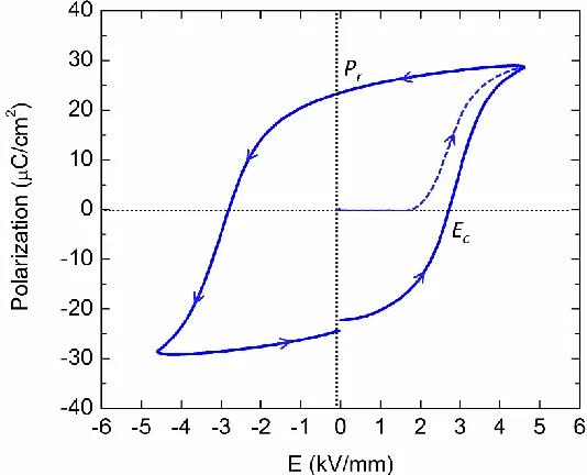
coercive field, Ec, can be determined by measuring polarization as a function of applied electric field during a bipolar electric field cycle (e.g. 0 5 0 -5 0 kV/mm), as
shown in Figure 1.1. This method also determines the remnant polarization, Pr , the
polarization which remains at zero field after the maximum field is achieved. The hysteresis present in PE loops is a key characteristic for ferroelectrics.
Figure 1.1. An representative polarization vs. electric field (PE) loop. The initial response from an unpoled sample is indicated with a dashed line and arrows indicate the progression of the loop.
The phenomenon of ferroelectricity was first discovered in Rochelle Salt in 1921 by
materials. Therefore, the name “ferroelectric” does not refer to any iron (Fe) content in
ferroelectric materials, but rather their analogous behavior to ferromagnets.
1.2.2 Polarization and dielectric permittivity
There are four mechanisms which can contribute to the macroscopic polarization of a
material. They are atomic, ionic, dipolar, and space charge, in order of smallest to largest length-scale.32,33 The strengths of the different mechanisms are quantified by their dielectric
constant, which is a measure of how much electric charge can be stored by a material, e.g., if used as a parallel plate capacitor. These four mechanisms can contribute additively to the total dielectric constant. The ability to store charge is quantified by
𝐷 = ε𝐸 (1-5)
where D and E are the same dielectric displacement and electric field from Equation 1-1, and
ε is the electric permittivity.33 The dielectric constant or relative permittivity ε
r is normalized by the permittivity of free space, ε0 = 8.85 ∙ 10-12 F/m, by
ε𝑟 = ε/𝜀0 (1-6)
The electronic mechanism arises from the displacement of an atom’s electron cloud
relative to the nucleus. This is the only possible polarization mechanism for covalent materials such as diamond.33 The contribution to the dielectric constant for this effect is
Ionic polarization occurs when positive and negative ions displace slightly in opposite directions when in the presence of an electric field and occurs in all ionic materials. The
magnitude of ionic polarization P can be determined from
𝑃 = 𝑞 × 𝑑 × 𝑁 = 𝜀0(𝜀𝑟− 1)𝐸 (1-7)
in which the total charge of the positive or negative ions is q, the displacement is d, the
density of dipoles is N, which is also 1/(unit cell volume), the permittivity of free space is ε0, the relative permittivity is εr, and the electric field is E. In this case, εr should be the portion of the permittivity arising from the ionic polarization mechanism. For ionic materials such as
NaCl, the ionic polarization contribution to the dielectric constant increases it to 6-10.33 Dipolar polarization is the reorientation of dipoles within a material due to an electric
field. This occurs within a ferroelectric when it undergoes the poling process via the process of domain reorientation discussed in 1.2.1, and will be quantified in Chapter 3. The
contribution of this mechanism to the dielectric constant is orders of magnitude larger and
results in dielectric constants of several 1000 for oxide ferroelectrics like PZT and BT.4,33 The space charge mechanism is also called interfacial or diffusional polarization and
occurs when mobile charges drift under the influence of an electric field and are pinned at interfaces or boundaries within a material. This mechanism results in the highest measured dielectric constants. For example, in dense ceramics of composition Ba0.95La0.05TiO3–x with a
1.2.3 Scattering and diffraction of X-rays and neutrons
To determine the structure of a material at the atomic level, the experimental
technique of diffraction is widely used. In the general sense, diffraction is the coherent and elastic scattering of radiation of appropriate energy from a collection of atoms. Materials scientists are primarily interested in the pattern of constructive interference that occurs after
the radiation interacts with a material. This diffraction pattern can reveal the structure of a material. Materials science is primarily concerned with diffraction of X-rays, neutrons, and
electrons, though this work only covers X-ray and neutron diffraction.
X-rays are electromagnetic radiation. Like all electromagnetic radiation, a beam of such radiation can be thought of as a wave or as a stream of photons which travel at the speed
of light, c (or more precisely, the speed of light through air or the medium within a given instrument). By definition, X-rays have wavelengths between 0.01 and 1.0 nm.35 When a
beam of coherent X-rays is directed at a material, they interact with atoms/ions primarily through absorption or scattering off of the electron cloud of an atom or ion. The scattering from a collection of atoms results in diffraction.
Neutrons of appropriate energy can also undergo diffraction when such a beam is incident on a material (thanks to wave-particle duality). Neutrons do not travel at the speed of
light; their energy is proportional to their velocity and can be adjusted by passing them through moderators of different temperatures after their birth in a reactor or spallation source. ‘Thermal’ neutrons are passed through moderators at approximately room temperature,
range of wavelengths for X-rays).36 Neutrons scatter from an atom or ion’s nucleus, not the electron cloud, which gives neutron diffraction unique properties compared to X-ray
diffraction.37
This brief introduction to diffraction begins with the scattering of X-rays from a single electron, then continues onto scattering from a single atom, and finally scattering from
a unit cell of atoms, at which point we can pick back up with neutron scattering. Scattering of X-rays from a single electron can be computed from the Thomson
equation, which calculates the intensity I as a function of the incident intensity I0 and angle α, which is the angle between the scattered X-rays and the direction in which the electron is accelerated (parallel to the electric field component of the X-ray radiation).35K is a very
small constant ~10-30 m2.
𝐼 = 𝐼0
𝐾
𝑟2sin2𝛼
(1-8)
After considering the components along the perpendicular directions and combining them, the total scattered intensity at a point away from the electron is35
𝐼 = 𝐼0 𝐾 𝑟2(
1 + cos2𝜃
2 ) (1-9)
For relevant diffraction geometries, r is very large compared to an atom, and the K/r2
term can be safely ignored. The angle-dependent term is referred to as the polarization factor. The intensity of coherently scattered X-rays from a single atom depends on which element the atom is and also on the angle at which the intensity is measured from the incident
𝑓(𝑠) = 𝑍 − 41.782 × 𝑠2× ∑ 𝑎𝑖𝑒−𝑏𝑖𝑠2
𝑁
𝑖=1
(1-10)
where s = sin 𝜃 𝜆⁄ in Å-1, θ is the angle, λ is the wavelength of the X-rays, and ai and bi are
element-specific terms, of which there are three or four per element.35 Figure 1.2 shows representative form factors for O and Zr. Note that in the forward scattering direction, i.e.,
θ=0, the scattered intensity, f, is equal to the atomic number for O (8) and Zr (40). The form
factor, f (s), controls the angular dependence of the decreasing scattered intensity that occurs for X-ray diffraction patterns. (The scattering factor is also briefly covered in 4.3.1. in the
context of the corrections applied to X-ray total scattering data detected using a 2D detector.) There is no angle-dependent form factor for neutrons because neutrons scatter from atomic nuclei and not the electron cloud. The nucleus can be considered as a true point
scatterer, so the scattering factor is constant as a function of angle and would appear as a flat line on Figure 1.2.35
For a crystalline solid undergoing diffraction, intensity as a function of scattering angle is related to the crystal structure through the structure factor Fhkl,
𝐹ℎ𝑘𝑙 = ∑ 𝑓𝑛(𝑠)𝑒2𝜋𝑖(ℎ𝑥𝑛+𝑘𝑦𝑛+𝑙𝑧𝑛)
𝑁
𝑛=1
(1-11)
where for atom n, fn(s)is the scattering factor (which is a factor of s), hkl are the Miller
indices of the hkl plane undergoing diffraction, and xyz are the fractional coordinates of the atom within the unit cell scattering the X-rays.35
Similarly, for neutrons,
𝐹ℎ𝑘𝑙 = ∑ 𝑏𝑛𝑒2𝜋𝑖(ℎ𝑥𝑛+𝑘𝑦𝑛+𝑙𝑧𝑛)
𝑁
𝑛=1 (1-12)
where bn is the coherent scattering length for neutrons for each atom type.36
What we actually measure with a detector though is just the intensity of the diffracted
X-rays or neutrons, Ihkl = |Fhkl |2. Because we can only measure the intensity, the phase
information, i.e., the relative phase difference from the diffracted X-rays is lost.
More simple and fundamental than the structural factor is Bragg’s law, which describes conditions at which diffraction occurs. For a monochromatic beam of X-rays incident on a crystalline material, the X-rays “reflect” off lattice planes. The reflected X-rays
may interfere constructively or destructively at different reflection angles. Bragg’s law identifies conditions at which constructive interference occurs, and is written as,
where λ is the wavelength of the radiation, d is lattice spacing of the planes undergoing diffraction, and θ is the half the scattering angle, 2θ.38 It states that for a given lattice spacing
and wavelength, there is an angle such that constructive interference occurs and a maxima in intensity is observed. Derivations can be found in many books35, including those introducing materials science to undergraduate students for the first time.32
1.2.3.1 Rietveld refinement
Rietveld refinement is a crystallographic structure refinement method which refines a crystal structure against an experimental powder diffraction pattern. The method was first published by Dr. Hugo Rietveld in 1967, and further in 1969.39,40 The method refines a
starting crystal structure by calculating the diffraction pattern from the given structure, modifying it based instrumental parameters, peak shape functions, background subtraction,
and other effects, and comparing it to the experimental diffraction pattern. The difference between the calculated and experimental patterns is minimized with a least-squares
regression algorithm. The required starting information is the space group, atomic positions,
occupancies, and atomic displacement parameters, background subtraction, instrumental information including the wavelength or time-of-flight (ToF) constants for ToF neutron data,
peak shape functions, and if desired, preferred orientation functions. Generally, most of the parameters except the instrumental ones are refined until the refinement converges to a satisfactory solution. There many different Rietveld software packages including FullProf,
refinement and lies at the forefront of crystallography, having received thousands of citations over the years, and continues to be advanced as evidenced by the recent release of
GSAS-II.43,44
1.2.3.2 Pair distribution functions
Rietveld refinement and other crystallographic methods are powerful and useful, however, they typically fall short in analyzing the structures of liquids and amorphous
materials because diffraction of these types of materials do not result in sharp Bragg diffraction peaks. Fortunately, there is an alternate approach, called total scattering, which utilizes the information present in both the sharp Bragg peaks and the diffuse scattering,
which contains information about defects and disorder in a material. By applying a Fourier transform to a total scattering pattern, a pair distribution function (PDF) can be calculated.
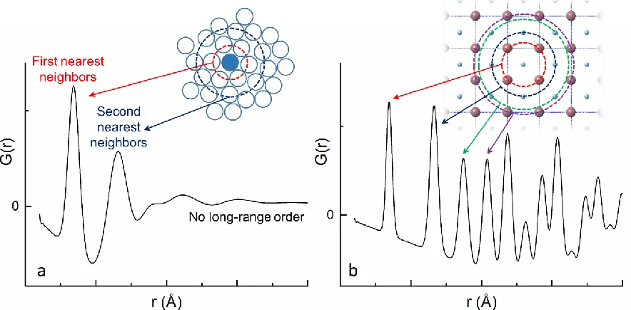
This method reveals the structure of a material in real-space, as opposed to reciprocal space, as in diffraction. A PDF is the probability of the existence of atom-atom pairs as a function of distance for all atoms in a sample, as shown in Figure 1.3. for representative
amorphous/liquid and crystalline materials. PDF studies have been found to be a useful tool to characterize the structural complexity of functional materials, such as ferroelectric
Figure 1.3. Pair distribution functions for representative amorphous and crystalline materials.
1.3 Dissertation Outline
Chapters 2 and 3 describe the response of the lead-free ferroelectric NBT-xBT to uniaxial stresses and electric fields, respectively, using in situ neutron diffraction. Chapter 4
provides background information on pair distribution functions. Chapter 5 includes both X-ray diffraction and neutron pair distribution function studies performed at ambient
conditions. Chapters 6 describes results from the novel methodology of measuring X-ray
total scattering during in situ application of electric fields. Chapter 7 shows preliminary ex situ results from neutron PDF experiments on poled and unpoled Na1/2Bi1/2TiO3 ceramics.
CHAPTER 2
IN SITU NEUTRON DIFFRACTION EXPERIMENTS I: MECHANICAL STRESS
2.1 Motivation
Ferroelectric ceramics are used in both sensors and actuators due to their ability to interconvert mechanical and electrical energy.5 While the electrical properties of ferroelectric materials are most often studied, an understanding of the elastic properties and response to
applied mechanical loads is also of fundamental importance.45 Elastic properties have been identified as crucial for the performance of actuators, as they affect the magnitude of the
piezoelectric response, with elastic softness typically corresponding to a large piezoelectric response.46,47 For instance, the large elastic compliance of the rhombohedral phase of
PbZn1/3Nb2/3O3–PbTiO3 (PZN–PT) has been suggested as the mechanism for the so-called “giant” piezoelectric effect found in this material.48,49
Elastic (and other electromechanical) constants of ferroelectric crystals can be
determined using the resonance technique, which measures impedance as a function of frequency.50,51 Additionally, elastic stiffnesses or compliances and piezoelectric coefficients
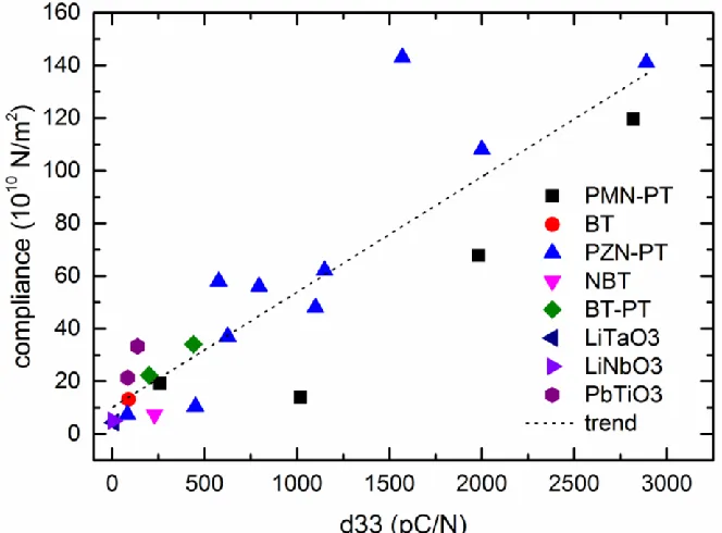
of single crystals can be measured by the ultrasonic pulse-echo technique, which utilizes the fact that the speed at which an elastic wave moves through the material depends on the material’s elastic constants.50,52 Figure 2.1 presents macroscopic compliance and d
33 data for a variety of single crystal materials, where there is an observable tendency toward increased compliance (i.e., elastic softness) and an increased piezoelectric response. Table 2.1 lists the
synthesized as single crystals in order to perform such measurements, such as the
commercially useful lead zirconate titanate (Pb(ZrxTi1-x)O3 or PZT).53 Single-crystal elastic
constants for PZT are not yet reported. In ceramic form, a compositional phase boundary exists near x=0.52 between a Ti-rich tetragonal phase and a Zr-rich rhombohedral phase at which many electromechanical properties are maximized.54,55 It has been observed that for
PZT ceramics, the elastic compliance also peaks at the compositional phase transition between the tetragonal and rhombohedral phases.55 When investigating the mechanical
properties for a given PZT composition as function of temperature, it has been found that the elastic modulus has local minima (equivalent to a maximum in the compliance) at the
temperature-dependent phase transitions in PZT ceramics as well.47
Table 2.1 Data and references for Figure 2.1
Composition d33 (pC/N) Compliance (1010 N/m2) Ref.
PMN 42-PT [001] 260 19.21 56
PMN-29PT [001] 1020 13.9 57
PMN-30PT [001] 1981 67.7 56
PMN-33PT [001] 2820 119.6 56
BaTiO3 SC 90 13.1 58
PZN [111] 83 7.4 6
PZN [001] 1100 48 6
PZN-4.5PT 2000 108 59
PZN-8PT 2890 141 59
PZN-9PT (R) [001] 1570 143 60
PZN-9PT (T) [001] 795 56 60
PZN-9PT (R) [111] 625 36.9 60
PZN-9PT (T) [111] 450 10.3 60
PZN-7PT [110] 1150 62.0233 59
PZN-12PT 576 58 59
Na1/2Bi1/2TiO3 230 7.3 46
BS-64PT 440 34 61
BS-66PT (T) 200 22.32 62
LiTaO3 8 4.36 63
LiNbO3 6 5.02 63
PbTiO3 136.6 33.3 64
PbTiO3 83.7 21.3 65
Despite the widespread commercial use of PZT and other Pb-based ferroelectrics,
there is increasing interest in Pb-free ferroelectric materials due to legislation which seeks to decrease the usage of Pb in consumer products.8 Several recent compositions are based on sodium bismuth titanate (Na0.5Bi0.5TiO3, or NBT) and/or BaTiO3 (BT), both of which adopt
the ABO3 perovskite structure. Given the importance of elastic properties to the performance of ferroelectrics, this work investigates the elastic response to uniaxial stresses of four
system by investigating the elastic and piezoelectric anisotropies for various compositions/symmetries.
2.2 Experimental
2.2.1 Sample synthesis
Polycrystalline samples of NBT-4BT, NBT-6BT, NBT-7BT, and NBT-13BT were
selected for this study based on their positions across the NBT-xBT phase diagram. NBT-4BT lies between pure Na1/2Bi1/2TiO3 and the morphotropic phase boundary (MPB) region,
which has been identified located at ~7% BT or in the range 6-10% BT.66,67 Compositions NBT-6BT and NBT-7BT were selected because they are in the MPB region, and NBT-13BT
because it lies on the tetragonal side of the MPB region. The solid solution of Na1/2Bi1/2TiO3
-xBaTiO3 is discussed more fully in section 5.2.1. The samples were synthesized from stoichiometric ratios of reagent grade powders of Na2CO3 (99.5% purity), TiO2 (99.6%
purity), Bi2O3 (99.975% purity), and BaTiO3 (99.7% purity, all Alfa Aesar) through a solid oxide processing route. Reactant powders were ball-milled in ethanol for 24 h with 5 mm
yttria-stabilized zirconia milling media using a ball to powder ratio of 10:1. The powders were dried at 100 °C, ground with a mortar and pestle, and passed through a 200 μm sieve.
The powders were calcined at 900°C for 4 h in covered alumina crucibles with heating and
cooling rates of 5 °C/min. Approximately 30 g of powder was uniaxially pressed in a 25 mm square hardened steel die at 2 metric tons for 5 min to form a pellet, followed by isostatic
heating and cooling rates of 5 °C/min. Rectangular prisms were cut from the sintered pellets with a diamond saw. Samples were prepared for loading by machining parallel sides to
prevent stress concentrations during compression. Typical sample dimensions were ~10 mm x ~10 mm x ~20 mm.
2.2.2 In situ neutron diffraction
In situ neutron diffraction patterns were measuredduring static compressive loading,
using a 100,000 N capacity hydraulic load frame, on the instrument VULCAN, a time-of-flight (ToF) diffractometer at the Spallation Neutron Source, Oak Ridge National
Laboratory.68 A schematic of the instrument is shown in Figure 2.2. The samples were
clamped in place by the platens. Stresses were increased in 25 MPa increments until sample failure. Diffraction patterns were measured for approximately 15 min at each stress level with
a detector that recorded diffraction patterns from lattice planes with their normals parallel to the applied stress. As this is a ToF diffractometer, each diffraction pattern is the sum of diffracted neutrons from sets of different crystallographic planes that have the same spatial
orientation; in this case, the normals of all the diffracting planes are parallel to the applied stress. The diffraction patterns were normalized to a vanadium standard background pattern
Figure 2.2 Schematic of the ToF neutron diffraction instrument VULCAN.
2.2.3 Single peak fitting
Single peak fitting was performed on selected Bragg reflections in the normalized patterns using a least squares algorithm with a Gaussian profile shape function in the
program MATLAB (The Mathworks Inc., ver. 7.6.0.324), which provided the peak center positions (dhkl) and peak integrated intensities (Ihkl).
Due to a small degree of splitting in certain twin-related reflections (e.g. the 111/111̅
peak in rhombohedral perovskites), the constituent peak widths were constrained to be equal,
which allowed more reliable peak fitting as the peak intensities increased or decreased with applied load. To further improve the reliability for the fitting of the 200/002 reflection of
Figure 2.3. Diffracted intensity and modeled Gaussian peaks for the 111, 200, and 220 peaks of NBT-4BT, NBT-6BT, NBT-7BT, and NBT-13BT.
Figure 2.3 shows the pseudocubic 111, 200, and 220 reflections in 4BT, NBT-6BT, NBT-7BT, and NBT-13BT at the initial 3 MPa stress and at 200 MPa; 3 MPa was the
the fracture stress of all compositions. The measured intensity is shown as symbols and the Gaussian fits are shown as lines. NBT-4BT exhibits pseudo-rhombohedral symmetry, with a
split 111/111̅ peak. NBT-13BT shows tetragonal symmetry, with a split 200/002 peak. The compositions near the MPB (NBT-6BT and NBT-7BT) do not show observable splitting.
However, the 200 peak in NBT-7BT broadens with increasing stress, possibly due to an unresolved tetragonal distortion, or strain broadening.
2.2.4 Linear fitting of stress-strain curves in the elastic region
Using the parameters from the peak fitting process, lattice strains were determined as
a function of applied stress. The lattice strain, εhkl for selected crystallographic planes with
normals parallel to the applied uniaxial stress were calculated using the fitted peak center positions (dhkl) with Equation 2-1.
𝜀ℎ𝑘𝑙 =
𝑑ℎ𝑘𝑙 𝑖𝑛𝑖𝑡𝑖𝑎𝑙−𝑑ℎ𝑘𝑙 𝑓𝑖𝑛𝑎𝑙
𝑑ℎ𝑘𝑙 𝑖𝑛𝑖𝑡𝑖𝑎𝑙 (2-1)
Figure 2.4 shows the compressive strains as a function of uniaxial compressive stress for selected lattice planes for the four compositions. The stress at which the curves terminate
is the stress at which the samples failed; NBT-6BT failed at a higher stress than the other compositions.
In order to extract further information regarding the elastic properties, linear fits of
the stress-strain curves were performed on the elastic region of the curves. The slope of the linear fit is the elastic modulus for the lattice planes which correspond to the selected
response becomes non-linear. However, this stress value is not the same for all the
compositions. The stress value for the end of the elastic region was determined by comparing
the goodness of fit values for the linear fits of each reflection up to 75, 100, 125, and 150 MPa. The terminal stress was 125 MPa for NBT-4BT, 75 MPa for NBT-6BT and NBT-7BT, and 150 MPa for NBT-13BT.
Figure 2.4. Lattice strain for selected lattice planes for NBT-xBT.
The elastic stiffness Ehkl (i.e., elastic modulus) was determined using the slope of the
𝐸ℎ𝑘𝑙 = 𝜎ℎ𝑘𝑙⁄𝜀ℎ𝑘𝑙 (2-2)
It has been noted previously that Equation 2.2 can be carried out as the full tensor relationship, but in practice, reduction to Hooke’s law is an effective and practical
approximation for uniaxial loading.70 Similarly, lattice strains due to an electric field can be used to determine the electric-field strain coefficient, d.71
To verify the trends obtained from the above method, an additional method of calculating Ehkl was utilized for NBT-6BT. A second order polynomial fit was used to fit the
stress vs. strain data and the coefficient for the linear term was used to determine the elastic
stiffness. The use of this method resulted in slightly different values but similar trends in orientation (hkl)-dependence.
2.3 Elastic Anisotropy
The values obtained for Ehkl for the various sets of planes for each composition are
plotted in Figure 2.5 in the form of a polar plot. The length of the radius (from the center to the points on each of the red, green, black, and blue lines) is the magnitude of the elastic
stiffness Ehkl for the given lattice planes and composition. The angles are those between the
particular crystallographic direction measured and the vertical [001] direction of the crystal (i.e., the tetragonal c-axis is at zero degrees). For example, the (111) plane is located at
Figure 2.5. Elastic anisotropy of NBT-xBT compressed onto the c-a plane. Certain data points are duplicated onto the bottom half of the figure via symmetry.
2.4 Discussion
There are few reports in the literature on the elastic anisotropy of ferroelectric ceramics. However, in reports by Heifets et al. and Cohen et al., the authors simulated the
elastic anisotropies for tetragonal and rhombohedral phases of PZT with a 50/50 Zr/Ti ratio.45,73 These studies provided calculated single crystal elastic constants, which could be