YANG, XINGZHOU. Immersed Interface Method for Elasticity Problems with Interfaces. (Under the direction of Dr. Zhilin Li)
PROBLEMS WITH INTERFACES
by
Xingzhou Yang
a dissertation submitted to the graduate faculty of north carolina state university
in partial fulfillment of the requirements for the degree of
doctor of philosophy
department of mathematics
raleigh
June 17, 2004
approved by:
Chair: Dr. Zhilin Li Dr. Kazufumi Ito
Xingzhou Yang was born in November, 1967 in Xuzhou, Jiangsu Province, the People’s Republic of China. He received his Bachelor of Science degree in Mathematics in 1989 and Master of Science degree in Applied Mathematics in 1997 from Nanjing University. He joined the faculty of Nanjing University as instructor in 1989 and then lecturer from 1991 to 1999. The courses he taught include Calculus of all levels, Linear Algebra, Differential Equations etc. He was ever a leader in the teaching group for “Higher Mathematics for Adults(night school)”. In the academic year 1997-1998, he received an award for excellent teaching.
In the fall of 1999, he entered the Ph. D. program in Applied Mathematics with a concentration in Computational Mathematics at North Carolina State University.
I am very grateful for my advisor, Dr. Zhilin Li, for his guidance, suggestions and encour-agement, and for his contributing to my professional development. I would like to thank Dr. Kazufumi Ito, Dr. Bo Li, Dr. Xiao-biao Lin and Dr. Mansoor A. Haider for their directions and suggestions. I also would like to thank Dr. Harvey Charlton, Dr. Ernie L. Stitzinger, Administrator of graduate program, and the departmental secretaries Ms. Di Bucklad, Ms. Brenda Currin and Ms. Denise Seabrooks for their kind help throughout my Ph. D. study at NCSU.
In addition, I want to thank my parents for their support and love. I thank my friends Taiping He and Lihan Zhang for their generous help. Finally and most importantly I want to thank my wife, Yan Wang, for her love, support and understanding.
This research was partially supported by ARO grants 39676-MA, 43751-MA, NFS grants DMS-0073403 and DMS-0201094.
List of Tables viii
List of Figures ix
1 Introduction 1
1.1 An overview of interface problems . . . 1
1.2 Elasticity problems with interfaces . . . 5
1.3 Outline of the thesis . . . 8
2 IIM using Finite Difference for Elasticity Problems with Interfaces 10 2.1 Description of the Algorithm . . . 11
2.1.1 Classification of grid points . . . 12
2.1.2 Discretization at regular grid points . . . 12
2.1.3 Discretization at type I irregular grid points . . . 14
2.1.4 Discretization at type II irregular grid points . . . 16
2.2 Transformations of Local Coordinates . . . 18
2.3 Interface Relations . . . 18
2.3.2 Interface relations for u+1ξη andu+2ξη . . . 23
2.3.3 Interface relations for u+1ξξ and u+2ξξ . . . 25
2.4 Derivation of the Finite Difference Scheme at Type I Irregular Grid Points . 26 2.5 Numerical Examples . . . 33
2.6 Summary of IIM using the finite difference scheme . . . 39
3 Immersed FEM for Elasticity Problems with Interfaces 42 3.1 Formulation of finite element equations . . . 44
3.1.1 Variational form . . . 45
3.1.2 Another derivation of the weak form . . . 46
3.1.3 Finite element equations . . . 48
3.2 Basis functions . . . 48
3.2.1 Basis functions on non-interface elements . . . 49
3.2.2 Basis functions on interface elements . . . 54
3.3 Assembling the stiffness matrix and the load vector . . . 63
3.4 Gaussian Quadrature . . . 71
3.5 Level set interpolations . . . 74
3.6 Solution of finite element equations . . . 76
3.7 Numerical examples . . . 77
4 Conclusions and future work 84
A.1 Fortran 90 subroutine geometry 3tx . . . 87
A.2 Fortran 90 module irreg mod . . . 89
A.3 Fortran 90 subroutine coeff . . . 98
List of References 103
2.1 The grid refinement analysis for Example 2.5.1. . . 34
2.2 The grid refinement analysis for Example 2.5.2. . . 37
3.1 Gaussian points and weights for integration over unit triangular areas. . . . 71
3.2 Gaussian quadrature rules for unit triangle (n= 7). . . 72
3.3 Gaussian-Radau quadrature rules for the unit triangle (n= 4). . . 73
3.4 Coordinates and weights for integration over triangular areas. . . 73
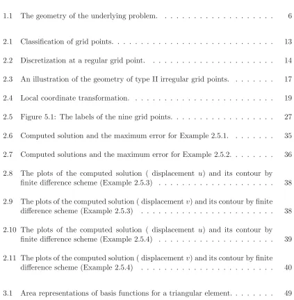
1.1 The geometry of the underlying problem. . . 6
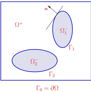
2.1 Classification of grid points. . . 13
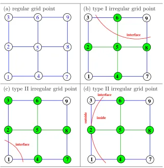
2.2 Discretization at a regular grid point. . . 14
2.3 An illustration of the geometry of type II irregular grid points. . . 17
2.4 Local coordinate transformation. . . 19
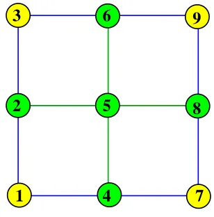
2.5 Figure 5.1: The labels of the nine grid points. . . 27
2.6 Computed solution and the maximum error for Example 2.5.1. . . 35
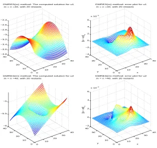
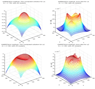
2.7 Computed solutions and the maximum error for Example 2.5.2. . . 36
2.8 The plots of the computed solution ( displacement u) and its contour by finite difference scheme (Example 2.5.3) . . . 38
2.9 The plots of the computed solution ( displacementv) and its contour by finite difference scheme (Example 2.5.3) . . . 38
2.10 The plots of the computed solution ( displacement u) and its contour by finite difference scheme (Example 2.5.4) . . . 39
2.11 The plots of the computed solution ( displacementv) and its contour by finite difference scheme (Example 2.5.4) . . . 40
3.1 Area representations of basis functions for a triangular element. . . 49
3.3 A global basis function centered at a nodal point. . . 54
3.4 A typical interface triangle ∆ABC . . . 55
3.5 Local basis functions foru and v (λ+= 80.,λ−= 160.,ν+=.35, ν−=.15 ). 61 3.6 A global basis function for u and its contour plot (λ+ = 40., λ− = 90., ν+=.35, ν−=.15 ). . . 61
3.7 A global basis function for v and its contour plot (λ+ = 40., λ− = 90., ν+=.35, ν−=.15 ). . . 62
3.8 A typical triangular element. . . 64
3.9 A typical boundary element of domain Ω. . . 68
3.10 Coordinate transformation I. . . 70
3.11 Coordinate transformation II. . . 70
3.12 The plots of the computed solution ( displacement u) and its contour by FEM (Example 3.7.1). . . 78
3.13 The plots of the computed solution ( displacementv) and its contour by FEM (Example 3.7.1). . . 79
3.14 The plots of the computed solution ( displacement u) and its contour by FEM (Example 3.7.2). . . 80
3.15 The plots of the computed solution ( displacementv) and its contour by FEM (Example 3.7.2). . . 80
3.16 The plots of the computed solution ( displacement u) and its contour by FEM (Example 3.7.3). . . 81
3.17 The plots of the computed solution ( displacementv) and its contour by FEM (Example 3.7.3). . . 81
3.18 The plots of the computed solution ( displacement u) and its contour by FEM (Example 3.7.4). . . 82
A.1 The numbering strategy of the nodal points and elements . . . 86
Introduction
1.1
An overview of interface problems
Many applied problems involve interfaces, such as Stokes flow with moving interfaces [56,
65], Stefen problems, which is often used to describe free boundary problems in heat-transfer,
phase transition problems and multi-phase flow, models of ice-melting and glaciation [61],
Hele-Shaw flow [45], bubble simulations in incompressible two-phase flow [12], elasticity
problems with interfaces in materials science [69, 85, 92], problems of multiple phase elastic
materials separated by phase interfaces [69, 85], the microstructural evolution of precipitates
in an elastic matrix due to the diffusion of concentration and in the morphological instability
due to stress-driven surface diffusion in solid thin films [6, 43, 51]. Interface problems also
exist in biological fluid dynamics which may involve the complex geometry and frequently
the interaction of fluids with moving elastic structures. The study of blood flow in flexible
tubes, cell dynamics and motility, and the functioning of various physiological mechanisms
require solving interface problems [23, 29, 30, 31, 32, 33, 52, 67, 76, 73, 68, 74].
Mathematically, interface problems usually lead to differential equations with
discon-tinuous or non-smooth solutions across interfaces. Many numerical methods designed for
smooth solutions do not work efficiently for interface problems.
Interface problems of our interest may have one or more of the following properties:
• The coefficients of the differential equations may be discontinuous across the interfaces.
• The solutions and their derivatives may be discontinuous across the interfaces.
• There may be discontinuous or singular sources, or dipoles along interfaces.
• The interfaces may be fixed or moving.
• There may be more than one interface.
The curved interface in interface problems brings up several substantial difficulties in
the development and analysis of numerical schemes:
• Due to the non-smoothness of the solutions across the interface, many conven-tional discretization scheme will not work efficiently.
• Generally interfaces can be arbitrary and complicated, and analytical expres-sions for them are rarely available.
• It is difficult to perform convergence analysis for interface problems in the con-ventional way.
• The system of discrete equations using finite difference scheme may not be sym-metric or positive definite. This structure of the system will bring difficulty to
use efficient solvers.
Over years, many numerical methods for interface problems have been developed, in
which Cartesian grid based methods take advantage in dealing with the moving interface
problems. Below is an incomplete brief review related to this thesis.
• The immersed boundary (IB) method: The immersed boundary method [68, 75, 78] was developed by Peskin in 1977 to model the blood flow in the heart [73,
74, 76]. Peskin’s immersed boundary method has been applied successfully to
many fluid and biological problems [29, 32, 67, 70]. This method has become a
standard numerical method for interface problems that involve singular forces
for non-smooth but continuous quantities. To improve the accuracy, Lai and
Peskin in [54] developed a nearly second-order accurate scheme which has less
numerical viscosity to simulate the flow past a circular cylinder. The scheme is
therefore a better choice for the simulation of high Reynolds number flows with
immersed boundaries. In [19] Cortez and Minion proposed another high order
scheme using the smoothed blob projection to compute the force. However using
a delta function formulation in [19, 54] smears out the solution on a thin finite
band about the interface.
• The ghost fluid method (GFM): The ghost fluid method was first presented by Fedkiw et al in [34]. The GFM is a sharp interface method and it has been
applied to multiphase incompressible flow and two phase incompressible flames
simulations. However this method is only first order accurate in the maximum
norm.
• The finite element method (FEM) using body-fitted grid: The finite element method has been widely used in solving structural, mechanical, heat transfer,
and fluid dynamics problems as well as problems of other disciplines [5, 9, 15,
24, 48, 57, 66, 86, 91, 93, 94, 95]. This approach has the advantage of a
rigor-ous theoretical framework and many optimized commercial implementations. It
has been applied to many interface problems. For example, Chen and Zou in
[14] applied the finite element method to elliptic interface problems using body
fitted grids. Traditional finite element method involves mesh generation, which
is usually expensive especially for moving interface problems. Although it is a
popular method, the FEM involves substantially more complicated date
struc-ture than do Cartesian-grid methods. The complicated date strucstruc-ture increase
the complexity and cost of many parts of the solution process, especially in the
linear algebra.
• The immersed interface method: The immersed interface method (IIM) origi-nally developed by LeVeque and Li [55, 58, 62] is one of most efficient methods
used to solve the interface problems. It has been applied to many problems
ranging from one, two, three dimensional problems, elliptic, parabolic,
many applications such as in solid mechanics and fluid mechanics and so on.
IIM has been proved to have better accuracy than Peskin’s immersed boundary
method [29, 67, 68, 75, 78] using a discrete delta function. IIM is a Cartesian grid
based method. By using Cartesian grids, there are several advantages in
solv-ing interface problems, or problems with complicated geometries, or topological
changes [46, 64, 79, 88]. First this method costs nothing in grid generation.
Sec-ondly, using Cartesian grids we can take advantage of many software packages or
methods developed for Cartesian grids, for example, fast Poisson solvers,
Claw-pack, AmrclawClaw-pack, the level set method [50, 71, 72, 80, 81], algebraic multigrid
solvers [1, 2, 10], and many others. Moreover, the level set method works best
with Cartesian grids.
• Level set method (LSM): The level set method [72, 80, 81] was first proposed by S. Osher and J. A. Sethian, has been successfully used to treat a number of
moving interface/boundary problems [13]. It can handle problems with
topo-logical changes, and problems in three dimensions easily. Due to its simplicity
in implementation, we use the level set method in Chapter 3 to represent the
interface.
• The immersed finite element (IFE) method: The immersed finite element method was first presented by Li in [61]. This method is also called finite-element
immersed interface method, which uses Cartesian grids for solving differential
equations with discontinuities in the coefficients across one or several arbitrary
interfaces in the solution domain. In [64], Li, Tao and Wu developed the IFE
method for an elliptic problem with boundary conditions. Both non-conforming
and conforming finite element spaces are considered in [64], and Li et al in [64]
proved that the corresponding interpolation functions are second order accurate
in the maximum norm and that the conforming finite element is convergent. The
basic idea of the IFE method is to form a partition which is independent of
inter-face so that partitions with simple and efficient structures, such as a Cartesian
partition can be used to solve an interface problem with a rather complicate or
varying interface. For a triangulation in uniform Cartesian grids, the triangles
and interface triangles. The local nodal basis functions in a non-interface
tri-angle will be the standard linear polynomials and the local basis functions in
an interface triangle can be piece-wise linear polynomials obtained by the given
interface conditions. In this thesis the immersed finite element method for
elas-ticity problems with interfaces will be developed in Chapter 3.
1.2
Elasticity problems with interfaces
Elasticity problems of multiple phase elastic materials separated by phase interfaces often
arise in materials science [69, 85]. Two important examples of such problems occur in the
microstructural evolution of precipitates in an elastic matrix due to the diffusion of
concen-tration and in the morphological instability due to stress-driven surface diffusion in solid
thin films, cf. e.g., [6, 43, 51] and the references therein. The understanding of these physical
processes is crucial to improve material stability properties, and in turn to develop new and
advanced materials that have applications in automobile manufacture, aircraft industries,
and modern communication technologies. However, solving such elasticity problems are
often very difficult due to complicated geometries, multiple components, and nonlinearities
that appear in these problems. For these reasons, there has been a great interest recently,
in all materials science, scientific computing, and applied mathematics communities, in
de-veloping efficient and accurate numerical techniques for elasticity problems with interfaces
separating multiple phases.
In this thesis, we consider a two-dimensional problem that can arise from many modeling
situations such as two-phase elastic plates in the setting of plane strain or plane stress [16,
40, 83]. We assume that the elastic material occupies a bounded domain Ω ⊂ R2 with
boundary Γ0 = ∂Ω. For our computational purpose, we assume that the domain Ω is
00000000000 00000000000 00000000000 00000000000 00000000000 00000000000
11111111111 11111111111 11111111111 11111111111 11111111111
11111111111000000
000000 000000 000000 000000 000000 000000 000000 000000
111111 111111 111111 111111 111111 111111 111111 111111 111111
Ω
−2
Ω
+Γ
1Γ
2Ω
−1
Γ0
=
∂
Ω
n
Figure 1.1: The geometry of the underlying problem.
The equilibrium equation, interface conditions on Γ, and the boundary conditions on Γ0
are:
∇ ·σ+F = 0 in Ω+∪Ω−, (1.1)
[u] = 0 on Γ, (1.2)
[σn] = 0 on Γ, (1.3)
u=u0 on Γ0, (1.4)
where σ is the stress tensor, F = (F1, F2)T : Ω → R2 is the body force which is known (a superscript T denotes the transpose), u = (u1, u2)T : Ω → R2 with u1 = u1(x, y) and
u2 =u2(x, y) is the displacement field, for a functionv, [v] =v+−v− denotes the jump of
v across the interface, n= (n1, n2)T is the unit normal vector to the interface Γ, pointing from the −phase to the + phase, and u0 is a given vector-valued function that represents
the displacement on the boundary Γ0. The jump condition (1.2) means thatuis continuous
across the interface. It indicates that the underlying material has no fracture.
We assume that the material is isotropic. So, in the setting of plane deformation, the
stress-strain relation is given by
=
(λ+ 2µ)∂u∂x1 +λ ∂u2
∂y µ
∂u1
∂y + ∂u2
∂x
µ
∂u1
∂y + ∂u2
∂x
λ∂u∂x1 + (λ+ 2µ)∂u∂y2
, (1.5)
where
ε= 1
2
∇u+ (∇u)T=
∂u∂x1 12
∂u1
∂y + ∂u2
∂x
1 2
∂u1
∂y + ∂u2
∂x
∂u2
∂y
(1.6)
is the linear strain,I is the 2×2 identity tensor,
µ= E
2(1 +ν) and λ=
Eν
(1 +ν)(1−2ν)
are the Lam´econstants, E is Young’s modulus, andν is Poisson’s ratio. ν is dimensionless
and typically ranges from 0.2 ∼ 0.49, and is around 0.3 for most materials (cf. [4, 44]).
Rubber has a Poisson ratio close to 0.5 and is therefore almost incompressible (its volume
remains almost constant, no matter how it is deformed). Cork, on the other hand, has a
Poisson ratio close to zero (no lateral contraction when stretched). Some bizarre materials
have ν <0 – if you stretch a round bar of such a material, the bar increases in diameter.
In modeling a two-phase elastic material, we assume that all the material parameters µ,
λ,E, andν are piecewise constants. In particular, we assume that the shear modulus and
Poisson’s ratio are given, respectively, by
µ=
µ+ in Ω+
µ− in Ω−
and ν =
ν+ in Ω+
ν− in Ω−
,
where all µ+,µ−,ν+,ν− are positive constants.
There exist several numerical methods for solving general elasticity problems that do not
involve interfaces. Among them, the finite element method and the boundary integral or
boundary element method appear to be very successful, cf. e.g., [7, 77, 96] and the references
therein. However, in treating moving interface problems, the use of fixed Cartesian grids
often shows advantages in practical computations [46, 64, 79, 88]. It is therefore desirable to
develop new, efficient methods based on fixed Cartesian grids for our underlying elasticity
problems with interfaces. This is our primary goal of the work. Our idea is to use the
difference or finite element scheme for the elasticity problem with an interface. This is a
natural strategy, since the geometrical complexity of the problem is local.
Since with a uniform Cartesian grid, the interface is typically not aligned with the
grid but rather cuts between grid points. Thus, for grid points near the interface, the
stencil of a standard finite difference scheme will contain points from both sides of the
interface. Due to the non-smoothness of the solution across the interface, differentiating
it using standard finite difference schemes will not produce accurate approximations to its
derivatives. The cross derivative terms in the differential equations need special treatments
in the discretization on the grid points near or on the interface. The curved interface in the
underlying problem brings up some substantial difficulties in the development and analysis
of numerical schemes.
1.3
Outline of the thesis
The main task of this thesis is the development of the immersed interface method and
the immersed finite element method to the underlying elasticity problems with interfaces.
The thesis is organized as follows: In Chapter 2 we develop a finite difference scheme for
elasticity problems with interfaces. The key in our method is to utilize the local coordinate
transformation to carefully analyze the relations of quantities from one side to the another.
Such relations shall lead us to find accurate finite difference schemes for grid points near
or on the interface. Numerical examples will show that the immersed interface method
is of second order accuracy. Chapter 3 will present the immersed finite element method
for elasticity problems with interfaces. The basis functions for non-interface elements and
interface elements will be presented in this chapter. Some numerical examples will also
be presented and compared with the results by finite difference method in Chapter 2. In
Chapter 4, we draw conclusions and outline our future work. In Appendix, two Fortran
90 modules are given for Chapter 3. Module geometry lib in A.1 contains the subroutine
that forms the coordinates and node vector for a uniform 3-node triangle in a rectangular
IIM using Finite Difference for Elasticity Problems
with Interfaces
In this chapter we will develop an immersed interface method for solving linear elasticity
problems with two phases separated by an interface. For the problem of interest, the
underlying elasticity modulus is a constant in each phase but vary from phase to phase.
The basic goal here is to design an efficient numerical method using a fixed Cartesian grid.
The application of such a method to problems with moving interfaces driving by stresses
has a great advantage: no re-meshing is needed. A local optimization strategy is employed
to determine the finite difference equations at grid points near or on the interface. The
bi-conjugate gradient method and the GMRES with preconditioning are both implemented
to solve the resulting linear systems of equations and compared. Numerical results are
presented to show that the method is second-order accurate.
In Section 2.1, we describe our algorithm. In Section 2.2, we introduce local coordinate
transformation that is essential to the development of our method. In Section 2.3, we
describe interface relations. In Section 2.4, we derive the finite difference scheme for irregular
grid points. The linear solvers are also discussed. In Section 2.5, we present our numerical
results and the results indicate our method is second-order accurate. Section 2.6 summarizes
the IIM using the finite difference.
2.1
Description of the Algorithm
For the convenience of debugging, we actually allow the tractionσn to have a finite jump
across the interface Γ:
[σn] =T = [φ, ψ]T on Γ. (2.1)
In this case (1.3) will be a special case of (2.1).
We let f = −F1/(µ+λ) and g = −F2/(µ+λ), and equations (1.1) and (1.3) can be
written as
2(1−ν)∂
2u1
∂x2 + (1−2ν)
∂2u1
∂y2 +
∂2u2
∂x∂y =f(x, y), (2.2)
(1−2ν)∂
2u 2
∂x2 + 2(1−ν) ∂2u2
∂y2 +
∂2u1
∂x∂y =g(x, y), (2.3)
2µ
1−2ν
(1−ν)∂u1
∂x +ν
∂u2
∂y
n1+µ
∂u1 ∂y + ∂u2 ∂x n2 Γ
=φ, (2.4)
µ ∂u1 ∂y + ∂u2 ∂x
n1+ 2µ
1−2ν
ν∂u1
∂x + (1−ν)
∂u2
∂y
n2
Γ
=ψ, (2.5)
where [·] is defined as the jump of the quantity between the outside and the inside of the
interface.
For simplicity, we assume that the domain Ω is a square: Ω = (a, b) ×(c, d) with
d−c=b−a. Letn≥1 be an integer and h= (b−a)/n= (d−c)/n. Let
xi =a+ih, yj =c+jh, i, j= 0,· · · , n.
We wish to solve the problem using a finite difference method on the uniform Cartesian
grid. Our result will be a finite difference scheme of the form k
αk(U1)i+ik,j+jk+
k
βk(U2)i+ik,j+jk = fij+Cij1,
k
γk(U1)i+ik,j+jk+
k
δk(U2)i+ik,j+jk = gij +Cij2,
(2.6)
coefficients. Each sum over k in (2.6) involves only finite number of grid points that are
centered at (xi, yj) (at most nine grid points are involved in our algorithm), all ik, jk ∈ {−1,0,1}. The coefficients αk, βk, γk, and δk and the indices ik, jk will depend on (i, j). We omit the dependency for simplicity. By finding these coefficients properly, we can obtain
a second-order accurate finite difference scheme.
2.1.1 Classification of grid points
Before we explain the finite difference scheme, we classify all grid points into two categories:
regular and irregular. We say a grid point (xi, yj) is regular (Figure 2.1 (a)) if the interface Γ does not cut through any points in the standard nine point stencil centered at (xi, yj). We say a grid point is irregular, if it is not regular. An irregular grid point is further classified as type I, if the interface crosses the five point stencil centered at this point (Figure 2.1
(b)), and type II, if otherwise (Figure 2.1 (c) and (d)).
At a regular grid point (Figure 2.1 (a)), we use the standard central finite difference
scheme. At an irregular grid point (see Figure 2.1 (b)–(d)), we derive a finite difference
scheme according to how the interface cuts through the five-point stencil.
2.1.2 Discretization at regular grid points
At a regular grid point (xi, yj), we have the following approximations of the second-order partial derivatives for a given smooth function u
uxx(xi, yj) =
u(xi−1, yj)−2u(xi, yj) +u(xi+1, yj)
h2 +O(h
2),
uyy(xi, yj) =
u(xi, yj−1)−2u(xi, yj) +u(xi, yj+1)
h2 +O(h
2),
uxy(xi, yj) =
u(xi+1, yj+1) +u(xi−1, yj−1)−u(xi−1, yj+1)−u(xi+1, yj−1)
4h2 +O(h
(a) regular grid point (b) type I irregular grid point
6
4 3
8 2
1 7
5
9
interface
1 2 3
4 5 6
7 8 9
(c) type II irregular grid point (d) type II irregular grid point
1 2 3
4 5 6
7 8 9
interface
1 2 3
4 5 6
7 8 9
outside
interface
inside
cf. Figure 2.1.2. These lead to the following discretization of (2.2) and (2.3):
2(1−ν)
h2
(U1)i−1,j+ (U1)i+1,j
+1−2ν
h2
(U1)i,j−1+ (U1)i,j+1
−2(3−4ν)
h2 (U1)i,j +
1 4h2
(U2)i+1,j+1+ (U2)i−1,j−1
−(U2)i−1,j+1−(U2)i+1,j−1
=fij,
1−2ν h2
(U2)i−1,j+ (U2)i+1,j
+2(1−ν)
h2
(U2)i,j−1+ (U2)i,j+1
−2(3−4ν)
h2 (U2)i,j +
1 4h2
(U1)i+1,j+1+ (U1)i−1,j−1
−(U1)i−1,j+1−(U1)i+1,j−1
=gij,
(2.7)
where (U)i,j stands for the approximation of u(xi, yj), and in this case Cij1 = Cij2 = 0, cf. (2.6).
1
2
3
4
5
6
7
8
9
Figure 2.2: Discretization at a regular grid point.
2.1.3 Discretization at type I irregular grid points
Following [55] and [58], we use a nine-point stencil for u1 and u2 in both equations of
andu2(xi+ik, yj+jk) in (2.6) and use the Taylor expansion at (x∗i, yj∗) for each term in order to set up a system of equations for the coefficients. Since the solution from both sides is
involved, we use the superscript− and + to denote the limiting values of a function from
one side or the other. For example, if the point (xi, yj) is located inside the interface, then we can expandu(xi, yj) to get
u(xi, yj) = u−+u−x(xi−x∗i) +u−y(yj −yj∗) + 1 2u
−
xx(xi−x∗i)2
+1 2u
−
yy(yj−y∗j)2+u−xy(xi−xi∗)(yj−yj∗) +O(h3).
If we do such expansion at each grid point used in the finite difference equations in (2.6),
then the local truncation errorsTij1 and Tij2 (for the first and second equation respectively) can be expressed as a linear combination of all the values u±1,u±1x,u±1y,u±1xx,· · ·,u±2yy, and
u±2xy.
Next, we express all the values from + side, u+1, u+1x, u+1y, · · ·, u+2yy, u+2xy, in terms of the values on the − side, u−1,u−1x,u−1y, · · ·, u−2xx,u−2yy,u−2xy. To do so, we need to use the interface conditions,
u+1 =u−1, u+2 =u−2, (2.8)
2µ+
1−2ν+
(1−ν+)(u1)x++ν+(u2)+y
n1+µ+
(u1)+y + (u2)+x
n2
= 2µ − 1−2ν−
(1−ν−)(u1)x−+ν−(u2)−y
n1
+µ−
(u1)−y + (u2)−x
n2+φ, (2.9)
µ+
(u1)+y + (u2)+x
n1+ 2µ
+
1−2ν+
ν+(u1)+x + (1−ν+)(u2)+y
n2
=µ−
(u1)−y + (u2)−x
n1+ 2µ
− 1−2ν−
ν−(u1)−x
+ (1−ν−)(u2)−y
n2+ψ. (2.10)
To obtain all the coefficients αk,βk,γk, andδk in the finite difference equations (2.6), more interface relations are needed. Differentiating the above equations and manipulating the
do so, it is very convenient to first perform a local coordinate transformation in the normal
directionξ, and the tangential direction η of Γ at (x∗i, y∗j).
Once the local truncation errorsTij1 andTij2 are expressed as a linear combination of the values from just one side, say u−1,u−1x,u−1y,u−1xx,u−1yy,u−1xy,u−2,u−2x,u−2y,u−2xx,u−2yy,u−2xy, we must require that the coefficient of each of these terms to vanish in order to match the
partial differential equation up to second order derivative terms. This gives us a system
of twelve linear equations from the first and second finite difference equations respectively.
Nine-point stencil will be used to obtain a solvable system, see Section 2.4 for all these
derivations.
2.1.4 Discretization at type II irregular grid points
For a type II irregular grid point (cf. Figure 2.1 (c) and (d)), we use
• five-point stencil foru1and seven-point or four-point stencil for the cross deriva-tive ofu2 in the first equation, and
• five-point stencil foru2and seven-point or four-point stencil for the cross deriva-tive ofu1 in the second equation.
Therefore equations (2.2) and (2.3) have the following form:
2(1−ν)
h2
(U1)i−1,j+ (U1)i+1,j
+1−2ν
h2
(U1)i,j−1+ (U1)i,j+1
−2(3−4ν)
h2 (U1)i,j+
k
βk(U2)i+ik,j+jk =fij, (2.11)
1−2ν h2
(U2)i−1,j+ (U2)i+1,j
+2(1−ν)
h2
(U2)i,j−1+ (U2)i,j+1
−2(3−4ν)
h2 (U2)i,j+
k
γk(U1)i+ik,j+jk =gij. (2.12)
for a smooth function u to derive our finite difference scheme
uxy =
u(1)−u(2)−u(4)+u(5)
h2 +O(h) (2.13)
= u
(2)−u(3)−u(5)+u(6)
h2 +O(h) (2.14)
= u
(4)−u(5)−u(7)+u(8)
h2 +O(h) (2.15)
= u
(5)−u(6)−u(8)+u(9)
h2 +O(h), (2.16)
whereu(i)denotesuvalue at the point numberediin Figure 2.1. Which formula from (2.13)
∼(2.16) to use depends on how the interface crosses the nine -point stencil. In the specific case in Figure 2.1 (d), we use the expansion (2.15) or (2.16), where points numbered (4) to
(9) are in the same side of the interface. However, when one grid point is on the other side
of the other eight grid points in the nine-point stencil as shown in Figures 2.3 (a) and (b),
we apply the following formula for a smooth functionu. In this case we have
uxy =
u(2)−u(3)+u(4)−2u(5)+u(6)−u(7)+u(8)
2h2 +O(h
2) (2.17)
= u
(1)−u(2)−u(4)+ 2u(5)−u(6)−u(8)+u(9)
2h2 +O(h
2). (2.18)
Whether we use (2.17) or (2.18) depends on the geometry. We use, for example, the formula
(2.17) in Figure 2.3 (a), and (2.18) in Figure 2.3 (b).
1 2 3
4 5 6
7 8 9
interface
2 3
4 5 6
7 8 9
1
interface
(a) (b)
2.2
Transformations of Local Coordinates
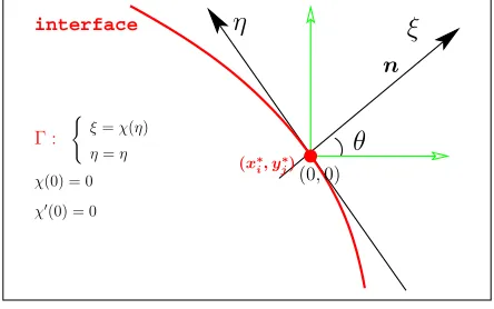
For each type I irregular point (xi, yj), we need to find a point (x∗i, yj∗) on the interface. We usually take this point as the projection of (xi, yj) on the interface if the interface is smooth at this point. Otherwise we can take any point on the interface where the interface
is smooth.
After (x∗i, y∗j) is selected, we apply the local coordinate transformation at this point. Let θbe the angle between the x−axis and the normal direction, pointing in the direction
of the + side, cf. Figure 2.4. The transformation is defined as follows:
ξ = (x−x∗i) cos(θ) + (y−yj∗) sin(θ),
η = −(x−x∗i) sin(θ) + (y−yj∗) cos(θ).
(2.19)
Under this local coordinate transformation, the governing equations in (2.2) and (2.3)
be-come
(cos2θ+ 1−2ν)u1ξξ−2 sinθcosθu1ξη+ (sin2θ+ 1−2ν)u1ηη
+ sinθcosθu2ξξ+ (cos2θ−sin2θ)u2ξη−sinθcosθu2ηη =f, (2.20)
(sin2θ+ 1−2ν)u2ξξ+ 2 sinθcosθu2ξη+ (cos2θ+ 1−2ν)u2ηη
+ sinθcosθu1ξξ+ (cos2θ−sin2θ)u1ξη−sinθcosθu1ηη =g, (2.21)
wheref =f(x, y) = ˜f(ξ, η), g=g(x, y) = ˜g(ξ, η) for simplicity.
2.3
Interface Relations
We consider a fixed point (x∗i, y∗j) and define a new ξ-η coordinate system based on the directions normal and tangential to Γ at this point using the formulas (2.19). In a
neigh-borhood of this point, the interface can be parameterized as ξ =χ(η), η=η. Notice that
χ(0) = 0 andχ(0) = 0 provided that the interface is smooth at (x∗i, y∗j). We need to express all the quantities with the superscript + in terms of those quantities with the superscript
interface
n
ξ
η
θ
Γ :χ(0) = 0
χ(0) = 0
ξ=χ(η) η=η
(0,0)
(x∗i, y∗j)
Figure 2.4: Local coordinate transformation.
First, using the same approach as that in [55] and [58], we easily get the following jump
conditions foru1 and u2,
u+1(χ(η), η)|η=0 =u−1(χ(η), η)|η=0, (2.22)
u+2(χ(η), η)|η=0 =u−2(χ(η), η)|η=0, (2.23)
[u1ξ]χ+ [u1ηη] = 0, [u2ξ]χ+ [u2ηη] = 0. (2.24)
The jump (2.24) can be rewritten as
u+1ηη =u−1ηη+χu−1ξ−χu+1ξ, (2.25)
u+2ηη =u−2ηη+χu−2ξ−χu+2ξ. (2.26)
Notice that, in the local coordinate system, the unit normal at any point (χ(η), η) on
the interface is
n= (n1,n2)T =
1
1 + (χ(η))2,
−χ(η)
1 + (χ(η))2 T
. (2.27)
Therefore, at (x∗i, y∗j), or (0,0) in the local coordinate system, we have
n1η|η=0 = −
χ(η)χ(η) (1 + (χ(η))2)32
η=0
,
n2η|η=0 = −
χ(η)
1 + (χ(η))2
η=0 + (χ
(η))2χ(η)
(1 + (χ(η))2)32
η=0
Recalling thatχ(0) = 0 andχ(0) = 0, we have, at (x∗i, y∗j), or (0,0) in the local coordinate system, that
n1 = 1, n2 = 0, (2.28)
n1η = 0, n2η =−χ(0). (2.29)
In the x-y coordinate system, we have n= (n1, n2)T. The relation between (n1, n2)T and (n1,n2)T is determined by
n1 =n1∗cosθ−n2∗sinθ,
n2 =n1∗sinθ+n2∗cosθ.
Hence, by (2.28) and (2.29), we obtain
n1= cosθ, n2 = sinθ, (2.30)
n1η|η=0=n1η|η=0cosθ−n2η|η=0sinθ=χ(0) sinθ, (2.31)
n2η|η=0=n1η|η=0sinθ+n2η|η=0cosθ=−χ(0) cosθ. (2.32)
These relations will be used to derive the interface relations for u+1ξη andu+2ξη.
The following result is required to find the interface relations so every quantity from
u+1ξ, u+2ξ, u+1ξη, u+2ξη, u+1ξξ and u2+ξξ, can be expressed in terms of u−1, u−1x, u−1y, u−1xx, u−1yy,
u−1xy,u−2,u−2x,u−2y,u−2xx,u−2yy, and u−2xy. Its proof is trivial, and is omitted.
Lemma 4.1. If Det=
aa1121 aa1222
= 0, then the system of linear equations
a11x+a12y = b11z1+b12z2+· · ·+b1nzn
a21x+a22y = b21z1+b22z2+· · ·+b2nzn has the unique solution
x= Det1
bb1121 aa1222
z1+
bb1222 aa1222
z2+· · ·+
bb12nn aa1222
zn
y= Det1
aa1121 bb1121
z1+
aa1121 bb1222
z2+· · ·+
aa1121 bb12nn
2.3.1 Interface relations for u+1ξ and u+2ξ
Rewrite the interface conditions (2.9) and (2.10) as follow:
n1(α+u+1x+β+u+2y) +n2µ+(u+1y+u+2x)
=n1(α−u−1x+β−u−2y) +n2µ−(u−1y +u−2x) +φ(x, y),
n1µ+(u+1y+u+2x) +n2(β+u+1x+α+u+2y)
=n1µ−(u−1y+u−2x) +n2(β−u−1x+α−u−2y) +ψ(x, y),
wheren= (n1, n2)T = (n1(ξ, η), n2(ξ, η))T is the unit normal to the interface and
α+= 2µ
+
1−2ν+(1−ν
+), β+= 2µ+
1−2ν+ν
+,
α−= 2µ
−
1−2ν−(1−ν
−), β−= 2µ− 1−2ν−ν
−.
Notice that
∂u1
∂x =u1ξξx+u1ηηx = cos(θ)u1ξ−sin(θ)u1η,
∂u1
∂y =u1ξξy+u1ηηy = sin(θ)u1ξ+ cos(θ)u1η,
∂u2
∂x =u2ξξx+u2ηηx = cos(θ)u2ξ−sin(θ)u2η,
∂u2
∂y =u2ξξy+u2ηηy = sin(θ)u2ξ+ cos(θ)u2η.
Thus, in the local ξ-η coordinate system, we have
(n1α+cosθ+n2µ+sinθ)u+1ξ+ (−n1α+sinθ+n2µ+cosθ)u+1η
+(n1β+sinθ+n2µ+cosθ)u+2ξ+ (n1β+cosθ−n2µ+sinθ)u+2η
= (n1α−cosθ+n2µ−sinθ)u−1ξ+ (−n1α−sinθ+n2µ−cosθ)u−1η
+(n1β−sinθ+n2µ−cosθ)u−2ξ+ (n1β−cosθ−n2µ−sinθ)u−2η
+φ(ξ, η), (2.33)
(µ+n1sinθ+n2β+cosθ)u+1ξ+ (n1µ+cosθ+n2α+sinθ)u+2ξ
+(n1µ+cosθ−n2β+sinθ)u+1η + (−µ+n1sinθ+n2α+cosθ)u+2η
= (µ−n1sinθ+n2β−cosθ)u−1ξ+ (n1µ−cosθ+n2α−sinθ)u−2ξ
+ψ(ξ, η). (2.34)
Using the fact that n1 = cosθ,n2 = sinθ at (0,0) in the local coordinate system and
the jump conditions (2.22) and (2.23), we can solve for u+1ξ and u+2ξ from equations (2.33) and (2.34) in terms of u−1,u−1ξ,· · ·,u−2ξη. In fact, using (2.30) we can rewrite the equations (2.33) and (2.34) as
(α+cos2θ+µ+sin2θ)u1+ξ+ (β++µ+) sinθcosθu+2ξ
= (α−cos2θ+µ−sin2θ)u1−ξ+ (−α−+µ−) sinθcosθu−1η
−(−α++µ+) sinθcosθu+1η−(β+cos2θ−µ+sin2θ)u+2η
+(β−+µ−) sinθcosθu−2ξ+ (β−cos2θ−µ−sin2θ)u−2η
+φ(ξ, η), (2.35)
(µ++β+) sinθcosθu+1ξ+ (µ+cos2θ+α+sin2θ)u+2ξ
= (µ−+β−) sinθcosθu−1ξ+ (µ−cos2θ+α−sin2θ)u−2ξ
−(µ+cos2θ−β+sin2θ)u1+η−(−µ++α+) sinθcosθu+2η
+(µ−cos2θ−β−sin2θ)u1−η+ (−µ−+α−) sinθcosθu−2η
+ψ(ξ, η). (2.36)
Since u+1η =u−1η and u+2η =u−2η, the right hand sides of (2.35) and (2.36) become
b1 = (α−cos2θ+µ−sin2θ)u−1ξ
+[(α+−α−)−(µ+−µ−)] sinθcosθu−1η
+(β−+µ−) sinθcosθu−2ξ
+[(µ+−µ−) sin2θ−(β+−β−) cos2θ]u−2η+φ(ξ, η),
b2 = (µ−+β−) sinθcosθu−1ξ
+[(β+−β−) sin2θ−(µ+−µ−) cos2θ]u−1η
+(µ−cos2θ+α−sin2θ)u−2ξ
+[(µ+−µ−)−(α+−α−)] sinθcosθu−2η+ψ(ξ, η).
Let
a11= cos2θα++ sin2θµ+, a12= (β++µ+) sinθcosθ,
The determinant of the coefficient matrix for the linear system (2.35) and (2.36) is
aa1121 aa1222
=
cos
2θα++ sin2θµ+ (β++µ+) sinθcosθ
(µ++β+) sinθcosθ µ+cos2θ+α+sin2θ
=α+µ+.
Since
α+µ+= 2(µ
+)2
1−2ν+(1−ν
+)= 0, (2.37)
the system (2.35) and (2.36) has the unique solution
u+1ξ = 1
α+µ+
bb12 aa1222
= 1
α+µ+(a22b1−a12b2), (2.38)
u+2ξ = 1
α+µ+
aa1121 bb12
= 1
α+µ+(a11b2−a21b1. (2.39)
Consequently, the values u+1ξ and u+2ξ can be expressed in terms of u1−, u−1ξ, · · ·, u−2ξη. Moreover, plugging (2.38) and (2.39) into (2.25) and (2.26), we can also express u+1ηη and
u+2ηη in terms of those values in the −side.
2.3.2 Interface relations for u+1ξη and u+2ξη
To find the interface relations for u+1ξη and u+2ξη, we differentiate (2.33) and (2.34) with respect to η. After some calculations, we obtain the following system of linear equations
about u+1ξη andu+2ξη
A11u+1ξη+A12u+2ξη =B1,
A21u+1ξη+A22u+2ξη =B2,
(2.40)
where the coefficients A11, A12, A21, A22 are given by
A11=n1α+cosθ+n2µ+sinθ, A12=n1β+sinθ+n2µ+cosθ,
A21=n1µ+sinθ+n2β+cosθ, A22=n1µ+cosθ+n2α+sinθ.
ofu−1,u−1ξ,· · ·,u−2ξη, the valuesB1andB2 can also be expressed in terms of these quantities as well. So we set
B1 = b11u−1 +b21u−1ξ+b13u−1η+b14u−1ξξ+b15u−1ηη+b16u−1ξη
+b17u−2 +b18u−2ξ+b19u−2η+b101 u−2ξξ+b111u−2ηη+b112u−2ξη +b10,
B2 = b21u−1 +b22u−1ξ+b23u−1η+b24u−1ξξ+b25u−1ηη+b26u−1ξη
+b27u−2 +b28u−2ξ+b29u−2η+b102 u−2ξξ+b211u−2ηη+b212u−2ξη +b20.
Since n1 = cosθ and n2 = sinθ, the determinant of the coefficient matrix of the system
(2.40) is
DET =
AA1121 AA1222
= cos
2θα++ sin2θµ+ (β++µ+) sinθcosθ
(µ++β+) sinθcosθ µ+cos2θ+α+sin2θ
= α+µ+= 0.
Thus, from Lemma 4.1, the solution to (2.40) is
u+1ξη = 1
DET
b
1 1 A12
b21 A22
u−1 + 1
DET
b
1 2 A12
b22 A22
u−1ξ
+ 1 DET b 1 3 A12
b23 A22
u−1η+ 1
DET
b
1 4 A12
b24 A22
u−1ξξ
+ 1 DET b 1 5 A12
b25 A22
u−1ηη+ 1
DET
b
1 6 A12
b26 A22
u−1ξη
+ 1 DET b 1 7 A12
b27 A22
u−2 + 1
DET
b
1 8 A12
b28 A22
u−2ξ
+ 1 DET b 1 9 A12
b29 A22
u−2η+ 1
DET
b
1 10 A12
b210 A22
u−2ξξ
+ 1 DET b 1 11 A12
b211 A22
u−2ηη+ 1
DET
b
1 12 A12
b212 A22
u−2ξη
+ 1 DET b 1 0 A12
b20 A22
u+2ξη = 1
DET
A11 b 1 1
A21 b21
u−1 + 1
DET
A11 b 1 2
A21 b22
u−1ξ
+ 1
DET
A11 b 1 3
A21 b23
u−1η+ 1
DET
A11 b 1 4
A21 b24
u−1ξξ
+ 1
DET
A11 b 1 5
A21 b25
u−1ηη+ 1
DET
A11 b 1 6
A21 b26
u−1ξη
+ 1
DET
A11 b 1 7
A21 b27
u−2 + 1
DET
A11 b 1 8
A21 b28
u−2ξ
+ 1
DET
A11 b 1 9
A21 b29
u−2η+ 1
DET
A11 b 1 10
A21 b210
u−2ξξ
+ 1
DET
A11 b 1 11
A21 b211
u−2ηη+ 1
DET
A11 b 1 12
A21 b212
u−2ξη
+ 1
DET
A11 b 1 0
A21 b20
. (2.42)
These are the desired relations.
2.3.3 Interface relations for u+1ξξ and u+2ξξ
From the differential equations (2.20) and (2.21), we have
(cos2θ+ 1−2ν+)u+1ξξ−2 sinθcosθu+1ξη+ (sin2θ+ 1−2ν+)u+1ηη
+ sinθcosθu+2ξξ+ (cos2θ−sin2θ)u+2ξη−sinθcosθu+2ηη−f+
= (cos2θ+ 1−2ν−)u−1ξξ−2 sinθcosθu−1ξη+ (sin2θ+ 1−2ν−)u−1ηη
+ sinθcosθu−2ξξ+ (cos2θ−sin2θ)u−2ξη−sinθcosθu−2ηη−f−, (2.43)
(sin2θ+ 1−2ν+)u+2ξξ+ 2 sinθcosθu+2ξη+ (cos2θ+ 1−2ν+)u+2ηη
+ sinθcosθu+1ξξ+ (cos2θ−sin2θ)u+1ξη−sinθcosθu+1ηη−g+