fastSTRUCTURE: Variational Inference of Population Structure in Large SNP Data Sets

(1)

HIGHLIGHTED ARTICLE

INVESTIGATION

fastSTRUCTURE: Variational Inference of Population

Structure in Large SNP Data Sets

Anil Raj,*,1_{Matthew Stephens,}†_{and Jonathan K. Pritchard*},‡

*Department of Genetics,‡Department of Biology, Howard Hughes Medical Institute, Stanford University, Stanford, California 94305, and†Departments of Statistics and Human Genetics, University of Chicago, Chicago, Illinois 60637

ABSTRACTTools for estimating population structure from genetic data are now used in a wide variety of applications in population genetics. However, inferring population structure in large modern data sets imposes severe computational challenges. Here, we develop efﬁcient algorithms for approximate inference of the model underlying the STRUCTURE program using a variational Bayesian framework. Variational methods pose the problem of computing relevant posterior distributions as an optimization problem, allowing us to build on recent advances in optimization theory to develop fast inference tools. In addition, we propose useful heuristic scores to identify the number of populations represented in a data set and a new hierarchical prior to detect weak population structure in the data. We test the variational algorithms on simulated data and illustrate using genotype data from the CEPH–Human Genome Diversity Panel. The variational algorithms are almost two orders of magnitude faster than STRUCTURE and achieve accuracies comparable to those of ADMIXTURE. Furthermore, our results show that the heuristic scores for choosing model complexity provide a reasonable range of values for the number of populations represented in the data, with minimal bias toward detecting structure when it is very weak. Our algorithm, fastSTRUCTURE, is freely available online athttp://pritchardlab.stanford.edu/structure.html.

I

DENTIFYING the degree of admixture in individuals and

inferring the population of origin of speciﬁc loci in these

individuals is relevant for a variety of problems in population

genetics. Examples include correcting for population stratiﬁ

-cation in genetic association studies (Pritchard and Donnelly

2001; Price et al. 2006), conservation genetics (Pearse and

Crandall 2004; Randi 2008), and studying the ancestry and

migration patterns of natural populations (Rosenberg et al.

2002; Reichet al.2009; Catchenet al.2013). With decreasing

costs in sequencing and genotyping technologies, there is an increasing need for fast and accurate tools to infer population structure from very large genetic data sets.

Principal components analysis (PCA)-based methods for

analyzing population structure, like EIGENSTRAT (Priceet al.

2006) and SMARTPCA (Pattersonet al.2006), construct

low-dimensional projections of the data that maximally retain the

variance-covariance structure among the sample genotypes.

The availability of fast and efﬁcient algorithms for singular

value decomposition has enabled PCA-based methods to be-come a popular choice for analyzing structure in genetic data sets. However, while these low-dimensional projections allow for straightforward visualization of the underlying popula-tion structure, it is not always straightforward to derive and interpret estimates for global ancestry of sample individuals from their projection coordinates (Novembre and Stephens 2008). In contrast, model-based approaches like

STRUC-TURE (Pritchardet al.2000) propose an explicit generative

model for the data based on the assumptions of Hardy-Weinberg equilibrium between alleles and linkage equilibrium between genotyped loci. Global ancestry estimates are then computed directly from posterior distributions of the model parameters, as done in STRUCTURE, or maximum-likelihood estimates of model parameters, as done in FRAPPE (Tang

et al.2005) and ADMIXTURE (Alexanderet al.2009).

STRUCTURE (Pritchard et al. 2000; Falushet al. 2003;

Hubisz et al.2009) takes a Bayesian approach to estimate

global ancestry by sampling from the posterior distribution over global ancestry parameters using a Gibbs sampler that appropriately accounts for the conditional independence relationships between latent variables and model parameters.

Manuscript received December 2, 2013; accepted for publication March 25, 2014; published Early Online April 2, 2014.

Available freely online through the author-supported open access option. Supporting information is available online athttp://www.genetics.org/lookup/suppl/ doi:10.1534/genetics.114.164350/-/DC1.

1_{Corresponding author: Stanford University, 300 Pasteur Dr., Alway Bldg., M337,}

(2)

However, even well-designed sampling schemes need to gener-ate a large number of posterior samples to resolve convergence and mixing issues and yield accurate estimates of ancestry proportions, greatly increasing the time complexity of infer-ence for large genotype data sets. To provide faster estimation, FRAPPE and ADMIXTURE both use a maximum-likelihood approach. FRAPPE computes maximum-likelihood estimates of the parameters of the same model using an expectation-maximization algorithm, while ADMIXTURE computes the same estimates using a sequential quadratic programming algorithm with a quasi-Newton acceleration scheme. Our goal in this article is to adapt a popular approximate infer-ence framework to greatly speed up inferinfer-ence of population structure while achieving accuracies comparable to STRUC-TURE and ADMIXSTRUC-TURE.

Variational Bayesian inference aims to repose the prob-lem of inference as an optimization probprob-lem rather than a sampling problem. Variational methods, originally used for approximating intractable integrals, have been used for a wide variety of applications in complex networks

(Hofman and Wiggins 2008), machine learning (Jordanet al.

1998; Blei et al. 2003), and Bayesian variable selection

(Logsdonet al.2010; Carbonetto and Stephens 2012).

Var-iational Bayesian techniques approximate the log-marginal likelihood of the data by proposing a family of tractable parametric posterior distributions (variational distribution)

over hidden variables in the model; the goal is then toﬁnd

the optimal member of this family that best approximates

the marginal likelihood of the data (seeModels and Methods

for more details). Thus, a single optimization problem gives us both approximate analytical forms for the posterior dis-tributions over unknown variables and an approximate esti-mate of the intractable marginal likelihood; the latter can be used to measure the support in the data for each model, and hence to compare models involving different numbers of populations. Some commonly used optimization algorithms for variational inference include the variational expectation-maximization algorithm (Beal 2003), collapsed variational

inference (Tehet al.2007), and stochastic gradient descent

(Sato 2001).

In Models and Methods, we brieﬂy describe the model underlying STRUCTURE and detail the framework for vari-ational Bayesian inference that we use to infer the

underly-ing ancestry proportions. We then propose a more ﬂexible

prior distribution over a subset of hidden parameters in the model and demonstrate that estimation of these hyperpara-meters using an empirical Bayesian framework improves the accuracy of global ancestry estimates when the underlying

population structure is more difﬁcult to resolve. Finally, we

describe a scheme to accelerate computation of the optimal variational distributions and describe a set of scores to help evaluate the accuracy of the results and to help compare

models involving different numbers of populations. In

Appli-cations, we compare the accuracy and time complexity of variational inference with those of STRUCTURE and AD-MIXTURE on simulated genotype data sets and demonstrate

the results of variational inference on a large data set gen-otyped in the Human Genome Diversity Panel.

Models and Methods

We now brieﬂy describe our generative model for

popula-tion structure followed by a detailed descrippopula-tion of the variational framework used for model inference.

Variational inference

Suppose we haveNdiploid individuals genotyped atL

bial-lelic loci. A population is represented by a set of allele

fre-quencies at theLloci,Pk2[0, 1]L,k2{1,. . .,K}, whereK

denotes the number of populations. The allele being repre-sented at each locus can be chosen arbitrarily. Allowing for admixed individuals in the sample, we assume each

individ-ual to be represented by aK-vector of admixture proportions,

Qn2[0, 1]K,

P

kQnk¼1;n2f1;. . .;Ng. Conditioned onQn,

the population assignments of the two copies of a locus,

Za

nl;Znlb 2f0;1g K

, PkZanlk¼

P

kZnlkb ¼1, are assumed to be

drawn from a multinomial distribution parametrized byQn.

Conditioned on population assignments, the genotype at

each locus Gnl is the sum of two independent

Bernoulli-distributed random variables, each representing the allelic state

of each copy of a locus and parameterized by population-speciﬁc

allele frequencies. The generative process for the sampled gen-otypes can now be formalized as

• pZ_nli jQn¼multinomialðQnÞ;i2 fa;bg;"n;l;

where〚Z〛denotes the nonzero indices of the vectorZ.

Given the set of sampled genotypes, we can either compute the maximum-likelihood estimates of the

parame-tersPandQof the model (Tanget al.2005; Alexanderet al.

2009) or sample from the posterior distributions over the

unobserved random variables Za_, _Zb_, _P_{, and} _Q _(Pritchard

et al.2000) to compute relevant moments of these variables. Variational Bayesian (VB) inference formulates the prob-lem of computing posterior distributions (and their relevant moments) into an optimization problem. The central aim

is to ﬁnd an element of a tractable family of probability

(3)

to the true intractable posterior distribution of interest. A natural choice of distance on probability spaces is the

Kullback–Leibler (KL) divergence, deﬁned for a pair of

prob-ability distributionsq(x) andp(x) as

Dkl

qðxÞkpðxÞ¼

Z

qðxÞlogqðxÞ

pðxÞdx: (1)

Given the asymmetry of the KL divergence, VB inference

chooses p(x) to be the intractable posterior andq(x) to be

the variational distribution; this choice allows us to compute expectations with respect to the tractable variational distri-bution, often exactly.

An approximation to the true intractable posterior distri-bution can be computed by minimizing the KL divergence between the true posterior and variational distribution. We will restrict our optimization over a variational family that explicitly assumes independence between the latent

varia-bles (Za_,_Zb_{) and parameters (}_P_,_Q_{); this restriction to a space}

of fully factorizable distributions is commonly called the

meanﬁeld approximationin the statistical physics (Kadanoff

2009) and machine-learning literature (Jordanet al.1998)).

Since this assumption is certainly not true when inferring population structure, the true posterior will not be a

mem-ber of the variational family and we will be able to ﬁnd

only the fully factorizable variational distribution that best approximates the true posterior. Nevertheless, this

approx-imation signiﬁcantly simpliﬁes the optimization problem.

Furthermore, we observe empirically that this approxima-tion achieves reasonably accurate estimates of lower-order

moments (e.g., posterior mean and variance) when the

true posterior is replaced by the variational distributions

(e.g., when computing prediction error on held-out entries

of the genotype matrix). The variational family we choose here is

qZa;Zb;Q;PqZa;ZbqðQ;PÞ

¼Y

n;l

qZ_nlaqZ_nlbY n

qðQnÞY lk

qðPlkÞ; (2)

where each factor can then be written as

qZa nl

¼multinomial~Z_nla

qZ_nlb¼multinomial~Znlb

qQn¼DirichletQn~

qPlk¼Beta~Pu_lk;~Pv_lk: (3)

~

Zanl,Z~ b nl,Q~n,~P

u

lk, andP~

v

lkare the parameters of the variational

distributions (variational parameters). The choice of the vari-ational family is restricted only by the tractability of computing

expectations with respect to the variational distributions; here, we choose parametric distributions that are conjugate to the distributions in the likelihood function.

In addition, the KL divergence (Equation 1) quantiﬁes the

tightness of a lower bound to the log-marginal likelihood of

the data (Beal 2003). Speciﬁcally, for any variational

distri-butionq(Za_,_Zb_,_P_,_Q_{), we have}

logpðGjKÞ ¼ EqZa;Zb;Q;P

þDkl

qZa;Zb;Q;PkpZa;Zb;Q;PjG; (4)

whereE is a lower bound to the log-marginal likelihood of

the data, logp(G|K). Thus, minimizing the KL divergence is

equivalent to maximizing the log-marginal likelihood lower bound (LLBO) of the data:

q*¼_{arg min}

q Dkl

qZa_;_Zb_;_Q_;_P_p_Za_;_Zb_;_Q_;_P_j_G

¼arg min

q ðlogpðGjKÞ2E½qÞ

¼arg max

q E½q:

(5)

The LLBO of the observed genotypes can be written as

E ¼ X

Za_;_Zb

Z

qZa;Zb;Q;Plogp

G;Za_;_Zb_;_Q_;_P qZa_;_Zb_;_Q_;_P dQ dP

¼ X

Za_;_Zb

Z

qZa;Zb;PlogpGjZa;Zb;PdP

þ X

Za_;_Zb

Z

qZa;Zb;QlogpZa;ZbjQdQ

þDklðqðQÞkpðQÞÞ þDklðqðPÞkpðPÞÞ;

(6)

where p(Q) is the prior on the admixture proportions and

p(P) is the prior on the allele frequencies. The LLBO of the

data in terms of the variational parameters is speciﬁed in

Appendix A. The LLBO depends on the model, and

particu-larly on the number of populationsK. Using simulations, we

assess the utility of the LLBO as a heuristic to help select

appropriate values forK.

Priors

The choice of priorsp(Qn) andp(Plk) plays an important role in

inference, particularly when the FSTbetween the underlying

populations is small and population structure is difﬁcult to

resolve. Typical genotype data sets contain hundreds of thou-sands of genetic variants typed in several hundreds of samples. Given the small sample sizes in these data relative to underly-ing population structure, the posterior distribution over

pop-ulation allele frequencies can be difﬁcult to estimate; thus, the

prior overPlkplays a more important role in accurate inference

than the prior over admixture proportions. Throughout this study, we choose a symmetric Dirichlet prior over admixture

proportions;pðQnÞ ¼Dirichlet1

K1K

.

Depending on the difﬁculty in resolving structure in

(4)

allele frequencies. Aﬂat beta-prior over population-speciﬁc

allele frequencies at each locus,p(Plk) = Beta(1, 1) (referred

to as“simple prior”throughout), has the advantage of

com-putational speed but comes with the cost of potentially not resolving subtle structure. For genetic data where structure

is difﬁcult to resolve, the F-model for population structure

(Falushet al.2003) proposes a hierarchical prior, based on

a demographic model that allows the allele frequencies of the populations to have a shared underlying pattern at all loci. Assuming a star-shaped genealogy where each of the populations simultaneously split from an ancestral popula-tion, the allele frequency at a given locus is generated from a beta distribution centered at the ancestral allele frequency at that locus, with variance parametrized by a

population-speciﬁc drift from the ancestral population (we refer to this

prior asF-prior”):

pðPlkÞ ¼Beta PlA12Fk Fk ;

12PlA12Fk

Fk

: (7)

Alternatively, we propose a hierarchical prior that is more

ﬂexible than theF-prior and allows for more tractable inference,

particularly when additional priors on the hyperparameters

need to be imposed. At a given locus, the population-speciﬁc

allele frequency is generated by a logistic normal distribution,

with the normal distribution having a locus-speciﬁc mean and

a population-speciﬁc variance (we refer to this prior as logistic

prior):

Plk¼ 1

1þ exp2Rlk

pðRlkÞ ¼ N ðm_l;lkÞ:

(8)

Having speciﬁed the appropriate prior distributions, the optimal

variational parameters can be computed by iteratively min-imizing the KL divergence (or, equivalently, maxmin-imizing the LLBO) with respect to each variational parameter, keeping

the other variational parametersﬁxed. The LLBO is concave

in each parameter; thus, convergence properties of this iterative optimization algorithm, also called the variational Bayesian expectation-maximization algorithm, are similar to those of the expectation-maximization algorithm for maximum-likelihood problems. The update equations for each of the three models

are detailed in Appendix A. Furthermore, when population

structure is difﬁcult to resolve, we propose updating the

hyperparameters ((F,PA_{) for the}_F_{-prior and (}_m_,_l_{) for the}

logistic prior) by maximizing the LLBO with respect to these variables; conditional on these hyperparameter values, im-proved estimates for the variational parameters are then computed by minimizing the KL divergence. Although such a hyperparameter update is based on optimizing a lower bound on the marginal likelihood, it is likely (although not guaranteed) to increase the marginal likelihood of the data, often leading to better inference. A natural extension of this hierarchical prior would be to allow for a full locus-independent

variance–covariance matrix (Pickrell and Pritchard 2012).

However, we observed in our simulations that estimating the

parameters of the full matrix led to worse prediction accu-racy on held-out data. Thus, we did not consider this exten-sion in our analyses.

Accelerated variational inference

Similar to the EM algorithm, the convergence of the iterative algorithm for variational inference can be quite slow. Treating the iterative update equations for the set of

variational parameters ~u as a deterministic map Fð~uðtÞÞ,

a globally convergent algorithm with improved

conver-gence rates can be derived by adapting the Cauchy–Barzilai–

Borwein method for accelerating the convergence of linear

ﬁxed-point problems (Raydan and Svaiter 2002) to the

nonlinear ﬁxed-point problem given by our deterministic

map (Varadhan and Roland 2008). Speciﬁcally, given a

cur-rent estimate of parameters ~uðtÞ, the new estimate can be

written as

~

uðtþ1ÞðntÞ ¼~uðtÞ22ntDtþn2t Ht; (9)

where Dt¼F

_~

uðtÞ2~uðtÞ, Ht¼F

F~uðtÞ22F~uðtÞþ~uðtÞ

andnt¼ 2jjDtjj=jjHtjj. Note that the new estimate is a

con-tinuous function ofntand the standard variational iterative

scheme can be obtained from Equation 9 by settingntto21.

Thus, for values ofntclose to21, the accelerated algorithm

retains the stability and monotonicity of standard EM

algo-rithms while sacriﬁcing a gain in convergence rate. When

nt , 21, we gain signiﬁcant improvement in convergence

rate, with two potential problems: (a) the LLBO could

de-crease, i.e., E~uðtþ1Þ,E~uðtÞ, and (b) the new estimate

~

uðtþ1Þ might not satisfy the constraints of the optimization

problem. In our experiments, we observe theﬁrst problem to

occur rarely and we resolve this by simply testing for con-vergence of the magnitude of difference in LLBO at succes-sive iterations. We resolve the second problem using a simple back-tracking strategy of halving the distance

be-tweenntand21:nt)(nt21)/2, until the new estimate

~

uðtþ1Þsatisﬁes the constraints of the optimization problem.

Validation scores

For each simulated data set, we evaluate the accuracy of each algorithm using two metrics: accuracy of the estimated admixture proportions and the prediction error for a subset of entries in the genotype matrix that are held out before estimating the parameters. For a given choice of model

complexityK, an estimate of the admixture proportionsQ* is

taken to be the maximum-likelihood estimate of Q when

using ADMIXTURE, the maximum a posteriori (MAP)

esti-mate of Q when using STRUCTURE, and the mean of the

variational distribution overQinferred using fastSTRUCTURE.

We measure the accuracy of Q* by computing the Jensen–

Shannon (JS) divergence betweenQ* and the true admixture

proportions. The Jensen–Shannon divergence (JSD) between

two probability vectorsPandQis a bounded distance metric

(5)

JSDðPkQÞ ¼1₂DklðPkMÞ þ1₂DklðQkMÞ; (10)

where M¼1

2ðPþQÞ, and 0#JSD(PkQ) #1. Note that if

the lengths ofPandQare not the same, the smaller vector is

extended by appending zero-valued entries. The mean

ad-mixture divergence is then deﬁned as the minimum over all

permutations of population labels of the mean JS divergence between the true and estimated admixture proportions over all samples, with higher divergence values corresponding to lower accuracy.

We evaluate the prediction accuracy by estimating model parameters (or posterior distributions over them) after

holding out a subset M of the entries in the genotype

matrix. For each held-out entry, the expected genotype is estimated by ADMIXTURE from maximum-likelihood pa-rameter estimates as

^

Gnl¼2X

k P*

lkQ*nk; (11)

where P*

lk is the maximum-likelihood estimate of Plk. The

expected genotype given the variational distributions requires integration over the model parameters and is derived in

Appendix B. Given the expected genotypes for the held-out

entries, for a speciﬁed model complexity K, the prediction

error is quantiﬁed by the deviance residuals under the

bino-mial model averaged over all entries:

dKðG^;GÞ ¼ X n;l2M

Gnllog Gnl

^

Gnlþ ð22GnlÞlog

22Gnl

22G^nl

: (12)

Model complexity

ADMIXTURE suggests choosing the value of model

com-plexity K that achieves the smallest value of dKðG^;GÞ, i.e.,

K*

cv¼argminKdKðG^;GÞ. We propose two additional metrics

to select model complexity in the context of variational

Bayesian inference. Assuming a uniform prior onK, the

op-timal model complexity K*

E is chosen to be the one that

maximizes the LLBO, where the LLBO is used as an approx-imation to the marginal likelihood of the data. However, since the difference between the log-marginal likelihood of

the data and the LLBO is difﬁcult to quantify, the trend of

LLBO as a function of K cannot be guaranteed to match

that of the log-marginal likelihood. Additionally, we

pro-pose a useful heuristic to chooseKbased on the tendency

of mean-ﬁeld variational schemes to populate only those

model components that are essential to explain patterns

underlying the observed data. Speciﬁcally, given an

esti-mate of Q* _{obtained from variational inference executed}

for a choice ofK, we compute the ancestry contribution of

each model component as the mean admixture proportion

over all samples, i.e., ck¼N1

P

nQ*nk. The number of

rele-vant model componentsK_∅C is then the minimum number

of populations that have a cumulative ancestry contribu-tion of at least 99.99%,

K_∅C¼min

n

Sj:S2 PðKÞandX k2S

ck.0:9999

o

; (13)

whereK= {1,. . .,K} andP(K) is the power set ofK. AsK

increases,K_∅C tends to approach a limit that can be chosen

as the optimal model complexityK*

∅C.

Applications

In this section, we compare the accuracy and runtime performance of the variational inference framework with the results of STRUCTURE and ADMIXTURE both on data

sets generated from theF-model and on the Human Genome

Diversity Panel (HGDP) (Rosenberget al.2002). We expect

the results of ADMIXTURE to match those of FRAPPE (Tang

et al. 2005) since they both compute maximum-likelihood estimates of the model parameters. However, ADMIXTURE converges faster than FRAPPE, allowing us to compare it with fastSTRUCTURE using thousands of simulations. In general, we observe that fastSTRUCTURE estimates ances-try proportions with accuracies comparable to, and some-times better than, those estimated by ADMIXTURE even when the underlying population structure is rather weak. Furthermore, fastSTRUCTURE is about 2 orders of magni-tude faster than STRUCTURE and has comparable runtimes to that of ADMIXTURE. Finally, fastSTRUCTURE gives us a reasonable range of values for the model complexity re-quired to explain structure underlying the data, without the need for a cross-validation scheme. Below, we highlight the key advantages and disadvantages of variational inference in each problem setting.

Simulated data sets

To evaluate the performance of the different learning algo-rithms, we generated two groups of simulated genotype data sets, with each genotype matrix consisting of 600 samples and

2500 loci. Theﬁrst group was used to evaluate the accuracy of

the algorithms as a function of strength of the underlying population structure while the second group was used to evaluate accuracy as a function of number of underlying populations. Although the size of each genotype matrix was

kept ﬁxed in these simulations, the performance

character-istics of the algorithms are expected to be similar if the

strength of population structure is keptﬁxed and the data set

size is varied (Pattersonet al.2006).

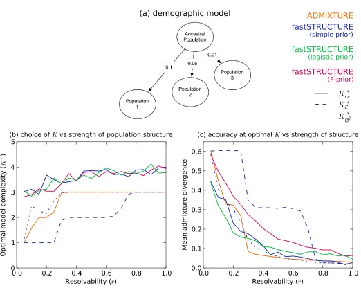
For theﬁrst group, the samples were drawn from a

three-population demographic model as shown in Figure 1A. The

edge weights correspond to the parameter F in the model

that quantiﬁes the genetic drift of each of the three current

populations from an ancestral population. We introduced

a scaling factor r2 [0, 1] that quantiﬁes the resolvability

of population structure underlying the samples. ScalingFby

rreduces the amount of drift of current populations from the

ancestral population; thus, structure is difﬁcult to resolve

whenris close to 0, while structure is easy to resolve when

(6)

generated 50 replicate data sets. The ancestral allele

fre-quenciespA_{for each data set were drawn from the frequency}

spectrum computed using the HGDP panel to simulate allele frequencies in natural populations. For each data set, the allele frequency at a given locus for each population was drawn from

a beta-distribution with meanpA_l and variancerFkpAlð12p

A lÞ,

and the admixture proportions for each sample were drawn from a symmetric Dirichlet distribution, namely Dirichlet

1 1013

, to

simulate small amounts of geneﬂow between the three

popu-lations. Finally, 10% of the samples in each data set, randomly selected, were assigned to one of the three populations with zero admixture.

For the second group, the samples were drawn from

a star-shaped demographic model withKtpopulations. Each

population was assumed to have equal drift from an

ances-tral population, with theFparameterﬁxed at either 0.01 to

simulate weak structure or 0.04 to simulate strong structure. The ancestral allele frequencies were simulated similar to

the ﬁrst group and 50 replicate data sets were generated

for this group for each value ofKt2{1,. . ., 5}. We executed

ADMIXTURE and fastSTRUCTURE for each data set with

various choices of model complexity: for data sets in theﬁrst

group, model complexityK2{1,. . ., 5}, and for those in the

second groupK2{1,. . ., 8}. We executed ADMIXTURE with

default parameter settings; with these settings the algorithm

terminates when the increase in log likelihood is,1024and

computes prediction error usingﬁvefold cross-validation.

fast-STRUCTURE was executed with a convergence criterion of change in the per-genotype log-marginal likelihood lower

boundjDEj,1028. We held out 20 random disjoint

geno-type sets, each containing 1% of entries in the genogeno-type matrix and used the mean and standard error of the deviance residuals for these held-out entries as an estimate of the pre-diction error.

For each group of simulated data sets, we illustrate a comparison of the performance of ADMIXTURE and fast-STRUCTURE with the simple and the logistic prior. When

structure was easy to resolve, both theF-prior and the logistic

prior returned similar results; however, the logistic prior returned more accurate ancestry estimates when structure

was difﬁcult to resolve. Plots including results using theF-prior

are shown in Supporting Information, Figure S1, Figure S2,

and Figure S3. Since ADMIXTURE uses held-out deviance

residuals to choose model complexity, we demonstrate the results of the two algorithms, each using deviance residuals

to chooseK, using solid lines in Figure 1 and Figure 2.

Addi-tionally, in theseﬁgures, we also illustrate the performance of

fastSTRUCTURE, when using the two alternative metrics to choose model complexity, using blue lines.

Choice of K

One question that arises when applying admixture models in practice is how to select the model complexity, or number of

populations,K. It is important to note that in practice there

will generally be no“true”value ofK, because samples from

real populations will never conform exactly to the

assump-tions of the model. Further, inferred values of K could be

inﬂuenced by sampling ascertainment schemes (Engelhardt

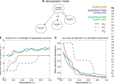
Figure 1 Accuracy of different algorithms as a function of resolv-ability of population structure. (A) Demographic model underlying the three populations represented in the simulated data sets. The edge weights quantify the amount of drift from the ancestral popula-tion. (B and C) Resolvability is a scalar by which the population-speciﬁc drifts in the demographic model are multiplied, with higher values of resolvability correspond-ing to stronger structure. (B) Com-pares the optimal model complexity given the data, averaged over 50 replicates, inferred by ADMIXTURE

ðK*

cvÞ, fastSTRUCTURE with simple

prior ðK_cv;* _K*

E;K∅*CÞ, and fast-STRUCTURE with logistic prior

ðK*

cvÞ. (C) Compares the accuracy

(7)

and Stephens 2010) (imagine sampling fromg distinct

loca-tions in a continuous habitat exhibiting isolation by distance—

any automated approach to selectKwill be inﬂuenced byg),

and by the number of typed loci (as more loci are typed, more

subtle structure can be picked up, and inferred values ofKmay

increase). Nonetheless, it can be helpful to have automated heuristic rules to help guide the analyst in making the

appro-priate choice forK, even if the resulting inferences need to be

carefully interpreted within the context of prior knowledge about the data and sampling scheme. Therefore, we here used

simulation to assess several different heuristics for selectingK.

The manual of the ADMIXTURE code proposes choosing model complexity that minimizes the prediction error on held-out data estimated using the mean deviance residuals reported

by the algorithmðK_cvÞ* _{. In Figure 1B, using the}_ﬁ_{rst group of}

simulations, we compare the value of K*

cv, averaged over 50

replicate data sets, between the two algorithms as a function of the resolvability of population structure in the data. We ob-serve that while deviance residuals estimated by ADMIXTURE robustly identify an appropriate model complexity, the value of

Kidentiﬁed using deviance residuals computed using the

var-iational parameters from fastSTRUCTURE appear to

overesti-mate the value ofKunderlying the data. However, on closer

inspection, we observe that the difference in prediction errors

between large values ofKare statistically insigniﬁcant (Figure

3, middle). This suggests the following heuristic: select the lowest model complexity above which prediction errors do

not vary signiﬁcantly.

Alternatively, for fastSTRUCTURE with the simple prior, we propose two additional metrics for choosing model

complexity: (1)K*

E, value ofKthat maximizes the LLBO of

the entire data set, and (2) K*

∅C, the limiting value, as K

increases, of the smallest number of model components that accounts for almost all of the ancestry in the sample. In

Figure 1B, we observe that K*

E has the attractive property

of robustly identifying strong structure underlying the data,

whileK*

∅C identiﬁes additional model components needed to

explain weak structure in the data, with a slight upward bias in complexity when the underlying structure is extremely

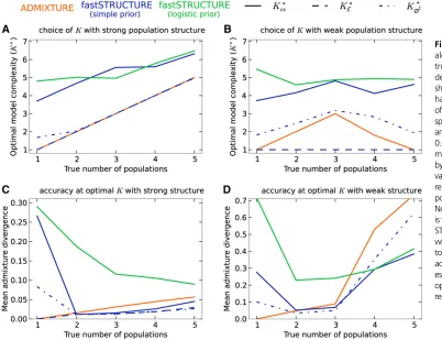
difﬁcult to resolve. For the second group of simulations,

similar to results observed for theﬁrst group, when

popula-tion structure is easy to resolve, ADMIXTURE robustly

iden-tiﬁes the correct value ofK(shown in Figure 2A). However,

for similar reasons as before, the use of prediction error with fastSTRUCTURE tends to systematically overestimate the

number of populations underlying the data. In contrast, K*

E

andK*

∅C match exactly to the trueKwhen population

struc-ture is strong. When the underlying population strucstruc-ture is

very weak,K*

E is a severe underestimate of the trueKwhile

K*

∅C slightly overestimates the value ofK. Surprisingly, K

*

cv

estimated using ADMIXTURE andK*

∅C estimated using

fast-STRUCTURE tend to underestimate the number of

popula-tions when the true number of populapopula-tions Kt is large, as

shown in Figure 2B.

For a new data set, we suggest executing fastSTRUCTURE

for multiple values of Kand estimating ðK*

E;K_∅*CÞ to obtain

(8)

a reasonable range of values for the number of populations that would explain structure in the data, under the given model. To look for subtle structure in the data, we suggest executing fastSTRUCTURE with the logistic prior with values for values of

Ksimilar to those identiﬁed by using the simple prior.

Accuracy of ancestry proportions

We evaluated the accuracy of the algorithms by comparing the divergence between the true admixture proportions and the estimated admixture proportions at the optimal model complexity computed using the above metrics for each data set. In Figure 1C, we plot the mean divergence between the true and estimated admixture proportions, over multiple replicates, as a function of resolvability. We observe that the admixture proportions estimated by fastSTRUCTURE

atK*

Ehave high divergence; however, this is a result of LLBO

being too conservative in identifying K. At K¼K*

cv and

K¼K*

∅C, fastSTRUCTURE estimates admixture proportions

with accuracies comparable to, and sometimes better than, ADMIXTURE even when the underlying population struc-ture is rather weak. Furthermore, the held-out prediction deviances computed using posterior estimates from variational algorithms are consistently smaller than those estimated by

ADMIXTURE (see Figure S3) demonstrating the improved

accuracy of variational Bayesian inference schemes over maximum-likelihood methods. Similarly, for the second group of simulated data sets, we observe in Figure 2, C and D, that the accuracy of variational algorithms tends to be comparable to or better than that of ADMIXTURE, particularly when

structure is difﬁcult to resolve. When structure is easy to

re-solve, the increased divergence estimates of fastSTRUCTURE with the logistic prior result from the upward bias in the

estimate ofK*

cv; this can be improved by using cross-validation

more carefully in choosing model complexity.

Visualizing ancestry estimates

Having demonstrated the performance of fastSTRUCTURE on multiple simulated data sets, we now illustrate the performance characteristics and parameter estimates using

two speciﬁc data sets (selected from the ﬁrst group of

simulated data sets), one with strong population structure

(r= 1) and one with weak structure (r= 0.5). In addition

to these algorithms, we executed STRUCTURE for these two data sets using the model of independent allele frequencies to directly compare with the results of fastSTRUCTURE. For

each data set, a was kept ﬁxed to 1

K for all populations,

(9)

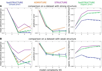
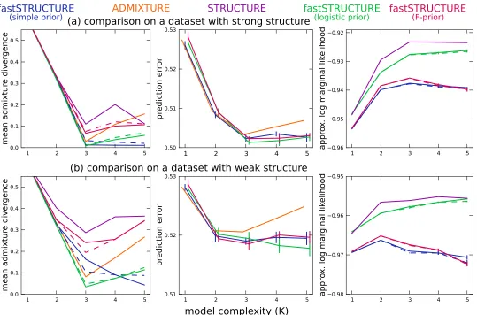
similar to the prior used for fastSTRUCTURE, and each run consisted of 50,000 burn-in steps and 50,000 MCMC steps. In Figure 3, we illustrate the divergence of admixture estimates and the prediction error on held-out data each as a function of

K. For all choices ofKgreater than or equal to the true value,

the accuracy of fastSTRUCTURE, measured using both ad-mixture divergence and prediction error, is generally compa-rable to or better than that of ADMIXTURE and STRUCTURE, even when the underlying population structure is rather weak. In Figure 3, right, we plot the approximate marginal likelihood of the data, reported by STRUCTURE, and the optimal LLBO, computed by fastSTRUCTURE, each as a function of

K. We note that the looseness of the bound between

STRUC-TURE and fastSTRUCSTRUC-TURE can make the LLBO a less reliable measure to choose model complexity than the approximate marginal likelihood reported by STRUCTURE, particularly

when the size of the data set is not sufﬁcient to resolve the

underlying population structure.

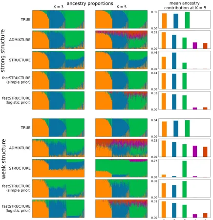
Figure 4 illustrates the admixture proportions estimated by the different algorithms on both data sets at two values of

K, using Distruct plots (Rosenberg 2004). For the larger

choice of model complexity, we observe that fastSTRUCTURE with the simple prior uses only those model components that are necessary to explain the data, allowing for automatic

(10)

inference of model complexity (Mackay 2003). To better il-lustrate this property of unsupervised Bayesian inference methods, Figure 4, right, shows the mean contribution of ancestry from each model component to samples in the data set. While ADMIXTURE uses all components of the model to

ﬁt the data, STRUCTURE and fastSTRUCTURE assign

negli-gible posterior mass to model components that are not re-quired to capture structure in the data. The number of

nonempty model componentsðK_∅CÞ automatically identiﬁes

the model complexity required to explain the data; the

opti-mal model complexityK*

∅C is then the mode of all values of

K_∅C computed for different choices ofK. While both

STRUC-TURE and fastSTRUCSTRUC-TURE tend to use only those model components necessary to explain the data, fastSTRUCTURE is slightly more aggressive in removing model components that seem unnecessary, leading to slightly improved results for fastSTRUCTURE compared to STRUCTURE in Equation 4, when there is strong structure in the data set. This property of fastSTRUCTURE seems useful in identifying global patterns

of structure in a data set (e.g., the populations represented in

a set of samples); however, it can be an important drawback if

one is interested in detecting weak signatures of gene ﬂow

from a population to a speciﬁc sample in a given data set.

When population structure is difﬁcult to resolve, imposing

a logistic prior and estimating its parameters using the data are likely to increase the power to detect weak structure. However, estimation of the hierarchical prior parameters by maximizing the approximate marginal likelihood also makes the model

susceptible to overﬁtting by encouraging a small set of samples

to be randomly, and often conﬁdently, assigned to unnecessary

components of the model. To correct for this, when using the logistic prior, we suggest estimating the variational parameters with multiple random restarts and using the mean of the

parameters corresponding to the topﬁve values of LLBO. To

ensure consistent population labels when computing the mean, we permuted the labels for each set of variational

parameter estimates toﬁnd the permutation with the lowest

pairwise Jensen–Shannon divergence between admixture

pro-portions among pairs of restarts. Admixture estimates com-puted using this scheme show improved robustness against

overﬁtting, as illustrated in Figure 4. Moreover, the pairwise

Jensen–Shannon divergence between admixture proportions

among all restarts of the variational algorithms can also be used as a measure of the robustness of their results and as

a signature of how strongly they overﬁt the data.

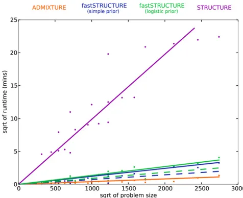
Runtime performance

A key advantage of variational Bayesian inference algo-rithms compared to inference algoalgo-rithms based on sampling is the dramatic improvement in time complexity of the algorithm. To evaluate the runtimes of the different learning

algorithms, we generated from the F-model data sets with

sample sizesN2{200, 600} and numbers of lociL2{500,

2500}, each having three populations withr= 1. The time

complexity of each of the above algorithms is linear in the

number of samples, loci, and populations, i.e., O(NLK); in

comparison, the time complexity of principal components analysis is quadratic in the number of samples and linear in the number of loci. In Figure 5, the mean runtime of the different algorithms is shown as a function of problem size

deﬁned as N 3 L 3 K. The added complexity of the cost

function being optimized in fastSTRUCTURE increases its runtime when compared to ADMIXTURE. However, fast-STRUCTURE is about 2 orders of magnitude faster than STRUCTURE, making it suitable for large data sets with hun-dreds of thousands of genetic variants. For example, using a data set with 1000 samples genotyped at 500,000 loci with

K= 10, each iteration of our current Python implementation

of fastSTRUCTURE with the simple prior takes about 11 min,

while each iteration of ADMIXTURE takes 16 min. Since

one would usually like to estimate the variational parameters

for multiple values ofKfor a new data set, a faster algorithm

that gives an approximate estimate of ancestry proportions in the sample would be of much utility, particularly to guide an

appropriate choice of K. We observe in our simulations that

a weaker convergence criterion ofjDEj,1026gives us

com-parably accurate results with much shorter run times, illus-trated by the dashed lines in Figure 3 and Figure 5. Based on these observations, we suggest executing multiple random restarts of the algorithm with a weak convergence criterion

of jDEj , 1025 to rapidly obtain reasonably accurate

esti-mates of the variational parameters, prediction errors, and ancestry contributions from relevant model components.

HGDP panel

We now compare the results of ADMIXTURE and fast-STRUCTURE on a large, well-studied data set of genotypes at single nucleotide polymorphisms (SNP) genotyped in the

HGDP (Li et al. 2008), in which 1048 individuals from

51 different populations were genotyped using Illumina’s

(11)

HumanHap650Y platform. We used the set of 938 “

unre-lated” individuals for the analysis in this article. For the

selected set of individuals, we removed SNPs that were

monomorphic, had missing genotypes in .5% of the

sam-ples, and failed the Hardy–Weinberg Equilibrium (HWE)

test at P , 0.05 cutoff. To test for violations from HWE,

we selected three population groups that have relatively little population structure (East Asia, Europe, Bantu Africa), constructed three large groups of individuals from these populations, and performed a test for HWE for each SNP

within each large group. The ﬁnal data set contained 938

samples with genotypes at 657,143 loci, with 0.1% of the entries in the genotype matrix missing. We executed AD-MIXTURE and fastSTRUCTURE using this data set with

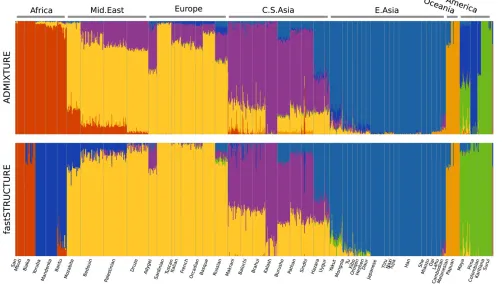
allowed model complexity K 2 {5, . . ., 15}. In Figure 6,

the ancestry proportions estimated by ADMIXTURE and

fast-STRUCTURE atK= 7 are shown; this value ofKwas chosen

to compare with results reported using the same data set

with FRAPPE (Liet al.2008). In contrast to results reported

using FRAPPE, we observe that both ADMIXTURE and fast-STRUCTURE identify the Mozabite, Bedouin, Palestinian, and Druze populations as very closely related to European

populations with some gene ﬂow from Central-Asian and

African populations; this result was robust over multiple random restarts of each algorithm. Since both ADMIXTURE and FRAPPE maximize the same likelihood function, the slight difference in results is likely due to differences in

the modes of the likelihood surface to which the two algo-rithms converge. A notable difference between ADMIXTURE and fastSTRUCTURE is in their choice of the seventh

pop-ulation—ADMIXTURE splits the Native American

popula-tions along a north–south divide while fastSTRUCTURE

splits the African populations into central African and south African population groups.

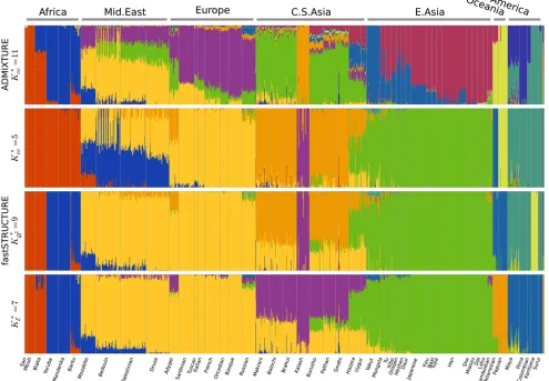
Interestingly, both algorithms strongly suggest the exis-tence of additional weak population structure underlying the data, as shown in Figure 7. ADMIXTURE, using

cross-validation, identiﬁes the optimal model complexity to be 11;

however, the deviance residuals appear to change very little

beyondK= 7, suggesting that the model components

iden-tiﬁed atK= 7 explain most of the structure underlying the

data. The results of the heuristics implemented in

fast-STRUCTURE are largely concordant, with K*

E¼7,K*_∅C¼9

and the lowest cross-validation error obtained atK*

cv¼10.

The admixture proportions estimated at the optimal choices of model complexity using the different metrics are shown in Figure 8. The admixture proportions estimated

atK= 7 andK= 9 are remarkably similar, with the Kalash

and Karitiana populations being assigned to their own

model components at K = 9. These results demonstrate

the ability of LLBO to identify strong structure underlying

the data and that ofK_∅C to identify additional weak structure

that explain variation in the data. At K= 10 (as identiﬁed

using cross-validation), we observe that only nine of the

(12)

model components are populated. However, the estimated admixture proportions differ crucially with all African popula-tions grouped together, the Melanesian and Papuan populapopula-tions each assigned to their own groups, and the Middle-Eastern populations represented as predominantly an admixture of Europeans and a Bedouin subpopulation with small amounts

of geneﬂow from Central-Asian populations.

The main contribution of this work is a fast, approximate inference algorithm for one simple admixture model for population structure, used in ADMIXTURE and STRUCTURE. While admixture may not be an exactly correct model for most population data sets, this model often gives key insights into the population structure underlying samples in a new data set and is useful in identifying global patterns of structure in the samples. Exploring model choice, by comparing the

goodness-of-ﬁt of different models that capture demographies of varying

complexity, is an important future direction.

Discussion

Our analyses on simulated and natural data sets demon-strate that fastSTRUCTURE estimates approximate posterior distributions on ancestry proportions 2 orders of magnitude faster than STRUCTURE, with ancestry estimates and pre-diction accuracies that are comparable to those of ADMIX-TURE. Posing the problem of inference in terms of an optimization problem allows us to draw on powerful tools in convex optimization and plays an important role in the gain in speed achieved by variational inference schemes, when compared to the Gibbs sampling scheme used in

STRUC-TURE. In addition, the ﬂexible logistic prior enables us to

resolve subtle structure underlying a data set. The consider-able improvement in runtime with comparconsider-able accuracies allows the application of these methods to large genotype data sets that are steadily becoming the norm in studies of population history, genetic association with disease, and conservation biology.

The choice of model complexity, or the number of

popula-tions required to explain structure in a data set, is a difﬁcult

problem associated with the inference of population structure. Unlike in maximum-likelihood estimation, the model parame-ters have been integrated out in variational inference schemes and optimizing the KL divergence in fastSTRUCTURE does not

run the risk of overﬁtting. The heuristic scores that we have

proposed to identify model complexity provide a robust and reasonable range for the number of populations underlying the data set, without the need for a time-consuming cross-validation scheme.

As in the original version of STRUCTURE, the model underlying fastSTRUCTURE does not explicitly account for linkage disequilibrium (LD) between genetic markers. While LD between genotype markers in the genotype data set will lead us to underestimate the variance of the approximate posterior distributions, the improved accuracy in predicting held-out genotypes for the HGDP data set demonstrates that

the underestimate due to unmodeled LD and the meanﬁeld

approximation is not too severe. Furthermore, not

account-ing for LD appropriately can lead to signiﬁcant biases in

local ancestry estimation, depending on the sample size and population haplotype frequencies. However, we believe global ancestry estimates are likely to incur very little bias due to unmodeled LD. One potential source of bias in global ancestry estimates is due to LD driven by segregating, chromosomal inversions. While genetic variants on inver-sions on the human genome and those of different model organisms are fairly well characterized and can be easily masked, it is important to identify and remove genetic variants that lie in inversions for nonmodel organisms, to avoid them from biasing global ancestry estimates. One heuristic approach to searching for such large blocks would be to compute a measure of differentiation for each locus between one population and the remaining populations, using the inferred variational posteriors on allele frequencies. Long stretches of the genome that have highly differentiated

(13)

genetic variants can then be removed before recomputing ancestry estimates.

In summary, we have presented a variational framework for fast, accurate inference of global ancestry of samples genotyped at a large number of genetic markers. For a new data set, we recommend executing our program, fastSTRUCTURE,

for multiple values ofKto obtain a reasonable range of values

for the appropriate model complexity required to explain structure in the data, as well as ancestry estimates at those model complexities. For improved ancestry estimates and to identify subtle structure, we recommend executing

fast-STRUCTURE with the logistic prior at values of K similar

to those identiﬁed when using the simple prior. Our program

is available for download athttp://pritchardlab.stanford.edu/

structure.html.

Acknowledgments

We thank Tim Flutre, Shyam Gopalakrishnan, and Ida Moltke for fruitful discussions on this project and the editor and two anonymous reviewers for their helpful comments

and suggestions. This work was funded by grants from the National Institutes of Health (HG007036,HG002585) and by the Howard Hughes Medical Institute.

Literature Cited

Alexander, D. H., J. Novembre, and K. Lange, 2009 Fast

model-based estimation of ancestry in unrelated individuals. Genome

Res. 19(9): 1655–1664.

Beal, M. J., 2003 Variational algorithms for approximate Bayesian

inference. Ph.D. Thesis, Gatsby Computational Neuroscience Unit, University College London, London.

Blei, D. M., A. Y. Ng, and M. I. Jordan, 2003 Latent dirichlet allocation.

J. Mach. Learn. Res. 3: 993–1022.

Carbonetto, P., and M. Stephens, 2012 Scalable variational

infer-ence for Bayesian variable selection in regression, and its

accu-racy in genetic association studies. Bayesian Anal. 7(1): 73–108.

Catchen, J., S. Bassham, T. Wilson, M. Currey, C. O’Brienet al.,

2013 The population structure and recent colonization history

of Oregon threespine stickleback determined using

restriction-site associated DNA-sequencing. Mol. Ecol. 22: 2864_–2883.

Engelhardt, B. E., and M. Stephens, 2010 Analysis of population

structure: a unifying framework and novel methods based on sparse factor analysis. PLoS Genet. 6(9): e1001117.

Figure 8 Ancestry proportions inferred by ADMIXTURE and fastSTRUCTURE (with the simple prior) at the optimal choice ofKidentiﬁed by relevant metrics for each algorithm. Notably, the admixture proportions atK¼K*

(14)

Falush, D., M. Stephens, and J. K. Pritchard, 2003 Inference of population structure using multilocus genotype data: linked loci

and correlated allele frequencies. Genetics 164: 1567–1587.

Hofman, J. M., and C. H. Wiggins, 2008 Bayesian approach to

network modularity. Phys. Rev. Lett. 100(25): 258701. Hubisz, M. J., D. Falush, M. Stephens, and J. K. Pritchard,

2009 Inferring weak population structure with the assistance

of sample group information. Mol. Ecol. Res. 9(5): 1322–1332.

Jordan, M. I., Z. Gharamani, T. S. Jaakkola, and L. K. Saul,

1999 An introduction to variational methods for graphical

models. Mach. Learn. 37(2): 183_–233.

Kadanoff, L. P., 2009 More is the same: phase transitions and

mean_ﬁeld theories. J. Stat. Phys. 137(5_–6): 777_–797.

Li, J. Z., D. M. Absher, H. Tang, A. M. Southwick, A. M. Castoet al.,

2008 Worldwide human relationships inferred from

genome-wide patterns of variation. Science 319(5866): 1100–1104.

Logsdon, B. A., G. E. Hoffman, and J. G. Mezey, 2010 A variational

Bayes algorithm for fast and accurate multiple locus genome-wide association analysis. BMC Bioinformatics 11(1): 58.

Mackay, D. J., 2003 Information theory, inference and learning

algorithms. Cambridge University Press, Cambridge, UK.

Novembre, J., and M. Stephens, 2008 Interpreting principal

com-ponent analyses of spatial population genetic variation. Nat.

Genet. 40(5): 646–649.

Patterson, N., A. L. Price, and D. Reich, 2006 Population structure

and eigenanalysis. PLoS Genet. 2(12): e190.

Pearse, D., and K. Crandall, 2004 Beyond FST: analysis of

popu-lation genetic data for conservation. Conserv. Genet. 5(5): 585–

602.

Pickrell, J. K., and J. K. Pritchard, 2012 Inference of population

splits and mixtures from genomewide allele frequency data. PLoS Genet. 8(11): e1002967.

Price, A. L., N. J. Patterson, R. M. Plenge, M. E. Weinblatt, N. A.

Shadicket al., 2006 Principal components analysis corrects for

stratiﬁcation in genomewide association studies. Nat. Genet. 38

(8): 904–909.

Pritchard, J. K., and P. Donnelly, 2001 Case-control studies of

association in structured or admixed populations. Theor. Popul.

Biol. 60(3): 227–237.

Pritchard, J. K., M. Stephens, and P. Donnelly, 2000 Inference of

population structure using multilocus genotype data. Genetics

155: 945–959.

Randi, E., 2008 Detecting hybridization between wild species and

their domesticated relatives. Mol. Ecol. 17(1): 285–293.

Raydan, M., and B. F. Svaiter, 2002 Relaxed steepest descent and

Cauchy_–Barzilai_–Borwein method. Comput. Optim. Appl. 21(2):

155_–167.

Reich, D., K. Thangaraj, N. Patterson, A. L. Price, and L. Singh,

2009 Reconstructing Indian population history. Nature 461

(7263): 489–494.

Rosenberg, N. A., 2004 DISTRUCT: a program for the graphical

display of population structure. Mol. Ecol. Notes 4(1): 137–138.

Rosenberg, N. A., J. K. Pritchard, J. L. Weber, H. M. Cann, K. K. Kidd

et al., 2002 Genetic structure of human populations. Science

298(5602): 2381–2385.

Sato, M. A., 2001 Online model selection based on the variational

Bayes. Neural Comput. 13(7): 1649–1681.

Tang, H., J. Peng, P. Wang, and N. J. Risch, 2005 Estimation of

individual admixture: analytical and study design

considera-tions. Genet. Epidemiol. 28(4): 289–301.

Teh, Y. W., D. Newman, and M. Welling, 2007 A collapsed

varia-tional Bayesian inference algorithm for latent Dirichlet allocation. Adv. Neural Inf. Process. Syst. 19: 1353.

Varadhan, R., and C. Roland, 2008 Simple and globally

conver-gent methods for accelerating the convergence of any EM

algo-rithm. Scand. J. Stat. 35(2): 335_–353.

(15)

Appendix A

Given the parametric forms for the variational distributions and a choice of prior for the fastSTRUCTURE model, the per-genotype LLBO is given as

E ¼_G1X

n;l

dðGnlÞ

( X

k

EZnlka

þEZbnlk

I½Gnl¼0E

logð12PÞlk

þI½Gnl¼2E½logPlk þE½logQnk

þI½Gnl¼1

X

k

EZa_nlkE½logPlk þE

Zb_nlkE½logð12PlkÞ

2ElogZ_nla2ElogZ_nlb

)

þX

l;k

logB

_~

Pulk;P~ v lk

Bðb;gÞ þ

b2~Pu_lkE½logPlk þ

g2P~v_lkE½logð12PlkÞ

þX n ( X k

ak2Qnk~

E½logQnk þlogGðakÞ2logG

_~

Qnk

)

þlogGQno~ 2logGðaoÞ; (A1)

whereE[] is the expectation taken with respect to the appropriate variational distribution, B() is the beta function,G() is

the gamma function, {a,b,g} are the hyperparameters in the model,d() is an indicator variable that takes the value of zero

if the genotype is missing, G is the number of observed entries in the genotype matrix,ao¼

P

kak, and Q~no¼

P

kQ~nk.

Maximizing this lower bound for each variational parameter, keeping the other parameters ﬁxed, gives us the following

update equations:

_~

Za;~Zb:

~

Zanlk}exp

n

Ca Gnl2c

_~

PulkþP~ v lk

þcQnk~ 2cQno~ o (A2)

~

Zbnlk}exp

n

Cb Gnl2c

~

PulkþP~ v lk

þcQnk~ 2cQno~ o; (A3)

where

Ca

Gnl¼I½Gnl¼0c

~

Pv_lk

þI½Gnl¼1c

~

Pu_lk

þI½Gnl¼2c

~

Pu_lk

(A4)

Cb

Gnl¼I½Gnl¼0c

~

Pvlk

þI½Gnl¼1c

~

Pvlk

þI½Gnl¼2c

~

Pulk

(A5)

~

Q:

~

Qnk¼akþ

X

l

dðGnlÞ

~

Za_nlkþ~Zb_nlk

(A6)

_~

Pu;~Pv:

~

Pu_lk¼bþX

n

I½Gnl¼1Z~ a

nlkþI½Gnl¼2

~

Za_nlkþ~Zb_nlk (A7)

~

Pvlk¼gþ

X

n

I½Gnl¼1~Z b

nlkþI½Gnl¼0

~

ZanlkþZ~ b nlk

: (A8)

In the above update equations,c() is the digamma function. When theF-prior is used, the LLBO and the update equations

remain exactly the same, after replacing bwith pA_lð½12Fk=FkÞ andg with ð12pA_lÞð½12Fk=FkÞ. In this case, the LLBO

is also maximized with respect to the hyperparameter F using the L-BFGS-B algorithm, a quasi-Newton code for

(16)

When the logistic prior is used, a straightforward maximization of the LLBO no longer gives us explicit update equations

for P~ulk andP~

v

lk. One alternative is to use a constrained optimization solver, like L-BFGS-B; however, the large number of

variational parameters to be optimized greatly increases the per-iteration computational cost of the inference algorithm.

Instead, we propose update equations forP~ulkand~P

v

lkto have a similar form as those obtained with the simple prior,

~

Pu_lk¼b_lkþX

n

I½Gnl¼1~Z a

nlkþI½Gnl¼2

~

Z_nlka þZ~_nlkb

(A9)

~

Pv_lk¼glkþ

X

n

I½Gnl¼1~Z b

nlkþI½Gnl¼0

~

Z_nlka þ~Z_nlkb

; (A10)

whereblkandglkimplicitly depend on~P

u lkand~P

v

lkas follows:

c9P~ulk

2c9P~ulkþP~ v lk

b_lk2c9P~ulkþP~ v lk

g_lk¼2lkc9

_~

Pulk

c~Pulk

2c~Pvlk

2m_l 21

2lkc$

_~

Pulk

2c9P~ulkþP~ v lk

b_lk

þc9

~

Pu_lk

2c9

~

Pu_lkþ~Pv_lk

glk¼lkc9

~

Pv_lk

c

~

Pu_lk

2c

~

Pv_lk

2ml

21

2lkc$

~

Pvlk

: (A11)

The optimal values for~Pulkand~P

v

lkcan be obtained by iterating between the two sets of equations to convergence. Thus, when

the logistic prior is used, the algorithm is implemented as a nested iterative scheme where for each update of all the

variational parameters, an iterative scheme computes the update forð~Pu_;~_Pv_Þ_{. Finally, the optimal value of the}

hyperpara-metermis obtained straightforwardly as

m_l¼X

k lk c ~

Pulk

2c

~

Pvlk

.X

k

lk (A12)

while the optimal lis computed using a constrained optimization solver.

Appendix B

Given the observed genotypesG, the probability of the unobserved genotypeGhid

nl for thenth sample at thelth locus is given as

pðGhid_nl jGÞ ¼

Z

pðGhid_nl jP;QÞpðP;QjGÞ dQ dP: (B1)

Replacing the posterior p(P,Q|G) with the optimal variational posterior distribution, we obtain

pðGhid_nl ¼0Þ

Z

pðGhid_nl ¼0jP;QÞqðPÞqðQÞ dQ dP (B2)

¼X

k;k9

Z

QnkQnk₉ð12PlkÞð12Plk₉ÞqðPÞqðQÞ dQ dP (B3)

¼X

k6¼k9

E½QnkQnk₉ð12E½PlkÞð12E½Plk₉Þ (B4)

þX

k¼k9

EQ2_nkE

h

ð12PlkÞ2

i

(B5)

pðGhidnl ¼1Þ

Z

(17)

¼2X

k;k9

Z

QnkQnk9Plk

12Plk9

qðPÞqðQÞ dQ dP (B7)

¼X

k6¼k9

EQnkQnk9E½P_lk12EP_lk9 (B8)

þX

k¼k9

EQ2_nkEhPlkð12PlkÞ

i

(B9)

pðGhid_nl ¼2Þ

Z

pðGhid_nl ¼2jP;QÞqðPÞqðQÞ dQ dP (B10)

¼X

k;k9

Z

QnkQnk9PlkP_lk9qðPÞqðQÞ dQ dP (B11)

¼X

k6¼k9

EQnkQnk9

E½PlkEPlk9

(B12)

þX

k¼k9

EQ2_nkEP2_lk; (B13)

where

EQnkQnk9¼

~

QnkQ~nk9

~

QnoðQno~ þ1Þ (B14)

EQ2nk

¼Q~nk

_~

Qnkþ1

~

QnoðQno~ þ1Þ (B15)

E½Plk ¼

~

Pu_lk

~

Pu_lkþ~Pv_lk (B16)

EP2_lk¼ ~P u lk

_~

Pu_lkþ1

_~

Pu_lkþ~Pv_lkP~u_lkþP~v_lkþ1 (B17)

E½Plkð12PlkÞ ¼

~

Pulk~P v lk

_~

PulkþP~ v lk

_~

Pulkþ~P v lkþ1

(B18)

Ehð12PlkÞ2

i

¼ P~

v lk

_~

Pvlkþ1

_~

PulkþP~ v lk

_~

Pulkþ~P v lkþ1

: (B19)

(B20)

(18)

GENETICS

Supporting Information

http://www.genetics.org/lookup/suppl/doi:10.1534/genetics.114.164350/-/DC1

fastSTRUCTURE: Variational Inference of Population

Structure in Large SNP Data Sets

Anil Raj, Matthew Stephens, and Jonathan K. Pritchard

(19)

0.0

0.2

0.4

0.6

0.8

1.0 Resolvability (

r

)

0

1

2

3

4

5 Op

tim

al

mo

de

l c

om

ple

xit

y (

K

∗

)

0.0

0.2

0.4

0.6

0.8

1.0 Resolvability (

r

)

0.0

0.1

0.2

0.3

0.4

0.5

0.6 Me

an

ad

mi

xtu

re

div

erg

en

ce

(a) demographic model

(b) choice of

K

vs strength of population structure

(c) accuracy at optimal

K

vs strength of structure

ADMIXTURE

fastSTRUCTURE

_{(simple prior)}

fastSTRUCTURE

_{(logistic prior)}

fastSTRUCTURE

_(F-prior)

cv), fastSTRUCTURE with

simple prior (

K

cv∗

, K

∗ E

0.1 0.2 0.3 0.4 0.5

me

an

ad

mi

xtu

re

div

erg

en

ce

1

2

3

4

5

0.50 0.51 0.52 0.53

pre

dic

tio

n e

rro

r

1 2 3 4 5

−0.96 −0.95 −0.94 −0.93 −0.92

ap

pro

x.

log

m

arg

ina

l li

ke

lih

oo

d

1 2 3 4 5

0.0 0.1 0.2 0.3 0.4 0.5

me

an

ad

mi

xtu

re

div

erg

en

ce

1 2 3 4 5

0.51 0.52 0.53

pre

dic

tio

n e

rro

r

1 2 3 4 5

−0.98 −0.97 −0.96 −0.95