Extending Scojo-PECT by migration based on application level checkpointing

University of Windsor University of Windsor

Scholarship at UWindsor

Scholarship at UWindsor

Electronic Theses and Dissertations Theses, Dissertations, and Major Papers

2009

Extending Scojo-PECT by migration based on application level

Extending Scojo-PECT by migration based on application level

checkpointing

checkpointing

Jiaying Shi

University of Windsor

Follow this and additional works at: https://scholar.uwindsor.ca/etd

Recommended Citation Recommended Citation

Shi, Jiaying, "Extending Scojo-PECT by migration based on application level checkpointing" (2009). Electronic Theses and Dissertations. 7923.

https://scholar.uwindsor.ca/etd/7923

This online database contains the full-text of PhD dissertations and Masters’ theses of University of Windsor students from 1954 forward. These documents are made available for personal study and research purposes only, in accordance with the Canadian Copyright Act and the Creative Commons license—CC BY-NC-ND (Attribution, Non-Commercial, No Derivative Works). Under this license, works must always be attributed to the copyright holder (original author), cannot be used for any commercial purposes, and may not be altered. Any other use would require the permission of the copyright holder. Students may inquire about withdrawing their dissertation and/or thesis from this database. For additional inquiries, please contact the repository administrator via email

Extending Scojo-PECT by migration based on

application level checkpointing

By

Jiaying Shi

A Thesis

Submitted to the Faculty of Graduate Studies through the School of Computer Science in Partial Fulfillment of the Requirements for

the Degree of Master of Science at the University of Windsor

Windsor, Ontario, Canada 2009

1*1

Published Heritage Branch

395 Wellington Street OttawaONK1A0N4 Canada

Bibliotheque et Archives Canada

Direction du

Patrimoine de I'edition

395, rue Wellington OttawaONK1A0N4 Canada

Your file Votre reference ISBN: 978-0-494-57636-6 Our file Notre reference ISBN: 978-0-494-57636-6

NOTICE: AVIS:

The author has granted a

non-exclusive license allowing Library and Archives Canada to reproduce,

publish, archive, preserve, conserve, communicate to the public by

telecommunication or on the Internet, loan, distribute and sell theses

worldwide, for commercial or non-commercial purposes, in microform, paper, electronic and/or any other formats.

L'auteur a accorde une licence non exclusive permettant a la Bibliotheque et Archives Canada de reproduire, publier, archiver, sauvegarder, conserver, transmettre au public par telecommunication ou par I'lnternet, preter, distribuer et vendre des theses partout dans le monde, a des fins commerciales ou autres, sur support microforme, papier, electronique et/ou autres formats.

The author retains copyright ownership and moral rights in this thesis. Neither the thesis nor substantial extracts from it may be printed or otherwise reproduced without the author's permission.

L'auteur conserve la propriete du droit d'auteur et des droits moraux qui protege cette these. Ni la these ni des extraits substantiels de celle-ci ne doivent etre imprimes ou autrement

reproduits sans son autorisation.

In compliance with the Canadian Privacy Act some supporting forms may have been removed from this thesis.

Conformement a la loi canadienne sur la protection de la vie privee, quelques

formulaires secondaires ont ete enleves de cette these.

While these forms may be included in the document page count, their removal does not represent any loss of content from the thesis.

Bien que ces formulaires aient inclus dans la pagination, il n'y aura aucun contenu manquant.

1+1

Author's Declaration of Originality

I hereby certify that I am the sole author of this thesis and that no part of this thesis has

been published or submitted for publication.

I certify that, to the best of my knowledge, my thesis does not infringe upon anyone's

copyright nor violate any proprietary rights and that any ideas, techniques, quotations, or

any other material from the work of other people included in my thesis, published or

otherwise, are fully acknowledged in accordance with the standard referencing practices.

Furthermore, to the extent that I have included copyrighted material that surpasses the

bounds of fair dealing within the meaning of the Canada Copyright Act, I certify that 1

have obtained a written permission from the copyright owner(s) to include such

material(s) in my thesis and have included copies of such copyright clearances to my

appendix.

I declare that this is a true copy of my thesis, including any final revisions, as approved

by my thesis committee and the Graduate Studies office, and that this thesis has not been

Abstract

In parallel computing, jobs have different runtimes and required computation resources.

With runtimes correlated with resources, scheduling these jobs would be a packing

problem getting the utilization and total execution time varies. Sometimes, resources are

idle while jobs are preempted or have resource conflict with no chance to take use of

them. This greatly wastes system resource at certain degree.

Here we propose an approach which takes periodic checkpoints of running jobs with the

chance to take advantage of migration to optimize our scheduler during long term

scheduling. We improve our original Scojo-PECT preemptive scheduler which does not

have checkpoint support before. We evaluate the gained execution time minus overhead

To my wife, Xiaoguang Li

Acknowledgements

I would like to take this opportunity to express my sincere gratitude to my supervisor Dr.

Angela C. Sodan. Without her extensive guidance and constant encouragement, I could

not finish this thesis. I would also like to thank all committee members, Dr. Roberto

Muscedere, Dr. Xiaobu Yuan and Dr. Dan Wu for their valuable time and comments.

My special thanks go to my wife, Xiaoguang Li, for her support and good advices during

the two and half years' graduate study.

I would like to thank Lichun Zhu for his great work on modifying and debugging

programs; Peiyu Cai for his idea and help on assuming algorithm; Xijie Zeng, Wei Jin

and Xiaorong Cao for the happy experience during the time I worked with them.

Last, but not least, I would like to thank all of my friends for all the help and support

Table of Contents

Author's Declaration of Originality ..iii

Abstract iv

Dedication v

Acknowledgements vi

List of Tables ix

List of Figures x

1. Introduction 1

2. .Background Issues: 5

3. Scojo-PECT 8

3.1 Scojo-PECT Preemptive Scheduler 8

3.2 Core Scheduling Algorithm 9

4. Extended Job Scheduling Algorithm 11

4.1 Assumption, Motivation, Scheduling Objective 11

4.2 Cost Model 12

4.2.1 Trend of Checkpoint File Sizes 12

4.2.2 Interval Setting 19

4.3 Checkpointing Scheme by Migration with Checkpointing at Application Level 22

5. Experiment and Result Analysis

5.1 Experiment Environment Setup 30

5.1.1 Workload Modeling 30

5.1.2 Evaluation Plan 31

5.2 Experiment of Results 33

5.3 Result Analysis 39

6. Conclusion and Future Work 41

6.1 Conclusion 41

6.2 Future Work 41

Reference 43

Appendix 46

List of Tables

Table 1. Relation Chart of Application & System Level Checkpoint 13

Table 2. Scheduler Parameters 31

List of Figures

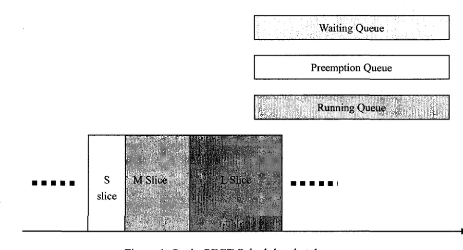
Figure 1. Scojo-PECT Scheduler sketch map 10

Figure 2 Chart of relation between application and system file sizes 14

Figure 3. Probability density function & Cumulative distribution function 15

Figure 4. Relation of reduction of file size in ISING and SOR applications 17

Figure 5. The (PDF) probability density function and (CDF) cumulative distribution

function of gamma distribution 18

Figure 6. MTBF chart under different reliability level 20

Figure 7. Probability density function of normal distribution 21

Figure 8 Job initialization stage 23

Figure 9 Migration stage 26

Figure 10 Migration & Backfill 28

Figure 11 Relative Response Time for long and medium jobs at seed 71 34

Figure 12 Relative Response Time for long and medium jobs at seed 31 35

Figure 13 Relative Response Time for long and medium jobs at seed 7 36

Figure 14 Relative Response Time for long and medium jobs at seed 23 37

Figure 15 Relative Response Time for long and medium jobs at seed 13 38

1. Introduction _

In high performance computing area, a job has one or more processes, like serial job and

parallel job. People cared about how to schedule the jobs that would bring more benefit.

There are three metrics to evaluate a schedule strategy. At users' view, response time

defines how fast the job has been processed. It is the time period between job submission

and termination. Usually we use average response time instead of each individual one. As

some situations did exist when average response time got good result, while several

specific jobs were severely delayed. So, another metric fairness would be counted in. It is

the factor to check whether the job is fairly or unfairly treated. It sets up a threshold to

compare a job's response time and its estimated response time as it's been submitted. At

systems' view, utilization defines how efficient the resources have been taken advantage

of. It could be counted as a relation between used and total resource during a time scale.

Better utilization would lead to shorter response time but not guarantee in every case.

Thus, sometimes there is a tradeoff between response time and utilization.

There are two basic types of job scheduling approaches: time sharing and space sharing.

For time sharing, multiple jobs are allocated to run on the same set of processors.

Multiple processes share using a processor with time slices. The advantage of time

sharing is that jobs can start to run sooner (maybe result as a shorter response time).

Regarding space sharing, processors are divided into groups and each group exclusively

suspended. Space sharing is easy to implement without any context switch overhead.

Unfortunately, inefficient packing schemes usually generate fragmentations. Some

scheduling methods are proposed to improve the performance of time and space sharing,

e.g. backfilling, by which a job is scheduled to run out of its original FCFS (First Come

First Serve) order to fill the "holes".

Checkpointing mechanism is a term we often used in database and high-performance

computing area. It keeps the current program's computation state into stable storages for

the purpose of recovery once occur failure and get restart with minimum loss of

computing work. We extended the original scheduler to take use of checkpoint

mechanism not for fault tolerance but for the resource flexibility by storing the

computation state periodically. As the original scheduler does not support the checkpoint

and it only does preemption (suspend jobs when slice ends and resume on the same

resource in its own type slice), it greatly restricts the usage of computation resource even

if there is free resource.

A checkpoint of a single process contains the processor's address space and states of its

registers. And a global state is required in additional in multi-processor and distributed

systems. It has the information to describe the relationship between checkpoints of each

processor. To restart from a checkpoint, it just needs to initialize the address space from

Two basic types of checkpointing schemes are full checkpointing and incremental

checkpointing. With full checkpointing, the system just saves the whole image of current

process state into stable storage. And incremental checkpointing, it maintains a list of all

the dirty pages of memory which has been modified during the computation since the last

checkpoint. When reaching the checkpoint, only those pages on the list will be stored

since the remaining pages are just read only variables. The latter approach would save

larger space in checkpoint file size and thus reduce the checkpoint overhead greatly.

There is another classification method based on platforms, several major categories of

checkpointing are: Hardware level, additional hardware incorporates with processor to

save state; System/Kernel level, operation system will be responsible for taking

checkpoint; Application level, the checkpoint code is directly inserted into application by

programmer or preprocessor. Application level checkpoint (ALC): for this definition, it is

a checkpointing technique in application level. It highly depends on programmer who is

required to have sufficient knowledge on specific applications. In the abstraction level, it

selects relevant core of data in order to reduce the amount of checkpoint file size and

achieve more efficient operation by pre-compiler, which we will discuss in background

issue for more detail.

In our thesis, we extended original scheduler by adding application level checkpoint.

in utilization and average relative response time.

The rest of the thesis is organized as follows. Background issues are discussed in Chapter

2. Chapter 3 introduces original Scojo-PECT. And extended job scheduling algorithm is

described in detail in Chapter 4. Chapter 5 presents the simulation, experiments and

results analysis. Finally, the conclusion of the thesis is made in Chapter 6 and we discuss

2. Background Issues:

Job scheduling in parallel computing area has been studied for a long period. Around the

scheduling approaches, there is generally not only the time sharing and the space sharing,

but also other mechanisms involved such as preemption and backfill. However, these

approaches could partially solve the fragmentation created during arranging jobs phase

and make better use of idle resource avoiding making nodes unfairly working(the

situation some nodes running busy, some keep idle).

There is now another option to improve the performance of total job scheduling using

migration based on checkpointing, which we discussed above. One type is system level

checkpointing, and the other is application level checkpointing. For system level

checkpointing, University of Wisconsin introduced Condor system [14] which provides

important features that: Source code does not need to be modified to take advantage of

these benefits. Code that can be re-linked with the Condor libraries then the jobs can

produce checkpoints and they can perform remote system calls [14], and Lawrence

Berkeley National Laboratory introduced BLCR (Berkeley Lab Checkpoint/Restart) [16],

a system-level checkpoint/restart implementation for Linux clusters that targets the space

of typical High Performance Computing applications, including MPI. As a kernel module,

it has a "callback" interface to allow any library or application code to cooperate in the

For application level checkpointing, Cornell University introduced C3 (Cornell

Checkpoint Compiler) [15] system, it executes almost all source code and instruments

them to perform application level state saving by insert a potential checkpoint at locations

in the application where checkpoints might be taken. And the pre-compiler co-work with

the native compiler of hardware platform to interpret the calls from the instrument

application.

As those two kinds of checkpointing mechanisms present, which one would be better for

high performance computation. What is the exact difference between them?

The differences between System level vs. Application level checkpointing techniques:

One is the checkpoint file size. As we know, the system level checkpointing approach

barely has the knowledge of what application it is. It just stores the whole image of

process at the time it takes the checkpoint. For application level checkpointing approach,

it is been assumed the programmer has sufficient knowledge on applications and could

tell what kind of variables are dead, which part of image could be compressed. In this

manner, the size of checkpoint file get smaller compare to system one. In [15], authors

made comparison between C3 and Condor, used five kinds of applications for testing, it

proved ALC could have smaller size compare to SLC, though results varies.

level, the operation system will handle the checkpoint and decide when to generate a

checkpoint, what is more, that kind of checkpoint in system level could be done at

arbitrary time as the processes has been preempted with no risk of lacking records. The

application level, the application at the beginning based on its own code will have no idea

when and how to do the checkpoint operation. So inserting the intervals for application

level checkpointing would be better choice for the simulation. In [1][2][3], the authors

studied on determining the optimal interval for setting checkpoints in application and

made proof. [2][3], are continuous study and the authors in latter made great efforts

modifying the formula to let it suits more cases and made more accurate to predict the

interval.(the former failed to make prediction on small size of checkpoint file) And in [1],

author tried to verify the impacts over the system overall quality of interval setting

through many aspects, as they put interval as adjustable parameter and they also pointed

out the optimal checkpoint intervals heavily depend on some system parameters, such as

the time to place a checkpoint, the time to recover from a fault, the fault arrival rate,

which has the similarity with [2] [3]. And for this reason, we decided to take advantage of

their existing parameter and formula to make it suitable to our research.

As the checkpointing mechanism usually is applied in HPC (High Performance

Computing) field for the purpose of fault tolerance, we imported the idea into our work as

a solution to let the application have more flexibility choosing free computation resource

3. Scojo-PECT

The extending work is all based on the Scojo-PECT. In this chapter, we are going to

discuss the detailed original scheduler including how it works, what kind of scheduling

techniques have been adopted and also some priorities of jobs.

3.1 Scojo-PECT Preemptive Scheduler

Scojo-PECT [8] is a job scheduler framework. Scojo-PECT provides coarse grain time

slices to avoid the excessive waiting time when jobs getting access to their resource. All

running jobs are preempted and divided into three types (short, medium, long) based on

their runtimes. This could make the preemption in the disk affordable. They are

scheduled in different time slices of their own types.

Scojo-PECT does not require checkpointing [10] support and therefore impose the

constraint that preemption jobs without checkpoint could just restart on the same resource

instead of migrating to different resources. One slice time of each type was scheduler per

time interval which was set based on the resource time share which is predefined.

Resource shares [9] can be defined based on specific job mixes, administrator's policies.

E.g. it can be set different for different times during the day.

Scojo-PECT can either use EASY or conservative backfilling. Backfilling is an approach

means jobs could be move ahead by not delay the first waiting job. Conservative

backfilling [10] requires none jobs in queue to be delayed compare to their schedule

position upon submission. Within the scheduler, the job will not dynamically change and

jobs per type were typically scheduled in FCFS order with backfilling applied.

Scojo-PECT also provides safe non-type backfilling [8] because the manual division of

job into several types may generate fragmentations since job runtimes and job sizes are

correlated. Non-type backfilling means preempted or waiting jobs of different slices can

be backfill to a slice if they do not delay any jobs of the slice type or their own types.

Scojo-PECT implemented an event-driven simulator to have it co-work with scheduler.

The event-based simulator defines four kinds of events with job submission and

termination mean new job come into waiting queue and job finish running and release the

occupied resources. Slice begin events describe new time slice starts and specific jobs

resumed/scheduled to run and slice end events means one slice run out of its time share

and all running jobs are preempted.

3.2 Core Scheduling Algorithm

The detailed original algorithm of Scojo-PECT [8] is:

At first, at the end of slice, jobs were preempted at the end of corresponding time slice

Second, scheduler attempts to schedule jobs of slice type from waiting queue which first

fit the free resource;

Then, scheduler tries to backfill (EASY or Conservative) of slice type;

Last, scheduler will try to non-type backfill (e.g. using the medium and long type job in

their waiting queue to backfill the fragmentation left in small job type slice).

Waiting Queue

Preemption Queue

Running Queue

4. Extended Job Scheduling Algorithm

In this chapter, we are going to discuss how we extended the original scheduler. We start

talking about the motivation and objective. And we explain the cost model (interval

setting, overhead distribution calculation) we have applied in our experiment in detail. At

last, we will discuss the extended job scheduling algorithm such as how it works, what

extra benefit it could get compared to original scheduler. After that, we will analyze the

potential benefit of a simple case by adopting our extending job scheduling algorithm.

4.1 Assumption, Motivation, Scheduling Objective

The extending of applying application level checkpoint is based on the following

assumptions:

1. We introduce checkpoint in our simulator as an approach for flexibly using free

resource, not for the aim of failure recovery

2. All the jobs randomly generated by Lublin-Feitelson model are independent

As we discussed the original Scojo-PECT, it has feature like preemption while it will

restrict scheduler to make decision on using idle resources even there are available. And

originally the Scojo-PECT did not have checkpoint support, for this reason, we imported

checkpoint/migration mechanism to let the scheduler to better utilize resource much

The objective of the scheduler one is to get better average response time based on

different workload model. The response time means the time cost between jobs been

submit and return back. It generally represents the efficiency of scheduler processing

operation. Another is to find out the relation between the average response time and

relative factors like average job size, randomly job generation and also job type ratio.

4.2 Cost Model

As we discussed in background issue, there are two major differences between system

and application level checkpoint. One is the file size, and the other checkpoint time. For

the first, we involved the gamma distribution [11] and we will discuss it in detail at below,

and the latter, we borrowed their formula for setting up optimal intervals for application

level checkpoint [3].

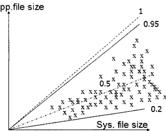
4.2.1 Trend of Checkpoint File Sizes

The background of this function is our investigation of other peoples' experiment results

between system level and application level checkpoint sizes using different categories of

program. The most common situation is the application level will reduce the full size of

checkpoint files in system level to the average of 50%, which in another way means

nearly half space of checkpoint file could be saved by applying the modification in

application level [5].While, there are still some specific application required more on the

levels will be less, vice versa. Two extreme cases are the application level checkpoint

files nearly be the same as the system level one; and the application level checkpoint file

shrink tremendously and close to 20%, shows in Table 1. So we manually set the statistic

bound ranges from 20% to 95% of the full size of system level checkpoint file [5][6].

With the trend, as it closes to the low bound 20%, the probability of density is higher,

which means there is much higher possibility to reduce the checkpoint file size for at

least 20%, and to the other side, high bound 95%, the probability of density is almost

none means there is little chance for application level checkpoint reduce the file size for

95%. Applications ISLNG 256 ISING512 ISING768 ISING 1024 ISING urn ISING 1536 ISING 1792 SOR25C 80RS12 SOR 768 SOR1024 SOR1280 GAUSS 512 GAUSS 1024 ASP 512 ASP 1024 2*BODY40» System-Level Checkpoints 3176 3962 5268 7082 9408 12251 15601 3409 4999 7613 11251 15994 5312 11806 3990 7230 3540 User-Defined Chedqpomts 269 1049 2341 4145 6461 9289 12629 540 2104 4692 8304 12940 2052 820(1 1024 4096 312 Size Redaction 91.5% 73.5 % 55.5 % 41.4% 31.3% 24.1 %

19.0 % ' 84.1% 57.9 % 3S.3 % 26.1 % 19.1 % 61.3 % 30.5 % 743 % 43.3 % 91.1 %

Table 1. Relation Chart of Application & System Level Checkpoint [5]

the reduction of file size, so based on the table 1 [5], we analyzed the data and formed the

chart. To better present the relation and make it precisely, we chose the gamma

distribution with the two bounds fixed at 0.2 and 0.95, which totally express and cover

the specific case. The trend chart we have created partly from those data [5] and is shown

below to indicate the relation between application level checkpoiont file and system level

checkpoint file when the file size goes up, see Figure 2.

Figure 2 Chart of relation between application and system file sizes

The gamma function is used to let it control the randomly generated figures which

represent the checkpoint file size of system level to display the trend which would be

close to the gamma distribution, with its parameter fixed. As for gamma distribution [11],

in probability theory and statistics, is a two-parameter family of continuous probability

distributions. One is the shape parameter k and the other is scale parameter 0. So a

a~T (k,0). For its probability density function, both k, 6 would be positive, it could

be expressed as

F(x;k,0) = x k-i e -x/e»

e

nk)

forx>0andk, 6»0. [11]

If k is a positive integer, then T (k) = (k-1)!

k= 1,6 = 2.0 — k- 2,9 = 2.0 it = 3,6 = 2.0 — k = 5,6=1.0 — jfc = 9,9 = 0.5 —

i i i

0 2 4 6 8 10 12 14 16 18 20

So back to our prediction of the application level checkpoint file size, based on the

function given above, we let Sapp be the application level checkpoint (ALC) file size and

Ssys be the system level checkpoint(SLC) file size, combined with the upper and lower

bound restriction, we formed our formula:

Sapp= a x Ssyswith a~T (k,#)

This also could be expressed as:

-x/0

Sapp = F(x;k,6>) x Ssys = xk"'—- x Ssys for x>0 and k=2, 0 = \ (1) 6k T{k)

Gamma_Low for Cumulative distribution 0.2, which is 0.8274 (2)

Gamma_High for Cumulative distribution 0.95, which is 4.743 (3)

While x = gammaRandom.getnextdouble (), one function in colt.jar (provides a set of

Open Source Libraries for High Performance Scientific and Technical Computing in

Java.), between GammaJLow and Gamma_High, based on formulas above, Sapp would

be

x + Gamma_Low - Gamma Low

Gamma_High - Gamma_Low x&yj=Sapp (4)

So the checkpoint overhead of ALC would be

ALC cost = —— + Tcoor,

IB

where IB is integrated bandwidth of reliable storage, we put the 0.5 to be the

coordination time of processes before the checkpointing starts and for current technology

A ¥^ A x-0.8314 _ A C ALC cost = x Ssys + 0.5,

2.9266x70

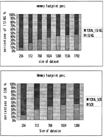
The reason why we pick why we pick the shape parameter k as 2 and the scale parameter

6 as 1, we concluded the two specific application and judged different situations while

the size changed from Figure 4.

o n o c Q '0 90% 80% 7(M 60% 50% 40% 30% 20% 10% JUS'

11

rarrory footprint perc.

IT0TALJSIN3 11 SINS

256 512 768 1024 1280 1536 1792 size of dataset

100%| o o CD a as c KJ a i

80%

70%

60%

50%

40%

30%

20%

10%

Itenwy footprint perc.

ITOWLJCR [SCR

512 768 1024 1280 Size of datasize

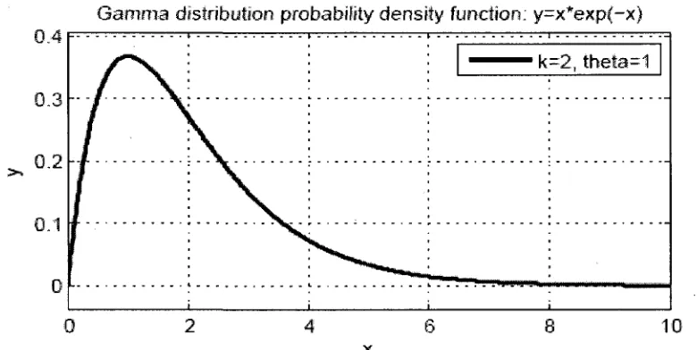
For calculating the low bound and high bound, we used the assistant tool MATLAB, to

draw the graph and get the figures at two extreme bounds. Like the Figure 6 below, we

settle the cursor on the cumulative distribution function chart and move it to get the right

figure at 0.2 and 0.95, then we map the x to the probability density function chart. Let

them cover the 20% and 95% of the total area.

Gamma distribution probability density function; y=x*exp(-x)

0.3-0.2

0.1

0

1 - - " - - - " - • • : • i • • _ • : • - . . . . . : . . . .

i i

i

--2, ihela=t

4 8 x

8 10

Gamma distribution Cumulative distribution function: y="l-exp(-x)-x*exp{-x)

Figure 5. The (PDF) probability density function and (CDF) cumulative distribution

4.2.2 Interval Setting

For deciding the interval of checkpointing, several papers [1][2][3] discussed optimal

intervals in the context of failure tolerance, the first was brought up in early 1974 given

an explicit formula Topt = V25M [ 1 ] where 8 is the time to write a checkpoint file, M is

the mean time between system failures (MTBF, it involves the whole aspects of system

such as CPU, memory, power cable etc.), and Topt is the optimum compute time between

writing checkpoint files. But its restriction is this model completely fails to predict

simulation results for small M. As for that reason, the second paper brought up in 2003,

by Young and claimed that Topt = •N/25(M + R) - 5 [3] to be an excellent estimator of

the optimum compute interval between restart dumps for values of (T +S)/M < — at the

end, where R be the restart time. In 2009, chen etal[\] pointed out the optimal

checkpoint intervals heavily depend on some system parameters, such as the time to place

a checkpoint, the time to recover from a fault, the fault arrival rate, and the user specified

parameters, like user defined timing constraints. Setting the intervals could influent the

system availability and task execution time.

We picked up the first formula to help us setting interval for our simulator. The reason is

we need to roughly predict the interval, although the model did not count the failure

probability. The MTBF as its definition is the mean time between failure for individual

components (e.g., processors, disks, memories, power supplies and networks). A large

leads to frequent individual failure. For components mentioned above, they all have an

operational lifetime measured in years. There are three different component reliability

levels: MTBFs of 104,105,106 hours. In particular, the IBM BlueGene/L system with

65536 nodes is expected to have an MTBF of less than 24 hours [4]. We followed the

graph and select the MTBF under the reliability level of 10s hours, with 128 nodes

involved in our simulation system around 200 hours. So in our case, the optimal

checkpoint interval would be set following the formula:

Topt= V25M = 20VS =20 J^-+ 0.5

V 70

S

:i to

140 120 I0O

-fe » h

60

\-40

20

V

10.000

joaooo

UJOO.OOO

*

\ ToraFLOPS

1 \

i \

-\

p i — i — I I I I

i»o

~r-t+»t-t-..iM>«

'\Pet-aFLOPS.

10000 IOWO0

System Size (number of nodes)

Figure 6. MTBF chart under different reliability level. [4]

every cases, thus we try to make our simulation more close to the real situation by adding

the normal distribution (Gaussian distribution) on the base interval setting and fix the

confidence limit o2 to let the probability density located between the confidence limits.

The normal distribution is Tmt~ldu,52) a n^ after expanded it is the formula with

variable x related with ju and a2, with ju be the median value of the bell curve and

o2 be the variance, here we define the a2 be around two to let the probability density

would reach 99.5% between the variances.

>(*)-1

542K exp

•(x-jif 2S2

M

{ M = 0,S2=1 )

CO

o

O

o o

/ • • •

\

,/ . / !

-n, v 2.1%Jk 2.1% _0.1%

- 3 a -2o - l a _{lcr 2a 3a}

Figure 7. Probability density function of normal distribution [12]

So far, we have done checkpoint overhead part and for migration and restart time we need

to clarify them. The migration time is not depending on the number of nodes, but linearly

storage to target nodes.

Migration cost = ^ - +7^ [21]

W

This formula was developed by Peiyu Cai [21]. (W is the write speed of stable storage

during the migration and for current technique we take 30MB/s, and Tmjn is the base time

which represents the basic overhead.) And for restart cost, that time on local node is

constant. Its cost relies on putting images to the node memory, once the migration done

transfer, the time to restart just short within one second.

4.3 Checkpointing Scheme by Migration with Checkpointing at Application

Level

As the original Scojo-PECT does not have checkpoint/migration support, the original

idea to introduce migration based on checkpointing is to fill fragmentations which were

created during the jobs being scheduled and find out the improvement of the scheduler

performance like average relative response time. The original scheduler handles the slice

by a series of operations such as release preempted jobs' memory, calculate free

resources, search preemption queue, waiting queue and apply backfill strategy if

possible.

As Peiyu Cai discovered mainly four cases on system level before [21], we did some

investigations on the application level on his basis. After investigating the scheduler, we

checkpointing. We reached a conclusion that to take better use of the free resources and

fill up the fragmentations, we could achieve it through backfilling (get jobs in the rear

position ahead) and migration (put jobs run on other free resource at the same time or at a

later time).

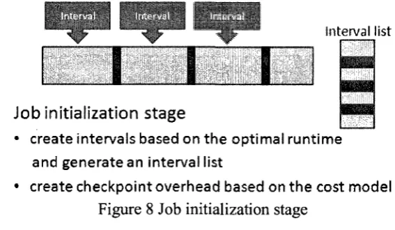
Generally, the application level checkpoint extension has three main stages:

1. Job initialization stage, see Figure 8. We figure out the places where we need to insert

our checkpoint intervals (create intervals based on the runtime) and generate an

interval list to hold them in time order and meanwhile calculate checkpoint overhead

based on the cost model.

In;= rt f J|

Interval list

I I I

Job initialization stage

• create intervals based on the optimal runtime

and generate an interval list

• create checkpoint overhead based on the cost model

Figure 8 Job initialization stage

2. Create next checkpoint event stage. As the scheduler processed jobs slice by slice and

generally jobs can be started either at the beginning or the middle of slice. So we

summarized two places we create the checkpoint event. 1) The beginning of slice, at

that time all the jobs we prepared to run in the particular slice, each has their own

jobs start from the beginning of slice.

3. Handle checkpoint event stage, see Figure 10. In this stage, we are going to discover

the chance to take advantage of migration based on checkpointing. We have two

kinds of queues here dealing with checkpointed jobs and selecting jobs for migration.

One is the reserve queue (It holds the checkpointed jobs) and the other is the

candidate queue (It holds the jobs which are able to run on the free resources at the

checkpoint time).

When reaching the checkpoint, a couple of things will be done. 1) Stop job and add

checkpoint overhead to simulate the checkpoint process. 2) Move the checkpointed

job into reserve queue. In reserve queue, a comparison function will pick out the

candidate jobs (could run on free resources) for migration and move them from

reserve queue into candidate queue. 3) The original scheduler do schedule first (try to

find out any non-type backfill), and right away migration operation will be done to let

jobs in candidate queue run on the free resources again.

The whole process of the simulation will contain such terms:

Reserve queue, it will hold the checkpointed jobs.

Candidate queue, it will hold the jobs which are able to run on the free resources at the

checkpoint time.

Application level interval list, it will hold the interval event based on jobs and sort it by

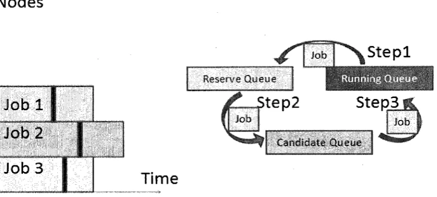
4.4 Extended Scheduling Algorithm

We only gain benefits based on the migration stage. In this chapter, we will focus on

talking about migration phase of handling the checkpoint event stage.

During us dealing with the checkpoint event, we can classify them into several steps, see

Figure 9:

The first step: get jobs from running queue and add them to the reserve queue, which is

used to hold the checkpointed jobs. And then let the original scheduler do schedule first

(The schedule function normally checks preemption queue, waiting queue of own job

type and other job types). We only extend the original scheduler and will not affect the

original decision.)

The second step: in the reserve queue, we compare the nodes of jobs with the total free

nodes in the cluster at the checkpoint time and pick out jobs which are able to run to the

candidate queue.

The third step: try to assign free nodes to candidate jobs of candidate queue. For each job,

if free resources are not the same as the original ones, do migration; if it is, run the

Nodes

Job 1

Job 2

Job 3

^ T job ^ * V Ste p 1

Reserve Queue

5tep2

Rjnnns?

StepH,

Job

Candidate Queue

Time

Figure 9 Migration stage

After we extended the original scheduler, we could have more flexibility on using free

resources, as we have more chance to backfill and migration. We deal with the situation

in Figure 10 like the following:

1) Job 2 will finish first, and the scheduler will search the preemption queue, waiting

queue of its own type and then waiting queue of other types to see if any jobs

could be backfilled. For this case, no other jobs can run.

2) Job 1 will have checkpoint, it will be moved from running queue and added to

reserve queue, and the original scheduler will do schedule (check preemption

queue, waiting queue of own job type and other job types). Later in this case, as

the free resource have been used by Job 3 (non-type backfilled), Job 1 will wait in

reserve queue.

3) Slice ends and change to another type of slice, Job 3 is preempted but can

4) Job 3 finishes and it will do the same operations as Job 2 did.

5) Job 4 will checkpoint, at this time it will also be added to reserve queue from

running queue, and the original scheduler will do schedule (check preemption

queue, waiting queue of own job type and other job types). Then job 1 and job 4

in the reserve queue will be moved to candidate queue because this time the free

resource are enough for them to run, and the last they are added to running queue

and start to run. Here Job 1 migrates to other resources as Job 4 prefers to run on

its original nodes.

N o d e s

J o b l

Job2

I

I

Jo-;-',

T i m e

slice e n d

N o d e s

m^m

backfilled

•H

•

s l i c e e n d

1

ReserveQ.

J o b l

Nodes ReserveQ C a n d i d a t e Q

W#M

w&n

t

I "

| j o b 4

J o b l

• »

11111

i t i migrated j o b

L... ! .Tiroe

slice e n d

Figure 10 Migration & Backfill

The main algorithm of doing migration is like the following:

case(APPCPevent){

job = getEventJob(APPCPevent); stop(job);

add To reservedQ(job); // reservedQ is a list that holds checkpointed jobs and let them hang on and wait.

Schedule(); // original Scojo-PECT scheduler function.

} // by here all possible jobs can be backfill'd or non-type backfilled will be backfilled.

for (all job in reservedQ) { // this is try to fill some of the jobs back migration supported, if (currentFreeNodes>=jobNodes) {

add to cahdidateQ(job) // jobs may back to run in own slice, if own position taken by backfilled jobs, perform "in slice" migration.

}

for (all job in candidateQ) {

restart (job);

}

else if(freeNodePosition = originalNodePosition) {

run(job) // no job takes its original position, back to run normally.

}

}

For this heuristic of selecting candidate jobs, in our extension, we always pick out the

jobs suit best in the candidate queue to fit the resource, and keep assigning resources to

jobs until the free resources have been taken used of (here may leave small number of

resource idle).

In our simulation, the heuristic for job selection does not affect the complexity of original

scheduler. Because the selection heuristic has already been merged into original one

which is using easy to fit or called first fit. The adoption of heuristic for job selection did

affect the execution time, its original runtime costs thirteen minutes for one run and the

5. Experiment and Result Analysis

In this chapter, we are going to introduce the experiments on our modified scheduler. The

experiment aims to test the fitting of the modified algorithm on handling jobs. We first

introduce the experiment environment in 5.1, and then propose the test cases in 5.2 and

deliver the testing results in 5.3 and final summarization on the observation from the

experiments.

5.1 Experiment Environment Setup

We used our own laptop for the testing environment. Its configurations are:

CPU: Intel Dothan 1.73GHz (One processor)

Memory: 2 Gigabytes DDR 533

Operation System: Microsoft XP SP2.

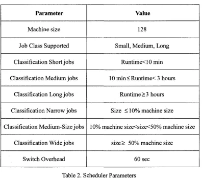
5.1.1 Workload Modeling

In our simulation, we only use the Lublin-Feitelson statistical workload model [19] which

is the best-available synthetic workload model (it includes sequential jobs, correlations

between runtimes and sizes, and varying inter-arrival times at different times of the

day/night). All workloads comprise of 10000 jobs. The other detailed parameters are listed

in table 2.

As in this event-based simulator, jobs are generated based on Lublin-Feitelson Model and

submitted. Therefore there would be different circumstances, like a job may end up

during the slice or exactly at the end of slice although these situations rarely happen.

While we still need to take this into consideration no matter whether it will give the

positive affection or the negative affection.

Parameter

Machine size

Job Class Supported

Classification Short jobs

Classification Medium jobs

Classification Long jobs

Classification Narrow jobs

Classification Medium-Size jobs

Classification Wide jobs

Switch Overhead

Value

128

Small, Medium, Long

Runtime<10min

10 min<Runtime< 3 hours

Runtime > 3 hours

Size < 10% machine size

10% machine size<size<50% machine size

size> 50% machine size

60 sec

Table 2. Scheduler Parameters

5.1.2 Evaluation Plan

The goals of these tests are trying to reveal the relation of relative average response time

Some terms we need to specify related to the results first:

Response time: it defines as the time span from the job was submitted to the job finished.

Runtime: it defines as the time period when the job starts to run and finishes running.

Relative response time: it represent as the ratio for the average response time and the

runtime.

In the test, we use different seed parameters. We are going to choose 7, 31, 13, 23 in

addition to original one 71. The reason why we are trying to use different seeds number

is the seed as a random parameter worked in Lublin-Feitelson model, it control the

function when generating jobs, filling them with different correlation of runtime and size.

It also changes the memory size of each job. So different seed may have different jobs

Work Load Seed 71 Seed 23 Seed 31 Seed 13 Seed 7 % ofJobs

Nshort

64

65

63

64

64

Nmed

19.5 19 20 19 20 Nbng 16.5 16 17 17 16

% of Work

Wshort

0.5

0.5

0.5

0.4

0.5

Wm ed

26 27 25 26.5 26 Wlong 73.5 72.5 74.5 73.1 73.5

Avg. Job Size

^short 9 9 9 9 8 ^med 17 17 16 17 17 ^long 19 20 20 20 21 Avg. Inter-Arrival Time (sec) 810 1038 860 798 840

Table 3 Characteristics of synthetic workloads

As we implemented checkpoint/migration, we will also make some combinations to test

the benefit purely from the migration stage rather than compare the checkpoint/migration

stage with the original simulation. Thus, there will be three cases: original, checkpoint

without migration, checkpoint with migration.

5.2 Experimental Results

The experimental results for the different cases with different seed numbers are showed

Relative Response Time(Long) Seed=71

16 -.

14

1 Q

-1 Z 1 ft

-o 6 4 2

-u

i .' '

— . ' • AVG U 14.56 14.53 ; "*r AVG LA 8.2 8.02 BNoCP_NoMG •CP_MG 20

-l b •

l u •

5

-u

HNoCP_NoMG

•CPJTC

R e l a t i v e Response Time(Medium)

— r » j

1

AVG MN

6.78

6.04

AVG

mm

1 1 . 6

1 1 . 5 7

•

AVG MW

16.81 16.78

Seed=71

h — | X: '

t< *

AVG HA

8.61 8.23

• N o C F _ M G

• C P mG

Figure 11 Relative Response Time for long and medium jobs at seed 71

In Figure 11, we can observe that the overall relative response time get improved 2.20%

for long jobs and 4.41 % for medium jobs, even with the wide jobs performed very badly

Relative Response Time(Long) Seed=31

Relative Response Time (Medium) S e e d ^ l

•NoCPJIdIG

aCP MG

Figure 12 Relative Response Time for long and medium jobs at seed 31

In Figure 12, we can observe that the overall relative response time get improved 1.21%

Relative Response Time(Long) Seed-7

20

1 cr

-I D

1 1 " )

1U

5

-0 •

BNoCP_NoMG

• C P J I G

rm

i ''' * pjp^if

AVG LN

7 . 2 8

6 . 9 9

-•'••• b j i j j

SH

rV;J;H

1 1 . 7 2

10.73 _ ^

m •••

I

.;\;;;HH

Relative Response Time(Medium) Seed-7

1 6 -I 1 A -1 4 1 0 -i n .

1U O 6 4 2 -U •NoCP_NoMG

@C P J I G

f • . . . - . . . -1

t ,

AVG MN

6.5

5.61

AVG MM

1 1 . 4 8

1 1 . 2 6

H

AVG MW

1 5 . 1 1

14.89 ' AVG HA 8.4 8.23 BNoCP_NoMG

BCP KG

Figure 13 Relative Response Time for long and medium jobs at seed 7

In Figure 13, we can observe that the overall relative response time get improved 1.06%

R e l a t i v e Response Time(Long) Seed=23

°NoCP_NoMG

•CP MG

R e l a t i v e Response Time(Medium) Seed=23 12 -.

1 n .

1U o c 0 4 • 2 -n . u HNoCP_NoMG mCP_IG I —

•

#i

1 \

AVG MM 8.19 7.64 - . AVG MW 11.33 11.32

*** 1

AVG MA

6.05

5.8

•HoCP_NoMG

BCP_MG

Figure 14 Relative Response Time for long and medium jobs at seed 23

In Figure 14, we can observe that the overall relative response time get improved 1.64%

Relative Response Time (Long) Seed=13 16

-1/1

-l^i

LC

10 -O " K 4 2 -o • BNoCP_NoMG MCP_MG

• * " " ' "

™ . , ™™ „ - , .

" " "

AVG LN

5.5

4 . 9 6

1=

Jt"

t . i i l l :: Mil

^B

..;..•

R e l a t i v e Response Time (Medium) Seed=13

30 -I

ZU

1 c; 1 3

1 r*i _

1U 5 u -BNoCP_NoMG aCP_MG .

t'*'wm

™^

'^';"BBI

?

- ' f c

'

!r

''-1

•;;'( l i l

.'

;

: jlj

V/fB

Figure 15 Relative Response Time for long and medium jobs at seed 13

In Figure 15, we can observe that the overall relative response time get improved 1.74%

Relative Response Time under seeds

Figure 16 Relative Response Time under different seeds

In Figure 16, we can observe that under different seeds the improvement of medium jobs

is around 4% at average and long jobs is around 1.5% at average, as the reason long jobs

are wider and medium jobs could take better use of checkpointed long jobs.

5.3 Result Analysis

Here we are going to discuss the efficiency of optimization. We will focus on the

improvement on the average relative response time under different situations.

The application level checkpoint approach in our simulation generally insert regular

checkpoint intervals in each job, which was calculated by program depend on their

going in slice after slice, in each slice jobs are taking up resource at certain time, and

some application level checkpoint intervals may happen at the same time but with very

mere chance. Most situations will be one job does the checkpoint operation while other

jobs are executing normally.

From the results, we could obtain that wide jobs are not easy to get checkpoint and

migrate, as they have to wait for enough resource to have itself to be executed. If we just

look at the narrow and medium jobs, the performance will be better. This also means that

long jobs will have less chance to take advantage of checkpointed medium jobs, as the

long jobs are wider. Also it means the medium jobs will have more chance to take better

6. Conclusion and Future Work

6.1 Conclusion

In this thesis, we have presented a job scheduling approach which employs application

level checkpoint and migration scheme on the original Scojo-PECT to tune up the

performance. As expected, this approach improves overall relative response time for both

medium and long type jobs, especially for the narrow and medium-size jobs. Specially,

the thesis has these contributions:

1) We implemented the application level checkpoint/migration as an extension to the

original scheduler;

2) We found out that application level checkpoint/migration improved the relative

response time a little;

3) We discovered that wide jobs usually are difficult to be migrated after being

checkpointed, as it will need to wait for enough free resource to resume its former

checkpointed work.

4) Narrow jobs are more suitable to use application level checkpoint as they require very

little resources, and thus get greater improvement. The reason is that, as the total

resources fixed, narrow jobs are more flexible to take use of free resources than other

size jobs. .

6.2 Future Work

selecting different algorithms to choose suitable jobs in candidate queue. Currently we

just tried the greedy algorithm and are not sure whether it produces the best combination

ofjobs.

Other works may be that we try some other impact factors, like we use real traces which

have different job type ratio and use different inter-arrival times. What is more, we could

also try with smaller job sizes because in the experiments we proved that the wide jobs

Reference

[1] Nianen Chen .Shangping Ren "Adaptive Optimal Checkpoint Interval and Its Impact

on System's Overall Quality in Soft Real-time applications" Symposium on Applied

Computing , Proceedings of the 2009 ACM symposium on Applied Computing,

2009.

[2] John W. Young "A First Order Approximation to the Optimum Checkpoint Interval"

Communications of the ACM, 1974

[3] John Daly "A Model for Predicting the Optimum Checkpoint Interval for Restart

Dumps", Springer Berlin / Heidelberg, 2003

[4] Petrini, F. Davis, K. Sancho, J.C'System-level fault-tolerance in large-scale

parallel machines with buffered coscheduling", Proceedings of 18th International

Parallel and Distributed Processing Symposium, 2004.

[5] Silva, L.M. Silva, J.G. "System-Level versus User-Defined checkpointing",

Proceedings on Seventeenth IEEE Symposium 1998.

[6] Schulz, M. Bronevetsky, G Fernandes, R. Marques, D. Pingali, K. Stodghill,

P. "Implementation and Evaluation of a Scalable Application-level

checkpoint-Recovery Scheme for MPI Programs", Proceedings of the ACM/IEEE

SC2004 Conference Supercomputing, 2004.

[7] Stellner, G "CoCheck: checkpointing and process migration for MPI" Proceedings of

IPPS '96, The 10th International Parallel Processing Symposium, 1996.

Parallel-Job Scheduling, High Performance Computing and Communication

(HPCC), Houston, LNCS 4782, Springer Verlag, Sept. 2007.

[9] A.C. Sodan, "Autonomic Share Allocation and Bounded Prediction of Response

Times in Parallel Job Scheduling", Seventh IEEE International Symposium on

Network Computing and Applications, July 2008.

[10] A.C. Sodan, Loosely Coordinated Coscheduling in the Context of Other Dynamic

Approaches for Job Scheduling—A Survey, Concurrency & Computation: Practice

& Experience, 17(15), Dec. 2005, pp. 1725-1781.

[11] Gamma Distribution. http://en.wikipedia.org/wiki/Gamma_distribution

[ 12]Normal Distribution. http://en.wikipedia.org/wiki/Normal_distribution

[13]A.C. Sodan, Adaptive Scheduling for QoS Virtual-Machines under Different

Resource Availability—First Experiences,_Job Scheduling Strategies for Parallel

Processing (JSSPP), 2009.

[14] Condor System, University of Wisconsin, http://www.cs.wisc.edu/condor/overview/

[15]C3 (Cornell Checkpoint (pre)Compiler) System, Department of Computer Science,

Cornell University, http://www.cs.cornell.edu/~stodghil/papers/ipdps05.pdf

[16] Paul H Hargrove, Jason C Duell, Berkley lab checkpoint/restart (BLCR) for Linux

clusters, Journal of Physics: Conference Series 46 (2006), pp. 494-499.

[17] John Paul Walters and Vipin Chaudhary, Application-Level Checkpointing

Techniques for Parallel Programs, Springer-Verlag Berlin Heidelberg, 2006

Practice and a Direction Forward in Checkpoint/Restart Implementations for Fault

Tolerance, 19th IEEE International Parallel and Distributed Processing Symposium

(IPDPS'05), 2005

[ 19] Feitelson Workload, http://www.cs.huji.ac.il/labs/parallel/workload/logs.html

[20] Colt, Open Source Libraries for High Performance Scientific and Technical

Computing in Java, http://acs.lbl.gov/~hoschek/colt/

[21]Peiyu Cai, Extending Scojo-PECT by migration based on system level

Appendix

In this appendix, we are going to test the proper migration and backfill functionalities of

the extended scheduler in the simulation.

Test Parameters

Description of testing parameters

Job type definition:

Small jobs < lOmin

1 Omin < < Medium jobs < 3 hours

Long jobs > 3 hours

Interval setting: 800 sec, the reason we choose 800s here is to make sure the small job

will be skipped as we do checkpoint and migration only on medium and long type jobs.

Checkpoint overhead: 3 sec. time costs doing the checkpoint

Average relative response time (ARRT), its definition is the ratio of the average response

time compared with its optimum runtime and the smaller number the better result.

Test Example

The job have several attributes, job submit time, job runtime, optimal node for job, job

memory size for application level checkpoint approach it also have the two other

SimpleJob(0, flex, new SimpleTime(O), Serialruntime, Nopt, Nmax, Nmin, Memory size,

config)

We manually created 6 jobs and arranged the submission time for each at different points

by setting up the parameters after calculation. After analysis the debugging process, we

could find the checkpoint/migration operation at the right decision points. This could

show that we have employed our implementation correctly according to the algorithm we

have proposed before. The detailed can be expressed like below:

Case Codes

if(i==0) //Serial run time/(nodes*0.65) = actual run time tmpJob =

new SimpleJob(0, flex, new SimpleTime (0), 24876, 128, 128, 128, 10, config);//299 else if(i==l)

tmpJob =

new SimpleJob(l, flex, new SimpleTime(80), 24876, 128, 128, 128, 10, config);//299 else if(i==2)

tmpJob = new SimpleJob(2, flex, new SimpleTime(lOO), 32045, 29, 29, 29, 240, config);//1700

else if(i=3)

tmpJob = new SimpleJob(3, flex, new SimpleTime(180), 84500, 99, 99, 99, 1024*3, config);//1300

else if(i==4)

config);//20000

else if(i==5)

tmpJob = new SimpleJob(5, flex, new SimpleTime(600), 1300000, 100, 100, 100, 1024*3, config);//20000

MATLAB Code for Calculation of Checkpoint File Size

Some codes in MATLAB using to draw the probability density function and cumulative

distribution function of gamma distribution are shown below:

syms x yl y2;

yl=x*exp(-x);

y2=l -exp(-x)-x*exp(-x);

subplot(2,l,l);

h=ezplot(yl,[0,10]);

title('Gamma distribution probability density function: y=x*exp(-x)');

legend('k=2,theta=l');

ylabel(y);

set( h, 'LineWidth' ,2 );

grid on;

subplot(2,l,2);

h=ezplot(y2,[0,10]);

title('Gamma distribution Cumulative distribution function: y=l-exp(-x)-x*exp(-x)');

legend('k=2, theta=l');

ylabel('y');

Vita Auctoris

NAME: Jiaying Shi

PLACE OF BIRTH: JiangSu, P.R. China

YEAR OF BIRTH: 1982

EDUCATION: Houcheng High School, Zhang Jiagang, JiangSu, China

1997-2000

Nanjing University of Technology, Nanjing, China

2000-2004

University of Windsor, Windsor, Ontario, Canada