Optimizing road test simulation using neural network modeling techniques

University of Windsor University of Windsor

Scholarship at UWindsor

Scholarship at UWindsor

Electronic Theses and Dissertations Theses, Dissertations, and Major Papers

2005

Optimizing road test simulation using neural network modeling

Optimizing road test simulation using neural network modeling

techniques

techniques

Jennifer Leslie Johrendt University of Windsor

Follow this and additional works at: https://scholar.uwindsor.ca/etd

Part of the Mechanical Engineering Commons

Recommended Citation Recommended Citation

Johrendt, Jennifer Leslie, "Optimizing road test simulation using neural network modeling techniques" (2005). Electronic Theses and Dissertations. 5248.

https://scholar.uwindsor.ca/etd/5248

O

R

T

S

U

N

N

M

T

By

Jennifer Leslie Johrendt

A Dissertation

Submitted to the Faculty o f Graduate Studies and Research through Mechanical Engineering

in Partial Fulfillment of the Requirements for the Degree of Doctor o f Philosophy at the

University o f Windsor

Windsor, Ontario, Canada

2005

Library and A rc h iv e s C a n a d a

B ib lio th eq u e e t A r c h iv e s C a n a d a P u b lish e d H eritage

Branch

395 W ellington Street Ottawa ON K1A 0N4 Canada

Your file Votre reference ISBN: 978-0-494-35074-4 Our file Notre reference ISBN: 978-0-494-35074-4

D irection du

P atrim oin e d e I'edition

395, rue W ellington Ottawa ON K1A 0N4 Canada

NOTICE:

The author has granted a non­ exclusive license allowing Library and Archives Canada to reproduce, publish, archive, preserve, conserve, communicate to the public by

telecommunication or on the Internet, loan, distribute and sell theses

worldwide, for commercial or non­ commercial purposes, in microform, paper, electronic and/or any other formats.

AVIS:

L'auteur a accorde une licence non exclusive permettant a la Bibliotheque et Archives Canada de reproduire, publier, archiver,

sauvegarder, conserver, transmettre au public par telecommunication ou par I'lnternet, preter, distribuer et vendre des theses partout dans le monde, a des fins commerciales ou autres, sur support microforme, papier, electronique et/ou autres formats.

The author retains copyright ownership and moral rights in this thesis. Neither the thesis nor substantial extracts from it may be printed or otherwise reproduced without the author's permission.

L'auteur conserve la propriete du droit d'auteur et des droits moraux qui protege cette these. Ni la these ni des extraits substantiels de celle-ci ne doivent etre imprimes ou autrement reproduits sans son autorisation.

In compliance with the Canadian Privacy Act some supporting forms may have been removed from this thesis.

While these forms may be included in the document page count,

their removal does not represent any loss of content from the thesis.

Conformement a la loi canadienne sur la protection de la vie privee, quelques formulaires secondaires ont ete enleves de cette these.

A

Growing interest in the use o f virtual simulation tools as part o f the automotive

product development process is driven by the need for automotive manufacturers and

parts suppliers to develop better quality products in shorter time at lower cost.

Component and full vehicle durability testing is one aspect o f product

development for which time savings can be realized. Traditionally, accelerated durability

simulations have been performed using full vehicles by driving physical prototypes on

specially designed road surfaces, simulating the vehicles’ service life. In the last thirty

years, durability testing has been accelerated in the laboratory environment where

measured vehicle excitation inputs have been edited to contain only the most damaging

portions. The goal of the current research is to advance the process further through the

use of high-fidelity virtual prototype durability simulations, which reveal the

consequences of design decisions made much earlier in the product development cycle

before the first physical prototypes are built.

Virtual durability full vehicle models are computationally complex. Linearizing

the individual models o f nonlinear components such as shock absorbers and elastomeric

bushings has been a typical method used to simplify the vehicle model. The focus of the

current research is to develop a methodology to increase the fidelity of these nonlinear

component models using computationally economical techniques, thus increasing the

precision of the results of the full vehicle model and the speed at which the results are

Neural networks are mathematical models that possess the flexibility and

computational efficiency desired for this application. These models are capable of

generalizing component behaviour using training data that represents the full range of

component behaviour that is to be modeled.

The current research describes the methodology required to develop and

implement neural network models o f nonlinear automotive components into simplified

and full-vehicle virtual durability models. The data used to train the neural networks

includes hysteresis effects that are not modeled with the methods currently available in

the multibody dynamics software package. Correlation of the results of the virtual

durability simulation with the laboratory test results is performed to show the validity of

A

The author gratefully acknowledges the support, inspiration, and dedication o f her

academic and industrial supervisors, Dr. Peter R. Frise and Mr. Mohammed A. Malik.

Together, they not only provided solid guidance during the course o f this research, but

also the trust and encouragement necessary to foster independent study. As people,

engineers, and educators, they are wonderful mentors, role models, and friends.

Thanks to DaimlerChrysler Canada Inc. for their generosity of time and resources

during this research project. Access to the equipment and personnel o f the University of

Windsor/DaimlerChrysler Canada Automotive Research and Development Centre made

this project possible.

The author expresses her deep appreciation for the generous funding of the

Natural Sciences and Engineering Research Council of Canada and DaimlerChrysler

Canada Inc. through the Industrial Post-Graduate Scholarship program.

I dedicate this work to my family and friends. George’s love and encouragement

has motivated me through the challenging moments and helped me celebrate each small

success along the way. I am grateful that Jennifer and Jonathan have always been my

biggest supporters. Throughout our years together, we have learnt that the potential of

our family unit is greater than the sum of its individual parts. We manage our triumphs

and tribulations better than any one of us could on their own. I can’t neglect to mention

our four-legged family members, Jake, Heidi, and Bentley. I was always grateful for

their loyal companionship and laughable antics. Finally, thanks to my parents for their

T

C

A bstract... iii

Acknowledgements... v

List of Figures...x

List of T a b le s... xxxi

List of A bbreviations... xxxiv

List of Sym bols... xxxv

1 Introduction...1

1.1 Product D evelopm ent...1

1.2 Vehicle Durability: Field and Laboratory Testing... 3

1.2.1 Fatigue and Durability T estin g ...3

1.2.2 Accelerated Durability Tests... 4

1.2.3 Road Test Simulation... 5

1.3 Virtual Durability Sim ulation... 6

1.4 Neural N etw orks...7

1.5 Research Objectives of the Present S tu d y ... 9

2 Literature Review... 11

2.1 Product D evelopm ent... 11

2.2 Durability and Road Test Sim ulation... 12

2.3 Modeling Nonlinear Components... 13

2.4 Using Neural Networks to Model Automotive Components... 15

3 T heory... 17

3.1 Vehicle Dynam ics... 17

3.1.1 Ride and Handling vs. D urability...17

3.1.2 The Role of Suspension Com ponents... 18

3.2 Elastomers... 18

3.2.1 Polymer Structure of Elastom ers... 18

3.2.2 Mechanics of Viscoelastic Behaviour...21

3.3 Introduction to Neural N etw orks...28

3.4 Designing Neural Networks...31

3.4.1 Methods of Construction...33

3.4.2 Activation Functions... 34

3.4.3 Scaling the Input and Output D ata...35

3.4.4 Number of Hidden Layer Perceptrons...36

3.4.5 Training and Validation Data S ets...37

3.4.6 Measuring the Performance of the N etw ork... 37

3.4.7 Determining Appropriate Weights and Bias Values...42

3.5 Using Neural Networks to Characterize Material Behaviour... 49

4 Applying Neural Network Modeling Techniques... 51

4.1 ADAMS Model Preparation... 52

4.2 ADAMS Model C om ponents... 53

4.2.1 Location and Orientation o f M arkers... 53

4.2.2 State V ariables... 54

4.2.3 ADAMS/View Function B uilder...55

4.2.4 ADAM S/Controls...57

4.2.5 Arrays and Filters...58

4.2.6 ADAMS Dampers...59

4.2.7 ADAMS B ushings...63

4.3 Modified ADAMS Com ponents... 67

4.3.1 Modified D am pers...67

4.3.2 Modified Bushings...71

4.4 ADAMS/Controls Plug-in M odule...76

4.5 Neural Network Construction... 78

4.5.1 Spline D ata...79

4.5.2 Hysteresis D a ta ... 86

4.5.3 Time History D ata...91

4.6 Co-simulation... 95

4.6.1 Sim ulink... 96

5.1 Neural Network Model o f a Shock Absorber Force-Deflection Spline...103

5.2 Neural Network Model o f a Shock Absorber Force-Deflection Hysteresis Curve ...109

5.3 Neural Network Results: Bushing Time Series Data... 116

5.3.1 Axial Force M o d el...120

5.3.2 Radial Force M odel...123

5.3.3 Axial Torque M odel...126

5.3.4 Conical Torque M o d el... 129

5.4 Implementation and Validation of Vehicle M o d el...132

5.4.1 Co-simulation Using a Neural Network Model o f a Shock Absorber Force versus Deflection Velocity Spline Curve... 133

5.4.2 Co-simulation Using a Neural Network Model of a Shock Absorber Force versus Deflection Velocity Hysteresis C u rv e...134

5.4.3 Co-simulation Using a Neural Network Model of Bushing Forces and T o rq u es... 140

5.5 Correlation: Laboratory and Simulation R esults... 174

6 Conclusions and Recom mendations...180

6.1 Conclusions... 180

6.2 Recommendations... 181

6.2.1 Neural Network D evelopm ent... 181

6.2.2 Neural Network Im plem entation... 182

Appendix A: Bushing Data A cquisition... 184

A .l Data Acquisition Overview... 184

A.2 Desired Data Preparation... 185

A. 3 Test S et-up ... 194

A.3.1 Fx, Axial Force Measurement Set-up...195

A.3.2 Fz, Radial Force Measurement S et-u p ...195

A.3.3 Tx, Axial Torque Measurement Set-up... 197

A.3.4 Tz, Conical Torque Measurement Set-up... 198

A.4 Data A cquisition... 199

A.4.2 Measurement o f Tx and Tz ...200

A.4.3 Iterations Results... 200

A. 5 Dataset selection... 213

A.6 Data S um m ary... 217

Appendix B: Neural Network Construction E xam ple... 227

B. 1 Nonlinear Function Approximation... 227

B . 1.1 Training and Test D a ta ... 227

B.1.2 Network Structure...228

B. 1.3 Neural Network D evelopm ent... 230

B.1.4 Results...233

B.2 Approximating A Nonlinear Function with Noise... 236

B.2.1 Training, Validation, and Test Data... 236

B.2.2 Network Structure...237

B.2.3 Neural Network D evelopm ent... 238

B.2.4 Results... 238

References... 241

L

F

Figure 1.1:

Figure 1.2:

Figure 1.3:

Figure 1.4:

Figure 1.5:

Figure 1.6:

Figure 1.7: Figure 1.8: Figure 1.9:

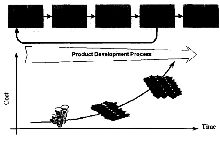
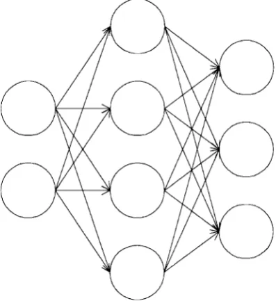
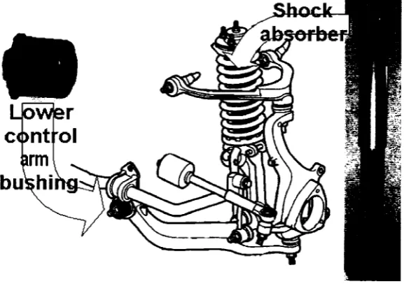
The traditional product development cycle can be an iterative process, with revisions occurring late in the cycle... 1 The cost of making changes during product development cycle grows dramatically with tim e... 2 The revised product development cycle allows for design iterations earlier in the process... 2 Vehicle on test at a corporate proving grounds. (Photograph courtesy of DaimlerChrysler Corporation.)... 4 Test vehicle on a road test simulator during the drive file development process. (Photograph courtesy o f DaimlerChrysler Canada Inc.)...5 Virtual durability simulation model of a road test simulator and a vehicle in ADAMS...6 Neurons receive and transmit signals in the brain...7 Signals flow through the neural network along the weighted paths 8 Front suspension components that will be modelled with neural networks are coloured red (front lower control arm front bushing, front shock absorber). [5]...9 Figure 2.1: Roles of participants in traditional product development [13]... 11 Figure 2.2: The front lower control arm bushing is oriented as shown with the X-axis

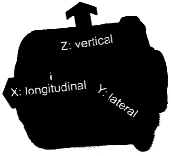
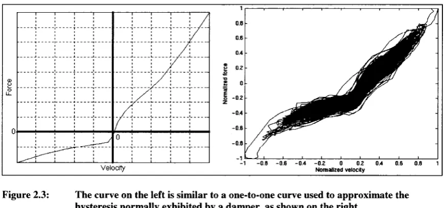
pointing towards the front o f the vehicle... 13 Figure 2.3: The curve on the left is similar to a one-to-one curve used to approximate

the hysteresis normally exhibited by a damper, as shown on the right 16 Figure 3.1: Polyisoprene is a polymer o f carbon (C) and hydrogen (H) atoms formed

into long chains of repeating units or “mers”. The polyisoprene “mer” is shown here repeating 'n' times. Polyisoprene is commonly called natural rubber... 19 Figure 3.2: The addition of sulfur to polyisoprene forms vulcanized rubber, an

elastomeric material commonly used in the manufacture o f automotive bushings...19 Figure 3.3: The glass transition temperature is the temperature at which the vulcanized

Figure 3.5: During viscoelastic relaxation, stress decreases as the strain is held

constant... 23 Figure 3.6:

Figure 3.7:

Figure 3.8:

Figure 3.9:

Figure 3.10:

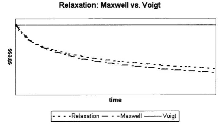
Figure 3.11:

Figure 3.12:

Figure 3.13:

Figure 3.14:

Figure 3.15:

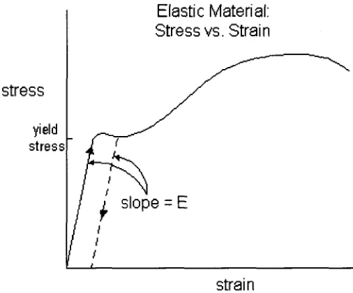
This is a typical stress versus strain curve for an elastic material that exhibits yielding. Note that when the material is loaded past the yield stress, unloading occurs along a parallel path (i.e. with the same slope and thus the same elastic modulus) to a state of permanent (plastic)

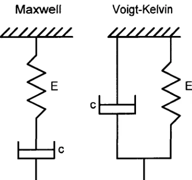
deformation... 24 The strain response lags the applied dynamic stress to a viscoelastic material as illustrated by the phase lag between the two signals... 24 Viscoelastic stresses exhibit a lagged strain response that develops into a hysteresis curve in a stress versus strain plot. The arrows indicate the progression o f time, such that loading and unloading of the specimen are shown... 25 The Maxwell and Voigt-Kelvin viscoelastic models use springs to model the elastic component of the behaviour (stiffness, E) and viscous dashpots to model the viscous behaviour of the material (damping, c)...26 The Voigt element better predicts strain during creep than the Maxwell element for which strain varies linearly during constant applied stress... 27 The Maxwell element better predicts stress during relaxation than the Voigt element for which stress is constant during constant applied strain. ...27 The biological neuron accepts signals from other neurons, processes the combined signal at the nucleus, and sends the resulting signal along axons downstream to other neurons [20]... 28 For negative values of the input variable, net, the output of the function

f(net) is either -1 . For positive or zero values of the input variable, net,

the output of the function f(net) is +1. The threshold nonlinearity function

[\,net > 0

is described mathematically by f , hreshold (net) = \ 29

[ - l ,n e t < 0

Figure 3.16: The threshold, hyperbolic tangent (tanh), and logistic functions are nonlinear activation functions commonly used in neural network design. The variable net is input to the activation function that acts as a trigger or firing threshold to produce an output. The continuous differentiability of the hyperbolic tangent, and logistic functions make them more desirable for neural network structures because this property will allow calculation of the back propagation o f the error during the training phase of network construction... 34 Figure 3.17: The network input data used in the simulation is scaled using the

maximum and minimum values of the training input data. The scale of the simulation outputs of the neural network is recovered using the maximum and minimum values o f the training data outputs... 36 Figure 3.18: The single perceptron employs a linear activation function to estimate a

single output value from n inputs. It will be used to illustrate the concept o f optimizing the performance of the network during training... 39 Figure 3.19: In this example of the performance of a single layer network using a linear

activation function, the value o f the M SE is minimized for w*=0.75...40 Figure 3.20: The use of hyperbolic activation functions causes local minima to arise in

the performance minimization. The learning algorithm should be modified to ensure that the true optimal weight is found at the global minimum of the performance function...41 Figure 3.21: The Ith perceptron accepts n inputs and produces one output. Note that the

weights, w,j, and bias, £>„ are the variable parameters that are adjusted during training of the neural network... 43 Figure 3.22: The bias of the ith perceptron in Figure 3.21 can be replaced by an

additional input element, +1, and a corresponding weight, ...43 Figure 3.23: The output of t h e / h perceptron is weighted with Wy and passed to the /th

perceptron in the hidden layer, weighted with wid and passed to the kth

perceptron that resides in the output layer... 45 Figure 3.24: The value o f the weight, w, is adjusted by a rate proportional to the

gradient of the M SE curve. In this fashion, the optimal value, w*, is eventually reached after a sufficient number o f iterations...48 Figure 3.25: The network weights displayed in the histogram show the highest

concentration o f weights with small magnitude and form a bell-shape about the midpoint. Weights larger than about ten are undesirable due to the amplification effect on errors passing through that weighted path o f the network [37]...49 Figure 3.26: This normalized damping force versus normalized shock deflection

Figure 4.1: Data is passed to and from the ADAMS model from the Simulink

environment where the neural networks reside... 51 Figure 4.2: This example of a 90-90-90 Euler transformation illustrates three 90°

rotations about the z-, x ’-, and z”-axes, respectively, to transform the x - y

A A A

- z coordinate system into x - y - z coordinate system. In the ADAMS software, x - y - z represents the global coordinate system, and the marker

A A A

coordinate system, x - y - z , is said to have the orientation (90, 90, 90)

relative to the global coordinate system... 54 Figure 4.3: A control system monitors the output variables of a plant process.

Adjustments to the plant input variables are made by a controller to achieve output variables that are closer to desired values [8]...55 Figure 4.4: The transfer function, TFSISO_lp_filter, represents the low pass filter

used to filter the incoming damping force data has a cutoff frequency of 100Hz... 59 Figure 4.5: The damper exerts equal and opposite forces that act along the

line-of-sight between Sprung_mass.MARKER_3 and

Unsprung_mass.MARKER_4. The dialog box is used to define the bodies and the damping coefficient constant expressed in units of N-s/mm or a spline curve that defines the damping force with respect to the velocity of the shock absorber deflection... 61 Figure 4.6: The spline curve represents a nonlinear approximation of the damping

force with respect to the rate of deflection of the damper. Both force and velocity data have been normalized with respect to their maximum

respective values to protect proprietary data. Rebound or extension of the damper is produces a positive deflection velocity and damping force, while the jounce condition or compression of the damper produces

negative deflection rate and damping force... 63 Figure 4.7: The bushing exerts three translational and three rotational forces between

shaft.MARKER_4 and sleeve.MARKER_3. Note that the ADAMS bushing definition aligns the z-axis along the bushing’s axial direction. If the bushing is symmetrical, the x-axis and y-axis coefficients are identical. The dialog box is used to define the bodies and the constant stiffness and damping coefficients... 65 Figure 4.8: The dialog boxes for creation of state variables are shown. The damping

Figure 4.9:

Figure 4.10:

Figure 4.11:

Figure 4.12:

Figure 4.13:

Figure 4.14:

Figure 4.15:

Figure 4.16:

Figure 4.17:

Figure 4.18:

Figure 4.19:

ARRAY_dam pingj.nput (left) is an input array (U) that used to filter

damping_force_variable (input to ADAMS from MATLAB) using the

transfer function, TFSISO _lpJilter. ARRAY_filtered_damping is the output array (Y) from T F S IS O J p Jilter, the value of which is then used as the damping force... 68 The modified damping force definition calls upon the filtered value of the damping force that was input from MATLAB...69 The modified damping force acts along the line o f sight between the unsprung and sprung masses. It is defined to accept data from MATLAB input through the Controls Plug-in module...70 This figure shows the orientation of a bushing that is defined to produce three forces and three torques that act between an action and a reaction body (this example shows a shaft acting as the action body and a sleeve acting as the reaction body). Note the distinction between the axial direction (z-axis) and the two radial directions (x-axis and y-axis), indicating that the largest rotation occurs about the z-axis. Asymmetric bushings possess different bushing stiffness and damping properties in each of the two radial directions...72 The dialog boxes for creation of state variables are shown. The bushing axial force variable (left) acts as a placeholder for incoming data and must show a value o f zero (0). The x-axis deflection (right) is an example o f a variable that whose value will be calculated and output to MATLAB for processing. Note that it is a measurement of the x-component o f the relative translation vector between the markers... 73

ARRAY_axialJorce_input (left) is used to pass Axial_force_variable

(input to ADAMS from MATLAB) as input to the low pass filter (e.g.

TFSlSO _lpJilter). A R R A YJiltered_axialJorce contains the output of the filter, which is then passed onto the bushing force element... 74 The modified bushing force definition is defined by the filtered values of the forces and torques that were input from MATLAB... 74 The modified bushing force acting between MARKER_5 and

Figure 4.20: Figure 4.21: Figure 4.22: Figure 4.23: Figure 4.24: Figure 4.25: Figure 4.26: Figure 4.27: Figure 4.28: Figure 4.29:

The Network/Data Manager is the first graphic user interface that opens when using the Neural Network Toolbox. The user can create or import data and neural networks... 80 The 1-1-1 feed forward network defined in the graphic user interface accepts input data ranging from -1 to 1, trains using the gradient descent with momentum method (traingdm), and monitors performance using the

MSE. The activation function chosen for use in the hidden layer is the hyperbolic tangent while the output layer employs a linear function 81 The Network graphic user interface allows processing of the network, including viewing (shown), training (shown), simulating, and display of the weights and bias values... 82 The spline data points were separated into training and validation data sets as shown in the plot...84 The hysteresis curve that is based upon the ADAMS spline curve will be modeled using a time delay neural network structure... 87 The damping hysteresis data points were separated into training and validation data sets as shown in the plot. The validation points were randomly selected from the complete set o f thirty points on the hysteresis curve. Their locations on the hysteresis curve are shown here... 90 The Simulink model shows the flow of data during the co-simulation. The adams_sub block represents the ADAMS component of the model. In the example shown, the neural network estimated damping force is passed to the adams_sub block where the ADAMS solvers are employed to calculate the state of the system for the current time step. The input or excitation force, damper deflection, and damper deflection velocity are output and plotted together with the damping force. The damper deflection velocity is fed back and input to the neural network for

Figure 4.30:

Figure 5.1:

Figure 5.2:

Figure 5.3:

Figure 5.4:

Figure 5.5:

Figure 5.6:

Figure 5.7:

The Simulink library contains many sets of predefined blocks including function generators, plotters, transport delay, gains, summing, and signal multiplexers... 102 The spline curve is fitted to the measured shock absorber force versus deflection velocity data points. Note the differences in slope of the curve between jounce and rebound conditions. This curve will be modeled by a neural network...104 The 1-3-1 neural network was developed using all fifteen spline points for training and did not use early stopping. The training yielded an M SE of 0.0010... 105 The 1-5-1 neural network was also developed using all fifteen spline points and did not use early stopping. In this case, the training also yielded an M SE of 0.0010. Since the slightly more complicated network structure yielded the same performance as the simpler network, the simpler network structure of the 1-3-1 neural network is preferable to the

1-5-1 network without early stopping...106 The 1-5-1 neural network that was developed with early stopping could only utilize thirteen spline points for training and two data points for validation. The network performance during training was better than that of the networks developed without early stopping {MSE = 0.0006).

Further examination o f this network’s accuracy compared to the 1-3-1 network of Figure 5.2 is required before a model can be selected 106 The results of the 1-3-1 and 1-5-1 neural networks are shown with the ADAMS spline data. In general, the 1-3-1 network that was trained without early stopping models the ADAMS spline curve better, especially in the region of higher rebound velocity, where there are fewer training points available during training... 107 The weights of the 1-3-1 neural network that was trained without

validation data, shows that the weights range from about - 4 to 4. The compact range of the weights is desirable, but the low quantity of weights in the network prevents the ability of the histogram to take on a more distinctive bell-shape that is desirable of such a distribution... 108 The weights of the 1-5-1 neural network that was trained with validation data, shows the weights range from about -7 to 7. The increased range of the values of the weights makes it less desirable than the histogram of the

Figure 5.8:

Figure 5.9:

Figure 5.10:

Figure 5.11:

Figure 5.12:

Figure 5.13:

Figure 5.14:

The hysteresis curve differs from the spline curve in that the upper and lower branches correspond to different loading o f the shock absorber. The upper branch shows that a larger force is produced in the damper than the lower branch. The branches correspond to shock absorber motion

between maximum jounce velocity to maximum rebound velocity. A spline curve of shock absorber damping approximates the force produced regardless o f the direction o f loading. The hysteresis curve shown here was generated using the spline curve data used to model the shock

absorber in ADAM S...109 The 1-3-1 neural network was developed without early stopping using all thirty data points for training. The M SE achieved during training was 0.0010. Note that the hysteresis was not modeled by this network

structure. Instead, the model produces shock absorber forces between the upper and lower branches o f the hysteresis curve... I l l The 2-7-1 neural network was trained with all thirty data point and did not use early stopping. The M SE for the training data was 0.0010. The hysteresis is evident in the model, but does not follow the curve very well for jounce conditions (negative velo city)... 111 The 3-7-1 neural network also used all thirty data points for training and no early stopping. Again, the training yielded an M SE of 0.0010. The network shows better estimation of the hysteresis curve than the 2-7-1 model shown in Figure 5.10... 112 The 2-5-1 neural network was developed with early stopping, using twenty-seven points for training and three data points for validation. An

Figure 5.15:

Figure 5.16:

Figure 5.17:

Figure 5.18:

Figure 5.19:

Figure 5.20:

Figure 5.21:

The weights of the 2-5-1 neural network that was trained with early stopping range from about - 3 to 3. The distribution more closely resembles a bell-shaped curve compared to the 2-7-1 network shown in Figure 5.14... 114 The results of the 2-7-1 and 2-5-1 neural networks are shown with the original hysteresis data as the velocity is swept through from maximum jounce to maximum rebound. Both networks model the hysteresis curve

well, but the 2-5-1 model was selected due to its better distribution of weights per the histogram shown in Figure 5.15. The discrepancy of both curves to model the hysteresis data at the far left of the plot is due to the use o f zero initial time delay values for the networks’ input...115 Bushing force and translational deflection data was measured in the axial and radial directions. Bushing torque and rotation deflection data was measured in the axial and radial directions. Radial torque is also referred to as conical torque. Since the bushing was symmetric, the models o f the radial force and torque can be applied in two perpendicular radial

directions during co-simulation... 116 This plot illustrates typical results of the calculation of the sensitivity of the axial force with respect to the ten inputs. In general, it was determined that both the axial and radial bushing forces showed higher sensitivity to zero time-step delay displacement and velocity inputs compared to the acceleration and the one- and two-time delay inputs of the displacement, velocity, and acceleration... 118 This plot illustrates typical results of the calculation o f the sensitivity of the conical torque with respect to the ten inputs. In general, it was

Figure 5.22: The ability of the 2-3-1 neural network to estimate training, validation, and test data of the axial bushing force is shown here. Note the concentration o f the cluster of test data points within the training and validation data point clusters. This illustrates the network’s ability to model data to which it was not exposed during the training phase and thus shows the efficacy of the neural network approach...123 Figure 5.23: The weights o f the 2-3-1 radial force neural network model exhibit a

bell-shape concentrated about zero ranging from -5 to 4 ... 124 Figure 5.24: The ability o f the 2-3-1 neural network to model the bushing radial force

is shown here in the time domain. The good correlation for the training (top) and validation data (middle) illustrates the success o f the network to generalize the training and validation data sets during the training process. The success of the network to estimate the test data (bottom) shows the network’s ability to model the radial force produced during radial

translational bushing deflection that was not used during the training phase of network development... 125 Figure 5.25: The ability of the 2-3-1 neural network to estimate training, validation,

and test data of the radial bushing force is shown here. Note the concentration o f the cluster of test data points within the training and validation data point clusters. This illustrates the network’s ability to model data to which it was not exposed during the training phase 126 Figure 5.26: The weights of the 4-7-1 axial torque neural network model exhibit a

bell-shape concentrated about zero ranging from - 4 to 4 ... 127 Figure 5.27: The time histories o f the normalized axial torque from the training (top),

validation (middle), and test data sets (bottom) are shown for the 4-7-1 neural network model. The time delay network structure successfully generalized the axial torque response to bushing axial rotation during training. Once the network was successfully trained, it was then able to correctly estimate the axial torque from previously unseen input d a ta .. 128 Figure 5.28: The ability of the 4-7-1 neural network to estimate training, validation,

and test data of the axial bushing torque is shown here. Note the concentration of the cluster o f test data points within the training and validation data point clusters. This illustrates the network’s ability to model data to which it was not exposed during the training phase 129 Figure 5.29: The weights of the 4-7-1 conical torque neural network model exhibit a

bell-shape concentrated about zero ranging from - 4 to 7 ... 130 Figure 5.30: The time histories of the normalized conical torque from the training (top),

Figure 5.31:

Figure 5.32:

Figure 5.33:

Figure 5.34:

Figure 5.35:

Figure 5.36:

The ability of the 4-7-1 neural network to estimate training, validation, and test data of the conical bushing torque is shown here. Note the concentration o f the cluster of test data points within the training and validation data point clusters. This illustrates the network’s ability to model data to which it was not exposed during the training phase. The width o f the clusters is a result o f the small signal range relative to the axial force, axial torque, and radial force data...132 The Simulink model shows the method used to run the co-simulation using the spline look-up table and the neural network model o f the damping force. For the Simulink model shown, the neural network- estimated damping force is input to the “adams_sub” block...134 The random input shown was one of the signals used to excite the single degree o f freedom model during the co-simulation. A baseline response to the excitation was measured in ADAMS and then co-simulations using the spline and hysteresis neural network models were performed. The results are shown in Figure 5.34 to Figure 5.37...135 This portion of the time history plot of the shock absorber force generated in the co-simulation of the single degree of freedom model for both the spline (blue) and hysteresis (green) neural network models are shown in comparison with ADAMS model baseline (black). The neural network model estimates higher positive and negative peaks in the time history. This corresponds to the position of the hysteresis forces relative to the spline curve shown in Figure 5.8...136 The frequency plots of the shock absorber force generated in the co­

simulation of the single degree of freedom model for both the spline (blue) and hysteresis (green) neural network models are shown in comparison with ADAMS model baseline (black) from 0 - 4 5 Hz. The full time history of the response to the random input signal is used to calculate this plot. In general, the hysteresis model estimates higher amplitude signals

for most frequenciesfe .g .J '0.175 = 1.29 at 1 Hz 0.105

This agrees with the

Figure 5.37:

Figure 5.38:

Figure 5.39:

Figure 5.40:

Figure 5.41:

Figure 5.42:

This frequency plot of the shock absorber deflection generated in the co­ simulation of the single degree o f freedom model for both the spline (blue) and hysteresis (green) neural network models are shown in comparison with ADAMS model baseline (black) from 0 - 3 0 Hz. The full time history for the response to the random input signal is used to calculate this plot. The amplitudes of the spline and hysteresis models correlate well with the ADAMS model. At about 1 Hz, the amplitude o f the hysteresis

model is r ' 107 = 0.95 of the amplitude of the ADAMS baseline 139 V 0.118

The Simulink model shows that the axial displacement and velocity output from the ADAMS subsystem were used to calculate the axial bushing force and the axial rotation and angular velocity were used to calculate the bushing axial torque using the neural network models developed in

Figure 5.43:

Figure 5.44:

Figure 5.45:

Figure 5.46:

Figure 5.47:

The results of the co-simulation using neural network models o f both the front and rear axial bushing forces show that the neural network model correlates extremely well with the ADAMS simulation with regard to the normalized rear normalized bushing axial displacements. This portion of the results from 30 to 35 seconds contains the global peaks for the full 50 second simulation showing that the method developed in the present research provides a valid simulation over the entire range o f the physical phenomenon... 147 The frequency plots for the front normalized axial displacements were calculated using the full 50 seconds of road simulation data. The plots show good correlation between the ADAMS simulation and the co­ simulation using the axial force neural network model. The peak located at 0 Hz shows the results from the co-simulation results are about

= i .i 5 times (about 15% larger than) the ADAMS simulation

V 0.03

results, which corresponds to a small difference in the mean value o f the signal through the full simulation...148 The frequency plots for the rear normalized axial displacements were calculated using the full 50 seconds of road simulation data. The plots show good correlation between the ADAMS simulation and the co­ simulation using the axial force neural network model. The peak located at 0 Hz shows the results from the co-simulation results are about

= U 5 times (about 15% larger than) the ADAMS simulation V 0.03

Figure 5.48:

Figure 5.49:

Figure 5.50:

Figure 5.51:

Figure 5.52:

Figure 5.53:

Figure 5.54:

The frequency plot for the front normalized axial bushing force was calculated using the full 50 seconds of road simulation data. The plot shows good correlation for all frequencies between the ADAMS

simulation and the co-simulation using the neural network models o f both front and rear axial forces...152 The frequency plot for the rear normalized axial bushing force was

calculated using the full 50 seconds of road simulation data. The plot shows good correlation for all frequencies between the ADAMS

simulation and the co-simulation using the neural network models o f both front and rear axial forces...153 The results of the co-simulation using neural network models of both the front and rear axial bushing torques show that the neural network model correlates well with the ADAMS simulation with regard to the front bushing normalized axial rotation. This portion o f the results from 30 to 35 seconds contains the global peaks for the 50 second simulation showing that the method developed in the present research provides a valid simulation over the entire range of the physical phenomenon 154 The results o f the co-simulation using neural network models of both the front and rear axial bushing torques show that the neural network model correlates well with the ADAMS simulation with regard to the rear bushing normalized axial rotation. This portion of the results from 30 to 35 seconds contains the global peaks for the 50 second simulation showing that the method developed in the present research provides a valid simulation over the entire range o f the physical phenomenon 155 The frequency plot for the front bushing normalized axial rotation was calculated using the full 50 seconds of road simulation data. The plot shows good correlation between the ADAMS simulation and the co­ simulation using the axial force neural network model for all frequencies. ...156 The frequency plot for the rear bushing normalized axial rotation was calculated using the full 50 seconds of road simulation data. The plot shows good correlation between the ADAMS simulation and the co­ simulation using the axial force neural network model for all frequencies. ...157 The results of the co-simulation using neural network models of both front and rear axial bushing torques show that the neural network model

Figure 5.55:

Figure 5.56:

Figure 5.57:

Figure 5.58:

Figure 5.59:

Figure 5.60:

The results of the co-simulation using neural network models of both front and rear axial bushing torques show that the neural network model

predicts that the rear bushing reacts with a smaller negative torque than the constant coefficient stiffness and damping of the ADAMS bushing model. Despite this difference between the models, the rotation o f the rear

bushing correlates well (see Figure 5.51). This portion o f the results from 30 to 35 seconds contains the global peaks for the simulation...159 The frequency plot for the front normalized bushing axial torque was calculated using the full 50 seconds o f road simulation data. The plot shows that at 0 Hz the results from the co-simulation are approximately

13,2

J — = 0.82 times the ADAMS simulation results. This result corresponds

to the shift in mean value of the full 50 second signal compared to the ADAMS simulation...160 The frequency plot for the rear normalized bushing axial torque was calculated using the full 50 seconds of road simulation data. The plot shows that at 0 Hz the results from the co-simulation are approximately

/

J — = 0.82 times the ADAMS simulation results. This result corresponds

Figure 5.61:

Figure 5.62:

Figure 5.63:

Figure 5.64:

Figure 5.65:

Figure 5.66:

Figure 5.67:

Figure 5.68:

Figure 5.69:

Figure 5.70:

Figure 5.71:

Figure 5.72:

Figure 5.73:

The results of the co-simulation using neural network models of the conical bushing torques in both the X- and Y-directions show that the neural network model correlates well with the ADAMS simulation with regard to the normalized conical torque produced in the Y-direction. This portion o f the results from 30 to 35 seconds contains the global peaks for the 50 second simulation showing that the method developed in the present research provides a valid simulation over the entire range o f the physical phenomenon... 171 The frequency plot for the front bushing normalized conical torque in the X-direction was calculated using the full 50 seconds o f road simulation data. The plot shows excellent correlation between the ADAMS

simulation and the co-simulation using the conical torque neural network model for all frequencies... 172 The frequency plot for the front bushing normalized conical torque in the Y-direction was calculated using the full 50 seconds of road simulation data. The plot shows excellent correlation between the ADAMS

simulation and the co-simulation using the conical torque neural network model for all frequencies... 173 The ADAMS simulation and neural network co-simulation results

correlate well with the RTS laboratory data with regard to the normalized lower control arm angle. This portion of the results from 30 to 35 seconds contains the global peaks for the 50 second simulation...175 The frequency plot for the normalized lower control arm angle were calculated using 50 seconds o f road simulation data. The plots show that the ADAMS simulation and all neural network co-simulations correlate well with the RTS laboratory results for all frequencies...176 The ADAMS simulation and neural network co-simulation results for the damping force show higher positive peak forces and a slight upward shift in the average load towards zero compared to the RTS laboratory data. This portion of the results from 30 to 35 seconds contains the global peaks for the 50 second simulation... 177 The frequency plot for the normalized shock force was calculated using the full 50 seconds of road simulation data. The plot shows that at 0 Hz

I. 5 3

the results o f all virtual simulations are approximately J - — = 0.58 times V 1.56

Figure A. 1: Orientation of the lower control arm pivot bushing with respect to the vehicle coordinate system: X - vehicle fore/aft, Y - vehicle lateral, Z - vehicle vertical... 184 Figure A.2: The desired data for the axial displacement and force acquisition was

created so that the peaks (blue) lie outside the range o f the simulation data (black) as shown here...187 Figure A.3: The desired data (blue) for the axial displacement and force acquisition

was created so that the frequency spectrum of the data follows the general shape of the simulation data (black)...188 Figure A.4: The desired data (green) for the radial displacement and force acquisition

was created so that the peaks lie outside the range of both radial

displacements o f the simulation data (black, blue) as shown here... 189 Figure A. 5: The desired data (green) for the radial displacement and force acquisition

was created so that the frequency spectrum of the data follows the general shape o f the radial displacement simulation data (black, blue)...190 Figure A.6: The desired data for the axial rotation and torque acquisition was created

so that the peaks (blue) lie outside the range o f the simulation data (black) as shown here... 191 Figure A.7: The desired data (blue) for the axial rotation and torque acquisition was

created so that the frequency spectrum of the data follows the general shape of the simulation data (black)...192 Figure A. 8: The desired data (green) for the radial rotation and torque acquisition was

created so that the peaks lie outside the range o f both radial displacements of the simulation data (black, blue) as shown here... 193 Figure A.9: The desired data (green) for the radial rotation and torque acquisition was

created so that the frequency spectrum of the data follows the general shape of the radial displacement simulation data (black, blue)...194 Figure A. 10: The bushing was mounted vertically inside the outer metal housing with

the lip o f the bushing sleeve clamped by a metal ring. The actuator is secured to the shaft going through the bushing’s inner sleeve. Polarity of the axial displacement and force is shown with the arrow pointing u p .. 195 Figure A. 11: The linear rig is set up to measure the radial displacement (z) and force

(Fz). Polarity of the displacement and force is shown with the arrow pointing up...196 Figure A. 12: The bushing, sleeve, bolt and fixture pieces for the radial measurements

are shown disassembled...197 Figure A. 13: The torsional test set-up was achieved by installing the bushing on a shaft

Figure A. 14:

Figure A. 15:

Figure A. 16:

Figure A. 17:

Figure A. 18:

Figure A. 19:

Figure A.20:

Figure A.21:

The bushing was assembled in the conical rotation fixture as shown in the three photographs. Per the description, the conical angle was measured positive and the torque negative when the outer sleeve rotated clockwise relative to the inner sleeve...199 Frequency domain iteration results for replicating the axial displacement signal for bushing 01. The desired, achieved and error signal are shown. Note the good agreement between the desired and achieved signals and the resulting small error. The peak in the error signal occurs at the fdter cut­

off frequency o f 40H z 205

Frequency domain iteration results for replicating the axial displacement signal for bushing 02. The desired, achieved and error signal are shown. Once again, the error between the desired and achieved signals is small over the entire frequency range... 206 Frequency domain iteration results for replicating the radial displacement signal for bushing 01. The desired, achieved and error signal are shown. Once again, the error between the desired and achieved signals is small over the entire frequency range... 207 Frequency domain iteration results for replicating the radial displacement signal for bushing 02. The desired, achieved and error signal are shown. Once again, the error between the desired and achieved signals is small over the entire frequency range... 208 Frequency domain iteration results for replicating the axial rotation signal for bushing 01. The desired, achieved and error signal are shown. Once again, the error between the desired and achieved signals is small over the entire frequency range... 209 Frequency domain iteration results for replicating the axial rotation signal for bushing 02. The desired, achieved and error signal are shown. Once again, the error between the desired and achieved signals is small over the entire frequency range... 210 Frequency domain iteration results for replicating the conical rotation signal for bushing 01. The desired, achieved and error signal are shown. Note the low signal level above about 10Hz where the amplitude of the error is of the same order of magnitude as the desired and achieved signal. The desired motion of the bushing for the conical rotation data was

designed to possess a similar mean value to the ADAMS simulation data and peaks beyond the range of the ADAMS simulation data without being so large as to damage the bushing. Thus, as the magnitude o f the

Figure A.22: Figure A.23: Figure A.24: Figure A.25: Figure A.26: Figure A.27: Figure A.28: Figure A.29: Figure A.30: Figure A.31: Figure A.32: Figure A.33: Figure A.34:

Frequency domain iteration results for replicating the conical rotation signal for bushing 02. The desired, achieved and error signal are shown. Again, as exhibited by bushing 01, the signal level is low above about

10Hz where the amplitude o f the error is o f the same order of magnitude as the desired and achieved signal. The limits o f the RVIT measurement abilities were m et...212 The normalized axial displacement and measured normalized force data will be used to create a neural network that will model the axial behaviour of the bushing... 214

The normalized axial rotation and measured normalized torque data will be used to create a neural network that will model the torsional behaviour of the bushing... 215 The normalized radial displacement and measured normalized force data will be used to create a neural network that will model the radial

Figure B. 1: A neural network structure with one input, a single hidden layer with a hyperbolic tangent activation function, and one output with a linear activation function...228 Figure B.2: The 1-1-1 structure will be used to illustrate the process o f modeling

nonlinear data...229 Figure B.3: The training and test data lie along the curve d = -tanh( 1 A x)... 229 Figure B.4: The value of the training M SE appeared to level off after about ten epochs.

...232 Figure B.5: The convergence of the weights is shown here as the global minimum of

the MSE surface... 232 Figure B.6: The values of the weights continued converging until about seventy

epochs had been completed... 233 Figure B.7: The linear regression analysis o f the test data and network estimated

values in Table B.3 is shown here with the trendline equation of best linear fit. The linear regression analysis o f the validation data shows excellent correlation of the network results with the known validation target values. ...235 Figure B.8: The training, validation, and test data sets have an added noise component.

...236 Figure B.9: A 1-5-1 feedforward neural network was used to model the data in Table

B.5 237

Figure B.10: The 1-1 feed forward network generalizes the data (left) with the ability to estimate the test data within 2% of the target data with an R2 value of 99.5% as shown by the linear regression (right)... 239 Figure B. 11: The 5-1 feedforward network generalizes the data (left) with the ability to

estimate the test data within 2% of the target data with an R2 value of 99.5% as shown by the linear regression (right)... 239 Figure B. 12: The plot illustrates the over fitting of the training data using a network

L

T

Table 4.1:

Table 4.2:

Table 4.3:

Table 4.4:

Table 4.5:

Table 4.6:

Table 5.1:

Table 5.2:

Table 5.3:

Table 5.4:

Table 5.5:

The spline data input and output pairs will be used to develop a neural network model... 79 The parameters used during training of the neural networks to model the spline data are listed here... 83 The spline data was separated into training and validation data sets as shown in the table...85 The thirty points that make up the hysteresis curve were normalized by the maximum and minimum values and listed... 88 The hysteresis data was separated into training and validation data sets as shown in the table...91 The additional parameters required by the Levenberg-Marquardt training method are listed here... 94 The statistics are summarized for each of the chosen network structures with and without early stopping using a validation set. The performance

(MSE), linear regression slope, intercept, and R2 values are listed for each network...105 The statistics are summarized for each o f the chosen network structures with and without early stopping using a validation set. The performance

(MSE), linear regression slope, intercept, and R2 values are listed for each network. Those networks with the highest training accuracy are

highlighted for each m ethod...110 All axial force neural networks had similar performance and linear

regression statistics for both the training and testing phases. Upon examination of each network’s weight histogram, the highlighted 2-3-1 neural network model was selected for implementation in the ADAMS model...120 All radial force neural networks had similar performance and linear regression statistics for both the training and testing phases. Upon examination of each network’s weight histogram, the highlighted 2-3-1 neural network model was selected for implementation in the ADAMS model...124 All axial torque neural networks had similar performance and linear regression statistics for both the training and testing phases. Upon examination of each network’s weight histogram, the highlighted 4-7-

Table 5.6:

Table A .l:

Table A.2:

Table A.3:

Table A.4:

Table A.5:

Table A.6:

Table B .l:

Table B.2:

Table B.3:

Table B.4:

Table B.5:

All conical torque neural networks had similar performance and linear regression statistics for both the training and testing phases. Upon examination o f each network’s weight histogram, the highlighted 4-7-1 neural network model was selected for implementation in the ADAMS model... 130

Iterations results for the axial translation and rotation of bushings 01 and 02 show good correlation for the peak and mean values compared to the desired data. Error time histories also exhibit low peak and mean values.

201 Iterations results for the radial translation and rotation of bushings 01 and 02 show good correlation for the peak and mean values compared to the desired data. Error time histories also exhibit low peak and mean values.

202 The range o f the bushing data acquisition signals compared to the 10 Volt full scale of the transducers are listed. Note that the conical rotation signal occupied less than 1% o f the RVIT full scale. This may limit the accuracy of the results due to the lack of signal resolution...203 Variation in peak and mean signal values was minimal between the two bushings while attempting to replicate the same linear and rotational desired data...204 The training data peaks must lie beyond the range of motion of the

bushing experienced during the ADAMS simulation. The values in red indicate failure of the dataset to meet this criterion...213 The full statistics files for the time histories shown in Figure A.27 to Figure A.34 are listed here...226

The training and validation data points plotted in Figure B.3 are shown here... 230 Calculations for the first two epochs for the neural network of Figure B.2 using a learning rate of 0.2 and a momentum rate of 0.5... 231 Test data is used to check for accuracy of the neural network model with the weights calculated after 100 epochs, w;(100) = -1.3985 and W2OOO) =

L

A

ADAMS: Automatic Dynamic Analysis of Mechanical Systems ARDC: Automotive Research and Development Centre

CRPC: Component Remote Parameter Control deg: degrees

E: modulus o f elasticity

EDM: Empirical Dynamics Modeling Hz: Hertz

kg: kilogram

LCA: lower control arm

LVDT: Linear Variable Differential Transducer

MLP: multi-layer perceptron mm: millimeter

MTS: Mechanical Testing and Simulation Inc. N: Newton

rad:radian

RPC: Remote Parameter Control

RTS: Road Test Simulation

L

S

a: acceleration

b,\ bias value for the ith perceptron c: damping coefficient

[C,,]: diagonal matrix o f translational and rotational damping coefficients

d: vector of neural network output target values

dkp\ k,h training target value of the pth training pattern

ekp. error of the network’s estimate of the kth training target and pth training pattern

/(•): function

/( • ) : first derivative of function,/(•)

fthreshold(')> fhyperbolic tangent(')> flogistic(')' activation functions

Fx, Fy, Fz: X-, Y-, Z-components of the bushing force, F

Fdamping- damping force G(s): transfer function

H: Hessian matrix

J: Jacobian matrix k: stiffness coefficient

K: number o f network outputs

[AT,,]: diagonal matrix of translational and rotational stiffness coefficients

m :epoch

MSE: mean square error, network performance

netp input to ith perceptron, sum o f weighted inputs and bias N: number of training patterns

p : vector of neural network input values

pMax: maximum input value of the neural network training data set pMin: minimum input value of the neural network training data set

r: relative translational deflection along a straight line between two points R: correlation coefficient

^ set o f real numbers

tMax: maximum target value o f the neural network training data set tMin: minimum target value o f the neural network training data set

Tx, Ty, Tz: rotational bushing torques

u(s): Laplace transform o f the function, U(t)

vx, vy, vz: translational bushing deflection velocity

x, y, z'. translational bushing deflection along the X-, Y-, and Z-axes

j c : vector of perceptron input values

X: longitudinal bushing axis

wif. network weight value from the j th perceptron to the ith perceptron

wij*: optimal network weight value from the j th perceptron to the ith perceptron

y : vector o f neural network output values

ykp: kth network-calculated output o f the pth training pattern, network’s estimate o f dkp y(s): Laplace transform o f function Y(t)

Y : lateral bushing axis Z: vertical bushing axis

a: momentum rate

ax, az: angular bushing rotation deflection about the X-, Y-, and Z-axes

S,: local error associated with the ith perceptron

e. strain

rj: learning rate

rjetf. effective learning rate

//: variable scalar value

<?. stress

1 I

1.1 P roduct D e v e lo p m e n t

Historically, product development has been a cyclic process such as that shown in

Figure 1.1. Following the initial design and preliminary analysis of a product concept,

the testing of the initial virtual prototype is likely followed by design revisions,

corresponding analyses, and reconstruction and testing of revised physical prototype

designs. It is often found that further revisions are required upon physical testing due to

the lack of fidelity of the virtual models that were used to guide the construction o f the

first physical prototypes.

Figure 1.1: The traditional product development cycle can be an iterative process, with

revisions occurring late in the cycle.

The development cycle for prototypes can prove to be costly, especially when

working in the world of automotive design and manufacturing. The cost of implementing

changes increases exponentially as the project progresses in both time and in the

commitment of decisions related to serial production (Figure 1.2). The process of

making design changes thus becomes increasingly difficult and costly as time progresses

through the development cycle. Revalidating the affected systems and tooling the

assembly line are major sources of cost resulting from changes that occur late in the

Product Development Process

-4-^ to O O

Time

Figure 1.2: The cost of making changes during product development cycle grows dramatically

with time.

Competition on a global scale has driven the automotive industry to strive to

reduce development costs by investing funds in research activities that would reduce the

time for new product development. This reduction can be further enhanced by

performing more virtual prototype analysis early in the product development cycle, thus

producing a design that is much closer to production intent before a physical prototype is

produced (Figure 1.3).

Figure 1.3: The revised product development cycle allows for design iterations earlier in the

1.2 V e h ic le D urability: F ield and Laboratory T estin g

The development o f automobiles that can withstand severe use in customer

service requires extensive testing. Automotive companies develop standardized

durability tests to ensure reliability and predictable service lives based on many factors

including: vehicle type, geographic market, target component life, and intended vehicle

life.

Field durability tests are constructed from, and correlated with, customer in-

service data. Corporate proving grounds are controlled environments where road and

driving conditions are monitored and maintained. Still, consistency can be an issue with

respect to factors such as road degradation, weather, and driver variability. For this

reason, when component performance comparisons are being made some accelerated

durability tests are simulated in the laboratory environment where most test conditions

can be controlled.

1.2.1 Fatigue and D u rab ility T esting

Fatigue tests are performed to determine the expected life of a component in

service. Cyclic loading is applied to the component in the mode of interest until it cracks

or experiences some other failure mode. The component failure mode normally depends

upon its functionality within the assembly. Structural fatigue testing of a vehicle is

similar. Loading is applied at the wheels or spindles until vehicle components crack or

deflect beyond their specified limits. Defining part failure for this type of test may mean

that a crack of a specific length has formed and propagated in a suspension part or body

1.2.2 A ccelerated D u rab ility Tests

Accelerated durability tests cycle the full vehicle through a variety o f cyclic

loading and frequency inputs. Automaker corporate proving grounds are equipped with

roads that provide equivalent damage to that which would normally accumulate over the

full life of a customer-driven vehicle. The accumulation of years of customer-equivalent

damage can usually be achieved in a period o f months on a proving grounds course.

Durability schedules are constructed based on the type of vehicle undergoing the specific

test: rough pavement for passenger vehicles and off-road terrain for sport utility vehicles

and trucks, for example (see Figure 1.4).

Figure 1.4: Vehicle on test at a corporate proving grounds. (Photograph courtesy of

DaimlerChrysler Corporation.)

Proving ground test roads provide the necessary cyclic loading on a somewhat

repeatable basis, but variation in factors such as road conditions, weather, and driver

variability may compromise the validity of comparisons o f test results. Test variability

can also adversely affect the reliability of test results if a suspension component is

1.2.3 R oad T est S im ulation

Road test simulation laboratories provide repeatable simulated durability test

results. Initially, an instrumented representative vehicle is driven on the test roads at the

proving ground site to record transducer signals that capture the vehicle’s dynamic

response as it negotiates the various road surfaces. The same vehicle is then mounted on

a servo-hydraulic road test simulator that is controlled by special computer data files

known as drive files (Figure 1.5). The drive files transmit signals to the road test

simulator to move the vehicle. After performing iterations, during which adjustments are

made to the signals, the final drive files will replicate the behaviour of the same vehicle

on the proving ground test roads within a specified error value. Subsequent test vehicles

that incorporate desired or potential component modifications are installed on the

simulator and cycled continuously using the drive files. In this manner, test results can

be compared in a controlled laboratory environment with a limited number of

uncertainties as compared to traditional road test methods.

1.3

Virtual Durability Simulation

While physical testing is necessary in automotive product development, huge

financial savings can be realized if more virtual testing can be performed prior to costly

prototype production. More accurate computer simulations will bring about a higher

degree o f confidence in the design and lay a more solid foundation to the production of

the first physical prototypes.

Virtual durability tests can be performed using computer models of road test

simulators as well as virtual vehicle models in a multi-body dynamics simulation

software package such as ADAMS (Figure 1.6). Force and displacement signals,

measured from the load cells and linear variable differential transducers (LVDT’s) of the

road test simulator laboratory, can be input into the virtual model to drive the virtual

simulation. Subsequently, transmitted forces can be measured at various locations on the

vehicle components for analysis and durability studies.

Figure 1.6: Virtual durability simulation model of a road test simulator and a vehicle in

The overall goal o f all of these tasks is to increase the fidelity of the design

process so that when the vehicle enters service as a consumer product it performs as

expected and desired. Additionally, the design and prototyping process can be

accomplished in a minimal amount o f time.

1.4 N eural N etw o rk s

The human brain is an exemplary model of adaptive computing, with an ability to

learn how to react to new inputs based on previous experiences. It contains many billions

of neurons that are joined together to form a network. Electric signals pass through the

brain, travelling from neuron to neuron by way o f the axons that connect them (see

Figure 1.7). At each neuron, all of the incoming signals are combined and the magnitude

is compared to a threshold firing value. If the neuron’s threshold value is exceeded, it

fires a signal to all neurons to which it is connected for further processing o f the signal.

These biological neurons are the inspiration for mathematical neural network models.

Figure 1.7: Neurons receive and transmit signals in the brain.

Mimicking the biological neuron, the mathematical model also receives weighted

downstream neurons (see Figure 1.8). Determining the values o f the weights and biases

of the network adapts the neural network to model the behaviour of interest.

Figure 1.8: Signals flow through the neural network along the weighted paths.

Exposing an untrained neural network to known input and output datasets

determines the network parameters. Once the learning process is complete and the

parameters are set, the network is validated using a known input and output dataset that is

previously unseen by the neural network during training. If the desired output is

estimated within pre-set error specifications, the network is now ready to accept the input

test data, for which the output values are unknown.

In general, data that is input to the network can be numeric, binary, or qualitative.

An important property o f the training data set is that it exhibits the full range of possible

values. If the input data does not cover the full range o f values, the network will be

forced to extrapolate during the test phase and the output may exhibit errors out of the