A comparison of solution methods for Mandelbrot-like polynomials

(1)

Scholarship@Western

Electronic Thesis and Dissertation Repository

8-17-2016 12:00 AM

A comparison of solution methods for Mandelbrot-like

polynomials

Eunice Y. S. Chan

The University of Western Ontario

Supervisor

Robert M. Corless

The University of Western Ontario

Graduate Program in Applied Mathematics

A thesis submitted in partial fulfillment of the requirements for the degree in Master of Science © Eunice Y. S. Chan 2016

Follow this and additional works at: https://ir.lib.uwo.ca/etd

Part of the Numerical Analysis and Computation Commons

Recommended Citation Recommended Citation

Chan, Eunice Y. S., "A comparison of solution methods for Mandelbrot-like polynomials" (2016). Electronic Thesis and Dissertation Repository. 4028.

https://ir.lib.uwo.ca/etd/4028

This Dissertation/Thesis is brought to you for free and open access by Scholarship@Western. It has been accepted for inclusion in Electronic Thesis and Dissertation Repository by an authorized administrator of

(2)

Abstract

We compare two different root-finding methods, eigenvalue methods and homotopy meth-ods, using three test problems: Mandelbrot polynomials, Fibonacci-Mandelbrot polynomials, and Narayana-Mandelbrot polynomials. For the eigenvalue methods, using both MATLAB and Maple, we computed the eigenvalues of a specialized recursively-constructed, supersparse, up-per Hessenberg matrix, inspired by Piers Lawrence’s original construction for the Mandelbrot polynomials, for all three families of polynomials. This led us to prove that this construction works in general. Therefore, this construction is genuinely a new kind of companion matrix. For the homotopy methods, we used a special-purpose homotopy, in which we used an equiv-alent differential equation to solve for the roots of all three families of polynomials. To solve these differential equations, we used our own ode solver, based on MATLAB’sode45routine, which has pole-vaulting capabilities. We had two versions of this ode solver: one in MATLAB, and the other in C++that implements Bailey’s ARPREC package.

Keywords: Root-finding, companion matrix, eigenvalues, homotopy, Mandelbrot polyno-mials, Fibonacci-Mandelbrot polynopolyno-mials, Narayana-Mandelbrot polynomials

(3)

First and foremost, I would like to express my sincere gratitude to my supervisor, Prof. Robert M. Corless, for his infinite wisdom and wonderful guidance. Without him, none of this would have been possible.

I would also like to thank my parents for everything that they have done for me for the past 23 years.

Lastly, my heartfelt appreciation goes to everyone in the Department of Applied Mathe-matics at Western University for making this such an enjoyable experience.

(4)

List of Figures

1.1 Plots of all roots of the Mandelbrot (1.1a), Fibonacci-Mandelbrot (1.1b), and Narayana-Mandelbrot (1.1c) polynomials, with cardioid in grey. . . 8

2.1 Plot of both mininum and maximum condition numbers against degree of the Mandelbrot polynomials. . . 12 2.2 Roots of p15(z) with|p15(z)|= 0.1 in red. . . 13

2.3 Different regions the Mandelbrot polynomial with a degree of 16,383, where the roots are not as well-conditioned, with|p15(z)|=0.01 in red. . . 14

2.4 All 32,767 roots ofp16(z), produced in Maple 2016. . . 16

2.5 Time taken for eigenvalue computation of Mandelbrot matrices. The slope of the line of best fit is around 2.3. . . 17 2.6 Time taken for eigenvalue computation using sparse matrices. The slope of the

line of best fit is around 1.3. . . 19 2.7 Diagram demonstrating pole-vaulting technique (p is the pole, and ρ is the

radius of the semicircular arc). . . 22 2.8 Homotopy paths of p3(z) and contour where|p3(z)|=1. . . 23

2.9 Plots of homotopy paths and contour|pn(z)|=1 of the Mandelbrot polynomials

fromn=4 ton= 9. . . 24 2.10 Log-log plots of smallest roots snof Mandelbrot polynomials (difference from

1/4) . . . 34 2.11 Time taken to compute roots of Mandelbrot polynomial using a homotopy

method. The line of best fit has a slope about 0.92. . . 35 2.12 All 2,097,151 roots of the Mandelbrot polynomial p22(z). These roots were

produced in MATLAB using our own ODE solver. . . 36

3.1 Minimum and maximum condition numbers of the roots for Fibonacci-Mandelbrot polynomials. . . 40 3.2 All 609 roots ofq15(z) with|q15(z)|= 0.2 in red. . . 41

3.3 Different regions the Fibonacci-Mandelbrot polynomials where the roots are not as well-conditioned with|q15(z)|=0.05 in red. . . 42

3.4 Image visualizations of inverses of Fibonacci-Mandelbrot matrices, where−1, 0 and 1 are black, grey, and white respectively, using Maple 2016. . . 47 3.5 Plots of eigenvalues using MATLAB’seigroutine. . . 48 3.6 Computed eigenvalues ofn=23, which has a degree of 28,656 of the

Fibonacci-Mandelbrot matrices using Maple. . . 49 3.7 Time taken to compute eigenvalues of Fibonacci-Mandelbrot matrices. . . 49 3.8 Homotopy paths forq5 and contour where|q5(z)|= 1. . . 52

(7)

polynomials fromn= 6 ton= 11. . . 53 3.10 Log-log plots of smallest roots sn of Fibonacci-Mandelbrot polynomials

(dif-ference from 1/4). . . 55 3.11 Time taken to compute roots of qn(z) using homotopy methods. The line of

best fit has slope of 0.82. . . 57 3.12 Plot of all 3,524,577 roots of the Fibonacci-Mandelbrot polynomial q33(z).

The residuals were all smaller than 10−4. . . 58 4.1 Condition numbers of the roots of the Narayana-Mandelbrot polynomials,rn(z). 62

4.2 Roots ofr21(z) with|r21(z)|=0.1 in red. . . 63

4.3 Different regions the Narayana-Mandelbrot polynomials where the roots are not as well-conditioned with|r21(z)|=0.05 in red. . . 64

4.4 Roots ofr27(z), which has a dimension of 18,559. . . 68

4.5 Results MATLAB gives when evaluating the eigenvalues ofM28 using

recur-sion from Equation (4.10), showing numerical artefacts. . . 69 4.6 Results Maple gives when evaluating the eigenvalues ofM28 using recursion

from Equation (4.13), again showing numerical artefacts. . . 69 4.7 Time taken for computing the eigenvalues of the Narayana-Mandelbrot matrices. 71 4.8 Homotopy paths forr6(z) and contour where|r6(z)|= 1. . . 73

4.9 Plots of homotopy paths and contour |rn(z)| = 1 of the Narayana-Mandelbrot

polynomials fromn= 7 ton= 12. . . 74 4.10 Smallest roots of the Narayana-Mandelbrot polynomials (difference from 1/4). 75 4.11 Time taken to compute roots ofrn(z) using homotopy methods. . . 76

4.12 Roots ofr36(z), which has a degree of 578,948. . . 77

(8)

Chapter 1 Introduction

In this thesis, we explore two different methods for finding roots of Mandelbrot-like problems:

eigenvalue methods and homotopy methods. We are interested in finding out which of the

two methods is better in solving multivariate polynomial systems, since there are many useful

applications such as computer aided geometric design (CAGD). However, instead of looking

into multivariate polynomials system for this thesis, we have decided to retract to a simpler

problem, which is only univariate, but with large degree. The three families of

polynomi-als that we explore are the Mandelbrot polynomipolynomi-als, Fibonacci-Mandelbrot polynomipolynomi-als, and

Narayana-Mandelbrot polynomials. The last two are new to this thesis.

The recursion for the Mandelbrot polynomials [19] is

p0= 0

pn+1= zp2n(z)+1, (1.1)

wheren= 0,1,2, . . .. Dario Bini et al. used the Mandelbrot polynomials to test their package

MPSolve (Multiprecision Polynomial Solver), which was originally presented in [3]. MPSolve

is a package for the approximation of the roots of a univariate polynomial using the Aberth

method. According to Bini’s personal website, they were able to compute around 4 million

roots of the Mandelbrot polynomials using their updated package, MPSolve 2.0 (see [4] for

more details).

(9)

The Fibonacci-Mandelbrot polynomials and Narayana-Mandelbrot polynomials are new

families of polynomials that are similar to the Mandelbrot polynomials. However, the recursion

for both of these families of polynomials are based on their respective sequences, Fibonacci

se-quence [22] and Narayana’s cows sese-quence [23]. The recursion for the Fibonacci-Mandelbrot

polynomials is

q0 = 0

q1 = 1

qn+1 = zqn(z)qn−1(z)+1, (1.2)

wheren= 1,2,3, . . .. Similarly, the recursion for the Narayana-Mandelbrot polynomials is

r0 = 1

r1 = 1

r2 = 1

rn+1 = zrn(z)rn−2(z)+1, (1.3)

wheren= 2,3,4, . . ..

1.1 Conditioning

Before looking into the two root-finding methods that we applied to our three families of

polynomials, we first should look at the condition numbers to see whether the roots of these

polynomials are well-conditioned. The following proofs were only done for the Mandelbrot

polynomials; however, similar arguments can be made for both the Fibonacci-Mandelbrot and

(10)

1.1. Conditioning 3

Consider the following for the Mandelbrot polynomials:

pn(z+ ∆z) pn(z)+ p0n(z)∆z (1.4)

Ifξnis a root of pn andξn+ ∆ξn is a root of pn+ ∆pn,

0= (pn+ ∆pn) (ξn+ ∆ξn)

=

:0

pn(ξn)+ p

0

n(ξn)∆ξn+ ∆pn(ξn)

p0_n(ξn)∆ξn = −∆pn(ξn)

∴ ∆_ξξn

n

= − 1

ξnp0n(ξn)

· ∆pn(ξn)

1 , (1.5)

which means that our absolute condition number is 1/p0_n(z) (see [8, Section 3.2.1]). Simi-larly, our absolute condition numbers for the Fibonacci-Mandelbrot and Narayana-Mandelbrot

polynomials are 1/q0n(z) and 1/r

0

n(z), respectively.

We can also look at the pseudozeros of the Mandelbrot polynomials (see [8, Section 2.4])

to confirm the result that we have gotten from calculating the condition number. Studying the

pseudozeros will further help us understand what happens if the coefficients of the Mandelbrot

polynomials are somehow changed, such as by measurement error or numerical errors. Given

ε >0, we can define the set of pseudozeros

Λε(pn)= n

z: (pn+ ∆pn) (z)= 0 & |∆pn| ≤ε o

(1.6)

Since

pn(z)+ ∆pn(z)= 0, (1.7)

this means that

(11)

by construction. Therefore,

Λε(pn)= n

z:|pn(z)| ≤ε o

, (1.9)

which we can use to confirm the fact that the roots of the Mandelbrot polynomials are

well-conditioned and can be located accurately.

However, this is not the only way to do pseudozeros; we can also use polynomial bases

(which we will denote asφk(z)) to compute our pseudozeros. Given the weightsαk ≥ 0,ε >0,

and 0≤ k≤n, our set of pseudozeros can also be defined as

Λε=

n

z:|pn(z)| ≤ε·B(z) o

(1.10)

where∆pn= Pnk=0∆ckφk(z), and each|∆ck| ≤ε·αk, andB(z)=Pnk=0αk|φk(z)|. In the monomial

basis, B(z) grows exponentially indn, doubly exponentially inn; essentially, small changes in

the coefficients force large changes in the value of pn(z). The same argument can be made for

both the Fibonacci-Mandelbrot and Narayana-Mandelbrot polynomials to show that their roots

are also well-conditioned (when the monomial basis is not used).

Additionally, we need to look into the numerical stability of our recurrence relation. The

rounding errors made in the computation of the floating-point evaluation of the Mandelbrot

polynomials is, using the IEEE model [14]

fl(zp2_n+1)=z·fl(pn)2(1+δ1)(1+δ2)(1+δ3)+1·(1+δ3), (1.11)

where (1+δj) represents the rounding error (due to floating point numbers) that is introduced

when an arithmetic operation is performed. We can rewrite Equation (1.11) as

ˆ

(12)

1.2. Root-finding methods 5

The notationθ3is taken from [14]. It means that roughly 3 rounding errors,

|θn| ≤

nµ

1−nµ, (1.13)

whereµis machine precision. Knowing that the recursion for the Mandelbrot polynomials is

pn+1(z)=zp2n(z)+1, we get the following

ˆ

pn+1(z)− pn+1(z)=zpˆ2n(z) (1+θ3)+1+θ1−zp2n(z)−1

=z( ˆpn(z)+ pn(z))·(1+θ3)·( ˆpn(z)− pn(z))+θ1

en+1 2zpn(z)·en(1+θ3)+θ1. (1.14)

Therefore,

en =(2z)n−1·(pn−1(z)·pn−2(z)· · ·p1(z))e1+O(θn). (1.15)

From Equation (1.15), we are particularly interested in the (2z)n−1·(pn−1(z)·pn−2(z)· · ·p1(z))

part. Since we know that the largest root of the Mandelbrot polynomials is approximately

−2, substituting this into (2z)n−1, where n is, for example, 8, we get quite a large number, which is around 16,000. Therefore, we need to see whether (pn−1(z)· pn−2(z)· · ·p1(z)) is

small enough to keep en small. Using Maple, we find that the computed values of (2z) n−1 _·

(pn−1(z)· pn−2(z)· · ·p1(z)) ranges from 0 to about 10,000 whenn = 8. Since our largest value

is less than 4n−1, this means that our recursion is mildly unstable: dn2 is an acceptable factor,

about what you would expect for a random polynomial.

1.2 Root-finding methods

One of the methods that we explored for root-finding is using eigenvalue methods, using these

three families of polynomials as test problems. For this method, we computed the eigenvalues

(13)

conventional companion matrix constructions, such as the ones found in [13], [8, Chapter 6],

and [6], we used a supersparse1recursively-constructed upper Hessenberg companion matrix,

inspired by Piers Lawrence. In his paper [9], he introduced this construction for the Mandelbrot

polynomials. We then used a similar construction for the Fibonacci-Mandelbrot polynomials

and Narayana-Mandelbrot polynomials. The surprising analogy between all three families of

supersparse companion matrices led us to prove that this construction works in general (proof

in Chapter 5), leading us to a genuinely a new kind of companion matrix that can offer better

numerically-conditioned for unimodular polynomials.

This new kind of companion matrix also fall into the class of Bohemian matrices, which

stands for BOunded HEight Matrix of Integers [11]. As will be seen later, the companion

matrices for these families of polynomials only contain elements {−1,0} for the Mandelbrot

matrices, and{−1,0,1}for the Fibonacci-Mandelbrot and Narayana-Mandelbrot matrices.

The second method that we looked into for finding roots ishomotopy continuation methods.

One early work about homotopy methods is [17], which claims that the amount of

computa-tional work is roughly proporcomputa-tional to the number of solutions. For each family of polynomials,

we used a special-purpose homotopy equivalent to a differential equation. Using the previous

roots as our initial conditions, the solutions of these differential equations end up being the

roots of the polynomial that we are trying to solve. When we first started, to solve these

dif-ferential equations, we used Shampine & Reichelt’s Odesuite in MATLAB (more specifically

ode45) [20]. However, because we needed to avoid singularities when integrating, we decided to write our own ode solver (described in Chapter 2), which is very similar to MATLAB’s

ode45routine, but has pole-vaulting capabilities. Realizing that we need to use multiple preci-sion to compute the roots of higher iterations, we also implemented a verpreci-sion that uses Bailey’s

ARPREC package [2] in C++. Using homotopy methods, we were also able to look at the

smallest roots of the Mandelbrot, Fibonacci-Mandelbrot, and Narayana-Mandelbrot

polyno-mials.

(14)

1.2. Root-finding methods 7

Altogether, these two different methods for root-finding were tested in three families of

polynomials: Mandelbrot polynomials (Chapter 2), Fibonacci-Mandelbrot polynomials

(Chap-ter 3), and Narayana-Mandelbrot polynomials (Chap(Chap-ter 4). Figure 1.1 shows all of the roots

(overlaid on top of each other with the roots for the largest degree at the bottom) for each

fam-ily of polynomials, each with a grey cardioid to allow comparison of the size of the roots of

(15)

(a) Roots of Mandelbrot polynomials fromn= 3 ton=19.

(b) Roots of Fibonacci-Mandelbrot polynomials fromn=4 ton=30.

(c) Roots of Narayana-Mandelbrot polynomials fromn=4 ton=36.

(16)

Chapter 2 Mandelbrot polynomials and matrices

2.1 Mandelbrot polynomials

Mandelbrot polynomials, which are used by Bini et al. [4, 3] as a test problem, are based on

the Mandelbrot set [19]

zn+1 =z2n+c, (2.1)

wherez0 = 0 andcis a complex constant. We can simplify Equation (2.1) by dividing

every-thing byc, removing the trivial rootc= 0:

zn+1

c =c

_z n

c

2

+1. (2.2)

From this, we can rename the variables in Equation (2.2) to get the Mandelbrot polynomial,

which is defined by the recurrence relation

p0(z)=0

pn+1(z)=zp2n(z)+1, (2.3)

wheren= 0,1,2,3, . . ..

(17)

Expanding Equation (2.3) using the monomial basis expansion, the first six polynomials of

pn(z) are

p0(z)= 0

p1(z)= 1

p2(z)= z+1

p3(z)= z3+2z2+z+1

p4(z)= z7+4z6+6z5+6z4+5z3+2z2+z+1

p5(z)= z15+8z14+28z13+60z12+94z11+116z10+114z9

+94z8+69z7+44z6+26z5+14z4+5z3+2z2+z+1. (2.4)

A few noticeable properties of the Mandelbrot polynomials include [9]:

1. The degree ofpn(z) fork>0 isdn =2n−1−1.

2. The roots ofpn(z) are periodic points of the Mandelbrot set with periodn.

3. The coefficients of pn(z) when expressed in the monomial basis are nonnegative integers.

Indeed pn(z) is unimodular1.

4. Derivatives can be computed from the recurrence relation by p0

0(z)= 0 and for alln≥ 0

by

p0_n₊₁(z)= pn(z) pn(z)+2zp

0

n(z) .

5. pn(z) and p0n(z) can simultaneously be evaluated by their recurrence relations at a cost of

O(n) orO(lndn) operations.

Proof of Property 1 From the recurrence relation, shown in Equation (2.3), it can easily be

1_{Polynomials that are unimodular have coe}_ffi_{cients that increase to a unique maximum then decrease when the}

(18)

2.1. Mandelbrot polynomials 11

seen that the degree of the polynomials is

dn =2·dn−1+1. (2.5)

We can prove by induction that the degree of the Mandelbrot polynomials can be expressed as

dn =2n−1−1. (2.6)

First, we can substituten=1 into Equation (2.6):

d1 =21−1−1 =20−1

=1−1= 0, (2.7)

which we can see from p1(z) in Equation (2.4) is true. Assuming whenn= k,dk = 2k−1−1 is

true. Then, whenn=k+1,

dk+1 =2·dk+1

=2·(2k−1−1)+1

=2·2k−1−2+1

=2·2k−1−1

=2k+1−1−1 (2.8)

which matches to Equation (2.6). This, therefore, proves that the degree of the Mandelbrot

polynomials isdn= 2n−1−1.

Sketch of Property 2 The roots of pn(z) are periodic points of the Mandelbrot set with

pe-riodn. For example, pn(−1) ∈ {0,1}. Indeed, p2(−1) = 0, p3(−1) = 1, p4(−1) = 0, and the

(19)

2.2 Condition numbers and pseudozeros

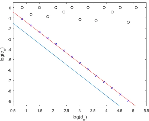
We will first look at the condition numbers of the roots of the Mandelbrot polynomials. As

mentioned in Chapter 1, the condition number for the roots is 1/p0

n(z). Figure 2.1 shows

the log-log plot of both the minimum and maximum condition numbers against the degree

of the Mandelbrot polynomials. Here, the circles represent the maximum condition numbers,

in which the minimum p

0

n(ξn)

, whereξnis a root of pn(z), were used to compute our condition

numbers. It can be seen that none of the condition numbers here exceed the value of 1. On

the other hand, the crosses are the minimum condition numbers. Looking at the line of best fit

running through these data points, some roots become better conditioned as the degree of the

polynomials increase. The slope of this line is around−2 (the lower line with a slope of−2 is

there for reference).

Figure 2.1: Plot of both mininum and maximum condition numbers against degree of the Mandelbrot polynomials.

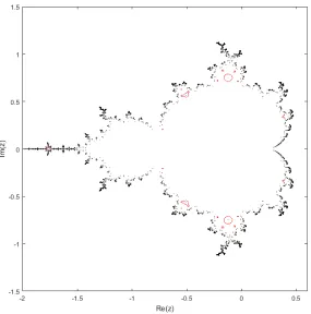
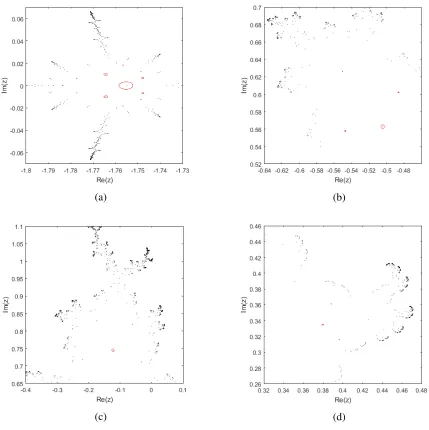
We can also plot the pseudozeros of the Mandelbrot polynomials by the plotting the

con-tours of pn(z) = ε, where εis an arbitrarily small number. Figure 2.2 illustrates this idea: it

(20)

2.3. Mandelbrot matrices 13

Figure 2.2: Roots ofp15(z) with|p15(z)|= 0.1 in red.

roots are too small to be seen, meaning that these roots are well-conditioned. However, the

roots in which the contours that surrounds it can be seen are those roots that are not as

well-conditioned. Figure 2.3 shows |p15(z)| = ε, where ε = 0.01, in red, at the most interesting

parts of the Mandelbrot polynomials, where the contours can be seen in Figure 2.2, but has the

contour|p15(z)|= 0.01 plotted instead.

Knowing that the roots are well-conditioned, we can now look at two different methods in

solving the Mandelbrot polynomials: an eigenvalue method and a homotopy method.

2.3 Mandelbrot matrices

The Mandelbrot matrices, first thought of by Piers Lawrence [9], are recursively-constructed

(21)

(a) (b)

(c) (d)

(22)

the corresponding Mandelbrot polynomials. We begin our recursive matrices with

M2 =

−1

, (2.9)

which corresponds to p2(z). It is obvious that the eigenvalue of Equation (2.9) is−1, which is

clearly the root of p2(z)= z+1. Letrn =

0 0 . . . 1

andcn=

1 0 · · · 0

T

, where

the length of both vectors aredn =2n−1−1. Then, our matrix construction is

Mn+1=                    

Mn −cnrn

−rn 0

−cn Mn                     ,

for alln>1. The first few Mandelbrot matrices are

M3=                    

−1 0 −1

−1 0 0

−1 −1

                    , (2.10) and

M4 =                                                       

−1 0 −1 −1

−1 0 0

−1 −1

−1

−1 −1 0 −1

−1 0 0

−1 −1

                                                       . (2.11)

Evaluating the eigenvalues of both M3 andM4, we can see that the eigenvalues are the roots

of p3(z) and p4(z) respectively. We can show that pn(z) = det(zI− Mn) for alln > 0 using

(23)

Figure 2.4: All 32,767 roots ofp16(z), produced in Maple 2016.

2.3.1 Using full matrices

Using Maple 2015, we were able to compute up to n = 16, which is 32,767 roots using a

machine with 32 GB of memory, shown in Figure 2.4. Although the Mandelbrot matrices are

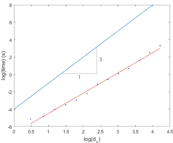
sparse, initially, for simplicity’s sake, we used full matrices in our eigenvalue computation.

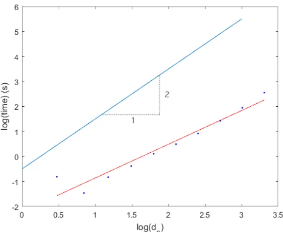
Figure 2.5 shows the time taken to compute the eigenvalues of the Mandelbrot matrices as the

dimensiondnof the matrix increases. As you can see from the figure, the line fitted to the data

(the bottom red line) is not as steep as the reference line (the top line), which has a slope of 3.

In fact, the slope of the line of fit is around 2.3. Therefore, this method has a time complexity

of order less than O(dn3). This fact is surprising because we expected this method to have a

time complexity of exactlyO(d3

n). We believe that the time complexity calculated here is less

than what we expected because the algorithm effectively uses a divide and conquer approach

to solve for the eigenvalues due to the structure of these companion matrices, thus reducing the

(24)

breaking into roughly equal halves.

Figure 2.5: Time taken for eigenvalue computation of Mandelbrot matrices. The slope of the line of best fit is around 2.3.

Since we are using full matrices in our eigenvalue computations, this means that the space

complexity is quite large, O(d2n), and since the matrices that we are working with are quite

sparse, most of the numbers that are stored would actually be zeros. Therefore, using the

sparse data type would help us save space when storing our matrices, and hopefully help us

compute more roots. However, computing eigenvalues using sparse data structures do present

some difficulties which will be discussed in the next subsection.

2.3.2 Using sparse matrices

To take advantage of the sparseness of the matrices when solving for the eigenvalues, we can

use MATLAB’s eigs routine, which uses Arnoldi iteration to solve for eigenvalues. Unlike solving for eigenvalues using full matrices, we cannot solve for all of the eigenvalues at once.

Instead, we have to look at different regions and compute the eigenvalues that are in each region

(25)

trying to find all of the eigenvalues of the Mandelbrot matrices.

The first issue is determining what regions to look at that would help us compute our

eigen-values. Borrowing the idea from homotopy methods (which will be discussed later in this

chapter), we can use the roots from the previous iteration to help us locate the new roots.

How-ever, for matrices of higher dimensions, it becomes increasingly difficult to locate all of the

eigenvalues. Therefore, as the dimension of the matrices increases, the number of

eigenval-ues that need to be found at each region also increases. Also, since we are computing several

eigenvalues from each region, it means that we will end up getting duplicates. This introduces

another challenge of eliminating all of the duplicate eigenvalues that were computed, so that

each eigenvalue only appears once. Since these eigenvalues are computed numerically, the

eigenvalue duplicates may not necessarily be exactly the same. This imposes another

chal-lenge when comparing two results in determining whether they are in fact duplicates of each

other or whether they are distinct roots, but located near each other. Unfortunately, using this

routine, we were only able to compute all of the roots up ton=13, which is only 4,095 roots.

In the interest of time, we decided not to pursue this any further.

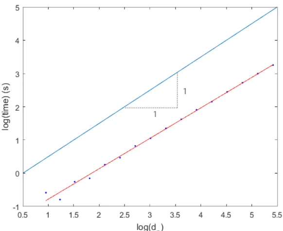
The time taken to compute these eigenvalues of the Mandelbrot polynomials using sparse

matrices can be seen in Figure 2.6. The slope of the line that passes through the data points is

around 1.3; the line above it is a reference for the steepness of a slope of 2. Although, here,

it shows that the time complexity is of order O(d1n.3), which is less than the time complexity

when using full matrices, it does not seem quite correct. However, we are lacking some data

since we are only considering the time computed for up ton= 13. Once higher dimensions are

achieved using this method, the time complexity may increase; it might possibly have a higher

time complexity than the method that uses full matrices. Therefore, more research would need

(26)

2.4. Homotopy method 19

Figure 2.6: Time taken for eigenvalue computation using sparse matrices. The slope of the line of best fit is around 1.3.

2.4 Homotopy method

Consider this special-purpose homotopy

Hn(ζ, τ)= ζ(pn−1(ζ))2+τ2. (2.12)

When τ = 0, it is clear that the zeros of the homotopy is ζ = 0, and the zeros (twice) of

pn−1(z), which, in other words, are the rootsξn−1 of the previous polynomials. On the other

hand, whenτ = 1, Hn(ζ, τ) is the same as our Mandelbrot polynomials, which means that the

roots of our homotopy are equivalent to the roots of pn(z). Therefore, by differentiating both

(27)

describes a path from the roots ofζ(pn−1(ζ))2 to the roots ofpn(ζ), provided thatp0n(ζ),0:

0= Hn(ζ, τ)

0= d

dτHn(ζ, τ)

= dζ

dτ· p

2

n−1(ζ)+2ζ· pn−1(ζ)·p0n−1(ζ)

dζ dτ+2τ

= dζ

dτ

p2_n−1(ζ)+2ζpn−1(ζ)

+2τ

= p0n(ζ)

dζ

dτ+2τ . (2.13)

Thus,

dζ dτ = −

2τ

p0

n(ζ)

, τ∈[0,1]. (2.14)

However, since our initial conditions include the roots of the previous polynomial,ξn−1, it

means that we encounter a singularity when we first solve this differential equation numerically.

To reiterate,p0_n(z)= pn−1(z)(pn−1(z)+2zp0n−1(z)), and sinceξn−1is a double root ofzp 2

n−1(z), this

means that p0_n(ξn−1)= 0. Additionally, sinceξn−1is a double root, this also means that two new

rootsξn will stem from this one initial condition. In order to achieve this, we can use Taylor

series expansion to perturb our initial conditions so that our solutions will go on two different

paths, thus giving us two distinct solutions for each previous root. Letζ = ξn−1+aτ+O(τ2),

whereτis arbitrarily small. To find what the coefficientais, we can do the following:

pn−1(ζ)= pn−1(ξn−1+aτ)

pn−1(ξn−1+aτ)= pn−1(ξn−1)+aτp0n−1(ξn−1)+O(τ2)

pn−1(ξn−1+aτ)=aτp0n−1(ξn−1)+O(τ2). (2.15)

Substituting this into the right hand side of Equation (2.12) and setting this expression to 0, we

get the following:

0= (ξn−1+aτ)(aτp

0

(28)

2.4. Homotopy method 21

From here, we can collect the coefficients of powers of 2 forτ, and solve fora, which is

a=± 1

p0

n−1(ξn−1) s

−1 ξn−1

. (2.17)

As we can see from Equation (2.17),acan either be positive or negative. This means that we

can perturb our initial conditions in two different directions. Instead of using

ζ(0)= ξn−1, (2.18)

as our initial condition, we would use

ζ(τ)=ξn−1+

τ

p0_n₋₁(ξn−1) s

−1 ξn−1

(2.19)

and

ζ(τ)=ξn−1−

τ

p0

n−1(ξn−1) s

−1 ξn−1

, (2.20)

resulting in finding two different roots. Therefore, using this technique, we are able to perturb

our initial condition, ξn−1, to avoid the singularity that we encounter when τ = 0. This is

essentially the Puiseux expansion ofζ(τ):

ζ(τ)= ξn−1±aτ+O(τ2) (2.21)

and the reason we usedτ2 _{instead of just simply}_τ_{in the homotopy.}

Unfortunately, these are not the only singularities that we encounter when solving Equation

(2.14). As an example, we can look at the singularities that we encounter when n = 3. The

differential equation for p3(z) is

dζ dτ =

−2τ

3ζ2+₄ζ+₁ , (2.22)

(29)

that we will encounter singularities whenζ(τ)= −1 and−1₃, which is whenτ 0.3849. This

will give us problems when trying to integrate along the realτ-axis. Therefore, we need to use

some method, such as the pole-vaulting technique, in order to avoid these singularities.

2.5 Pole-Vaulting

The pole-vaulting technique is a way to avoid singularities by backing offfrom the pole slightly,

and then going in a semicircular arc in the complex τ-plane (see [8, Section 12.11.1]), also

visually shown in Figure 2.7. Our semicircular path can be defined as

τ= p−ρeiθ, (2.23)

where pis the location of our singularity (which is a pole), andρis the radius of our

semicir-cular arc (or mathematically,ρ = p−τ). From Equation (2.23), we can see that whenθ = 0,

τ = p−ρ, and whenθ = π, τ = p+ρ. This means that we will be hopping over the pole by

taking 0≤ θ≤π.

τ=0 x 1

p

ρ

Figure 2.7: Diagram demonstrating pole-vaulting technique (pis the pole, andρis the radius of the semicircular arc).

Therefore, our ordinary differential equation for pole-vaulting becomes

dζ dθ =

dζ dτ

dτ dθ =

−2i(p−ρeiθ)ρe−iθ p0

n(ζ)

, θ∈[0, π]. (2.24)

Using this pole-vaulting technique, we can easily integrate Equation (2.22). Figure 2.8 shows

the paths (in black) that were taken to achieve the roots for p3(z). In the figure, the blue circles

(30)

2.5. Pole-Vaulting 23

grey line is the contour|p3(ζ)|= 1. Notice that in this figure, two of the final roots stem from

our initial pointζ =ξ2 = −1, and only one root comes fromζ = 0. This matches our previous

comment about needing to perturb our initial conditions so that we can get two separate paths

from this initial point. Figure 2.9 shows the homotopy paths of the Mandelbrot polynomials

fromn= 4 ton=9.

Figure 2.8: Homotopy paths ofp3(z) and contour where|p3(z)|= 1.

2.5.1 Residues

Our discussion about pole-vaulting thus far only looks at the case where we are integrating in

a semi-circular arc above the real axis. However, we are also interested in knowing whether

integrating along a semi-circular path below the real-axis would give us the same result. To

determine whether there is any difference, we can compute the residues by integrating around

(31)

(a) n=4 (b) n=5

(c) n=6 (d) n=7

(e) n=8 (f) n=9

Figure 2.9: Plots of homotopy paths and contour |pn(z)| = 1 of the Mandelbrot polynomials

(32)

2.5. Pole-Vaulting 25

when θ = 2π. In MATLAB, using our own ode solver (which will be discussed later in this

chapter), the residues are of orderO(10−2). Since this value is much smaller than the distance from where we start integrating our differential equation in the complex plane to our pole, we

believe that it does not matter whether we use a pole-vaulting technique to integrate above or

below the real axis. We also used multiple precision to compute the residues to ensure that

the values that we computed for our residues were just simply due to the numerical technique

that was used. The residues computed with higher precision areO(10−5_{), which is less than the}

value that we computed when using MATLAB, as expected. Therefore, this confirms that we

should be able to compute all of the roots of the Mandelbrot polynomials regardless of whether

we are integrating above or below the real axis.

2.5.2 Distinctness

From the paper [10], we learn that all of the roots in this family of polynomials are distinct.

To ensure that this statement is true, we need to make sure that the paths of integration of all

routes taken to find the roots do not cross, thus leading us to find all the roots without getting

any duplicates. To illustrate this, we can see that none of the homotopy paths cross in each

plot of Figure 2.9. However, this is not a strong enough argument to confirm that all paths

are distinct. We also need to prove uniqueness, which requires the Lipschitz condition in a

domain R to be satisfied in order for there to be at most one solution [5, Chapter 6.3]. We,

however, already know that the solutions of the differential equations are not unique if our

initial condition is ζ(0) = ξn−1, since it is a double root. Therefore, in place of ζ(0) = ξn−1

as our initial conditions, we will use our perturbed initial conditions (see Equations (2.19) and

(2.20)).

Consider the following general initial value problem:

(33)

We say that f satisfies a Lipschitz condition in a region R if there is a constant L ≥ 0 such

that [5, Chapter 6.2]

|f(t,u)− f(t,v)| ≤ L|u−v|, if (t,u), (t,v)∈ R. (2.26)

Letting our regionR= _C∼S, whereS is a small region surrounding each singularity, and

applying this definition to our homotopy for the Mandelbrot polynomials,

|f(t,u)− f(t,v)| ≤L|u−v|=

−2t p0

n(u)

− −2t

p0

n(v) =

−2t p0_n(v)− p0_n(u)

p0

n(u)p0n(v) . (2.27) Defining

p0n(v)= p

0

n(u+v−u)

= p0_n(u)+ p00_n(u)(v−u)+O(v−u), (2.28) we get

L|u−v|=

−2t p0n(u)+ p

00

n(u)(v−u)+O(v−u)

p0

n(u)p0n(v)

−2t p00n(u)

p0

n(u)p0n(v)

|v−u| . (2.29)

Therefore,

L= −2t p

00

n(u)

p0

n(u)p0n(v)

. (2.30)

However, sincep0n(u)≈ p

0

n(v), we can rewrite Equation (2.30) as

L= −2t p

00

n(u)

(p0

n(u))2

(34)

2.6. Our custom ode solver 27

As long as we avoid the singularities, when p0n(z)=0, we will be following a continuous path,

which means that the second derivative is bounded. From this, we know thatLis also bounded,

thus satisfying the Lipschitz condition. Therefore, this shows that the solutions to our initial

value problems are in fact unique.

2.6 Our custom ode solver

When we first started, we used MATLAB’s ode45routine to solve our differential equations to find the roots of the Mandelbrot polynomials. However, instead of using the pole-vaulting

technique, we decided to integrate in the complex plane using a triangular pathway. We were

able to compute all of the roots up ton = 20, which is 524,288 roots, until some pathways

diverged offto infinity when computing some of the roots whenn = 21, due to the increased

density of the singularities. Therefore, we decided to write our own ode solver in MATLAB

(and eventually in C++) to solve these differential equations so that we can step around the

roots by using pole-vaulting. Although we could have used MATLAB’s ode45 routine for

the pole-vaulting technique, we did not want to compute all of the singularities as it becomes

computationally expensive for high degrees. Therefore, our ode solver is based on MATLAB’s

ode45routine, which uses the Runge-Kutta-Fehlberg algorithm, but instead of terminating the program when it reaches a singularity, it is able to step around the singularity using the pole

vaulting technique described in the previous section and continue integrating until it reaches

the final point, which in our case isτ=1.

2.6.1 Runge-Kutta Methods

Euler’s method is the simplest method for solving an ordinary differential equation numerically.

However, it is not very accurate (or at least not accurate enough for our liking) since it is only

a first order method. To improve on this, we could use Taylor series expansion to increase the

order of our solution by using higher order derivatives. Since p0n(z), p

00

(35)

approximations are also available in O(n), i.e. O(lndn), flops, Taylor series methods could

well be viable for this problem. However, we decided to take another approach: to evaluate

the derivative function f(t,x(t)) more than once at different points, and then use a weighted

average of the values thus obtaining an approximation of the slope of the secant. This idea

gives what are called the Runge-Kutta (RK) methods, which we have found to be adequate for

our needs.

There are different RK methods in use [8, Chapter 13]. If we let the weights bebi, the time

step beh, andi=1,2,3, . . . ,s, the general form for an explicit Runge-Kutta methods is

xk+1= x0+h(b1k1+· · ·+bsks)= xk+h s X

i=1

biki, (2.32)

where the stages are

k1 =f(tk,xk)

k2 =f(tk+c2h,xk+a21k1)

k3 =f(tk+c3h,xk+a31k1+a32k2)

...

ks=f tk +csh,xk +as1k1+as2k2+· · ·+as,s−1ks−1 , (2.33)

which can also be expressed as

ki =f        

tk +cih,xk +h i−1 X

j=1

ai jkj        

, (2.34)

Here, the ci andai j are the weights of our previously computed values of kj, j < i. We can

(36)

2.6. Our custom ode solver 29

the following form:

c A

bT

=

0

c2 a21

c3 a31 a32

... ... ... ...

cs as1 as2 · · · as,s−1

b1 b2 · · · bs−1 bs

, (2.35)

whereAis a lower-triangular matrix with zeros as diagonal entries.

For robustness and to ensure quality of the solution, we need an adaptive step size scheme.

The goal of an adaptive step scheme is to take the largest stepsize possible while ensuring that

the absolute local truncation error is less than a tolerance given by the user for every step.

Here, we have decided to use the Runge-Kutta-Fehlberg method (RKF45) [12], which is a

fourth-order method with an error estimate of orderO(h5). TheButcher tableaufor the

Runge-Kutta-Fehlberg method, where the first row of coefficients at the bottom of the table gives the

fifth-order accurate method, and the last row gives the fourth-order accurate method, is

0

1/4 1/4

3/8 3/32 9/32

12/13 1932/2197 −7200/2197 7296/2197

1 439/216 −8 3680/513 −845/4104

1/2 −8/27 2 −3544/2565 1859/4104 −11/40

16/135 0 6656/12825 28561/56430 −9/50 2/55

25/216 0 1408/2565 2197/4104 −1/5 0

(37)

From Equation (2.36), we can see that the fourth-order approximation is

xi+1= xi+

25 216k1+

1408 2565k3+

2197 4104k4−

1

5k5 (2.37)

and our fifth-order approximation is

˜xi+1 =xi+

16 135k1+

6656 12825k3+

28561 56430k4−

9 50k5+

2

55k6. (2.38)

The local truncation error is

τi+1= ˜xi+1−xi+1. (2.39)

We can use the truncation error to help us calculate the size of the next step. By Taylor’s

theorem, our local truncation error is proportional to

τi+1 =khp+1 (2.40)

for some constantkand where p, in our case, is 4. So, we can multiply a scalarqwithhto get

the following:

τi+1(qh)=kqphp

=qpkhp

=qpτi+1(h)

≈qp(˜xi+1−xi+1) . (2.41)

Therefore, to make

|τi+1(qh)| ≈ |qp(˜xi+1−xi+1)|<tol, (2.42)

we want

q≤

"

tol |˜xi+1−xi+1|

#1/p

(38)

2.7. Accuracy of the roots 31

but in practice, we use

q≤ 0.8

"

tol |˜xi+1−xi+1|

#1/p

. (2.44)

Therefore, the optimal step size for the next step isqh. This is a very primitive way of step-size

control, but has worked adequately for these problems, most notably because we may improve

the approximate answer by a Newton step on pn(z)= 0.

We can take advantage of the automation of the step sizes to help us locate singularities

that are in the way. In our ode solver, once the step size falls below a certain size, say 10−6, the method will start integrating around the singularity using the Runge-Kutta-Fehlberg method

once again. As a reminder, the differential equation that is used to integrate around the

singu-larity is given as

dζ dθ =

dζ dτ

dτ dθ =

−2i(p−ρeiθ)ρe−iθ p0

n(ζ)

, θ∈[0, π],

which can also be found as Equation (2.24). The problem that we encounter here is that we

actually do not know what p or ρ are since we do not know where the exact location of the

singularities are. Therefore, to estimateρ, which is the distance that we are from the pole, we

can use Newton’s method

ρ= ζi−

p0n(ζi)

p00

n(ζi)

, (2.45)

since the denominator of our differential equation is just simply p0

n(ζ), and we can easily

cal-culate p0

n(ζi) and p00n(ζi).

Once the semi-circular path is finished integrating (whenθ = π), our ode solver continues

integrating along its original path until it reachesτ=1.

2.7 Accuracy of the roots

To check for the accuracy of these roots, we can calculate the residuals by evaluating pn(ξn).

We expect that we can use Newton’s method to reduce the size of the residuals of each of the

(39)

2.7.1 Newton polishing

To improve on the accuracy of our roots, we expect that we can use Newton’s method to polish

the roots:

ξn= ξn−

pn(ξn)

p0

n(ξn)

. (2.46)

We only polish each root once as we fear polishing the roots any more than that may cause the

roots to skip over to another root. However, Newton’s method may not actually give us better

results. As we can see from the paper [10] by Corless and Lawrence, Newton’s method has

problems when p00n(z) is too large, which the authors found out when trying to find the largest

roots of the Mandelbrot polynomials.

The authors began with the observation that the largest root is quite close to, but slightly

closer to zero than,−2. In order to use Newton’s method, the derivatives need to be calculated,

which they found to be (atz=−2)

p0n(z)=

4n−1₋₁

3 , (2.47)

which resulted in the Newton estimate to be

zn −2+

3

4n−1₋₁. (2.48)

However, the Newton estimate above is not quite right: the error of Equation (2.48) isO(4−n_),

but the guess is alreadyO(4−n_{) accurate, so taking a Newton step hardly improves this estimate.}

Therefore, we need to look at the growth of higher derivatives. The Newton estimate is based

on the expansion

pn(−2+ε)= pn(−2)+ p0n(−2)ε+

1 2p

00

n(−2)ε

2₊_{· · ·} _, _(2.49)

(40)

2.8. Smallest roots 33

second derivative of the Mandelbrot polynomial evaluated at−2 is

p00_n(−2)=− 1 274

2n₊ 1

3−

k

9

!

4n− 8

27 , (2.50)

which exposes the problem with Newton’s method. Here, p00n(−2) is O(ε

−2_{), so we cannot}

neglect theO(ε2) term in this case. In [10], the authors go on to find an analytical expression

for the largest magnitude real roots of the Mandelbrot polynomials, but we shall not need that

here.

2.8 Smallest roots

We can also use homotopy methods, as described above, to find the smallest roots, sn, of the

Mandelbrot polynomials by just simply using the smallest root from the previous iteration as

our starting point. We empirically deduce from our computations that thatsn has the form:

sn =

1

4 +αRen

−βRe_±_iα

Imn−βIm+h.o.t. (2.51)

We can plot the real (minus 1/4) and imaginary part of the smallest roots in a log-log plot,

shown in Figure 2.10 to compute βRe and βIm, which turn out to be, to the accuracy that we

use, 2 and 3 respectively. However, we are not sure that these are exact. Therefore, we can

approximate

sn

1 4 +

αRe

n2 ±

αIm

n3 . (2.52)

Knowing what βRe andβIm are, we can computeαRe andαIm, which are approximately 9.869

and 58.81, respectively. Corless and Lawrence [10] conjectured thatαRe isπ2. This work does

(41)

(a) Real part (b) Imaginary part

Figure 2.10: Log-log plots of smallest roots sn of Mandelbrot polynomials (difference from

1/4)

2.9 Results for homotopy methods

We were able to compute in MATLAB, using our own ode solver, all the roots of the

Man-delbrot polynomials up to n = 22, which has a degree of 2,097,151 to the order of O(10−4₎

precision (see Figure 2.12). However, according to Bini’s personal website, they were able to

solve for around 4 million roots, which is one more iteration that what we have computed.

The time that it took to compute the roots using a homotopy method can be seen in Figure

2.11. In this figure, the line of best fit that runs through the data points has a slope of around

0.92, which is less than 1 (the line above our data is a reference to show the steepness of a line

with a slope of 1). Computationally speaking, this does not make any sense. There is a lower

bound on the complexity of O(dn) because we have to output dn roots; further, evaluating a

residual at each root costsO(lndn) flops, making an overall lower bound of O(dnlndn). What

must be happening here is that the “constant” hidden by theOsymbol is larger for the first few

n, and only is asymptotically constant. The roots are getting easier to find for largerdn.

As we compute the roots using our custom ode solver in MATLAB, we notice that we lose

accuracy as the iteration increases. We believe that the residuals are getting larger because of

the mild instability of the recurrence relation. Therefore, we need to use multiple precision in

(42)

2.9. Results for homotopy methods 35

for arbitrary precision in C++. Unfortunately, the ARPREC package does not lend itself to

OpenMP parallelization since it is not entirely thread safe [1]. Despite this, we were able to

compute up ton= 19, which has a degree of 262,143 thus far with the maximum residual of

O(10−11_).

(43)

Figure 2.12: All 2,097,151 roots of the Mandelbrot polynomial p22(z). These roots were

(44)

Chapter 3 Fibonacci-Mandelbrot polynomials and

matrices

3.1 Introduction

The Fibonacci sequence, which is Sequence A000045 of the Online Encyclopedia of Integer

Sequences [22] is a widely known sequence. It begins

0,1,1,2,3,5,8,13,21,34,55, . . . (3.1)

and is generated by the recursion

Fn= Fn−1+Fn−2 (3.2)

withF0 =0 and F1 =1. There is a plethora of resources such as [16], [18], and the references

therein, that talk about the Fibonacci sequence which can be referred to if the reader wants to

learn more about the Fibonacci sequence.

(45)

3.1.1 Fibonacci-Mandelbrot polynomials

The Fibonacci-Mandelbrot polynomials are very similar to the Mandelbrot polynomials,

de-scribed in the previous chapter, but are slightly different. As a reminder, the recursion for the

Mandelbrot polynomials is

pn+1(z)= zp2n+1, (3.3)

where p0= 0. The Fibonacci-Mandelbrot polynomials, on the other hand, have the recursion

q0(z)=0, q1(z)=1

qn+1(z)=zqn(z)qn−1(z)+1, (3.4)

wheren=1,2,3, . . .. Instead of taking the polynomial from the previous iteration and squaring

it, we are multiplying the polynomials from the previous two iterations together. This is the

reason why it is called the Fibonacci-Mandelbrot polynomials.

Expanding Equation (3.4) using the monomial basis expansion, we can get the first few

polynomials:

q0(z)=0

q1(z)=1

q2(z)=1

q3(z)=z+1

q4(z)=z2+z+1

q5(z)=z4+2z3+2z2+z+1

q6(z)=z7+3z6+5z5+5z4+4z3+2z2+z+1

q7(z)=z12+5z11+13z10+22z9+28z8+28z7+23z6+16z5+10z4+5z3+2z2+z+1.

(46)

3.2. Condition numbers and pseudozeros 39

Some properties of the Fibonacci-Mandelbrot polynomials include:

1. The leading and trailing coefficients are 1.

2. All coefficients are positive integers.

3. The polynomials are unimodular.

4. The next-to-leading coefficient is a Fibonacci number.

5. Putdn = degqn. Thend1 =0, d2= 0,dn+1 =dn+dn−1+1 ordn = Fn−1, whereFnis a

Fibonacci number (see Equation (3.2)).

6. The roots ofqn(z) lead to periodic points ofqn+1(z)=zqn(z)qn−1+1, of periodn−2. For

instance,q3(−1)=0,q4(−1)=1,q5(−1)= 1, and then repeats: qn(−1)={0,1,1}.

7. The coefficients ofqngrow doubly exponentially:O(φφ

n

),φ= 1+

√

5

2 1.618. . ..

3.2 Condition numbers and pseudozeros

Similar to the Mandelbrot polynomials, the absolute condition number of the roots is 1/q0n(z).

Figure 3.1 shows the minimum and maximum condition numbers of the roots of the

Fibonacci-Mandelbrot polynomials. The maximum condition numbers are represented by the circles, and

are computed by taking the reciprocal of the minimum value of q

0

n(z)

. On the other hand, the

minimum condition numbers are represented by the crosses, and computed by taking the

recip-rocal of the maximum value of q

0

n(z)

. Just as we have seen for the Mandelbrot polynomials,

the maximum condition number for the Fibonacci-Mandelbrot polynomials is also 1, which

means that the roots are well-conditioned. The slope for the line of best fit for the minimum

condition number for the Fibonacci-Mandelbrot polynomials is around−1.9, which is slightly

greater than−2. The line that is below the lines of best fit is for reference; it has a slope of−2.

Additionally, we can look at the pseudozeros of the Fibonacci-Mandelbrot polynomials by

(47)

Figure 3.1: Minimum and maximum condition numbers of the roots for Fibonacci-Mandelbrot polynomials.

with respect to the location of the roots. Figure 3.2 shows the roots ofq15(z) with the contours

of|q15(z)| = 0.2 in red. Here, we can see that the contours that are visible encircles the roots

quite closely, which mean that the roots are well-conditioned. We can look closer into some

of the more interesting regions (that contain more red) of the roots of Fibonacci-Mandelbrot

polynomials, and reduce the size of the contour that we are looking into for these particular

regions. In Figure 3.3, we zoom into 4 different regions of the roots of q15(z), and plotted

|q15(z)|=0.05 instead of|q15(z)|= 0.2.

3.3 Fibonacci-Mandelbrot matrices

Using Piers Lawrence’s idea of using supersparse companion matrices to compute the roots

(48)

3.3. Fibonacci-Mandelbrot matrices 41

(49)

(a) (b)

(c) (d)

(50)

Fibonacci-Mandelbrot polynomials,qn(z). We start with

M3= [−1], (3.6)

in which the eigenvalue,−1, is the root ofq3(z)= z+1 and

M4 =            0 1

−1 −1

           , (3.7)

where the eigenvalues,−1 2 ±

√

3i

2 , are the roots ofq4(z)=z

2₊_z₊_{1. Also, note that}

MT₄ =

          

0 −1

1 −1

           (3.8)

also leads to a similar family. However, we decided to use Equation (3.7) so that the

subdiago-nal of these family of companion matrices will always be−1.

Letrn =

0 0 · · · 1

andcn=

1 0 · · · 0

T

be row and column vectors of length

dn, wherednis the degree of the polynomial,qn(z). Then, our matrix construction would be

Mn+1 =                    

Mn (−1)dn+1cnrn−1

−rn 0

−cn−1 Mn−1                     (3.9)

for alln>2. The first few Fibonacci-Mandelbrot matrices are

M5 =                             

0 1 1

−1 −1

−1

−1 −1

(51)

and

M6 =                                                       

0 1 0 1 −1

−1 −1 0 0

−1 0 0

−1 −1

−1

−1 0 1

−1 −1

                                                       . (3.11)

Computing the characteristic polynomials for both Equations (3.10) and (3.11), they both

match the Fibonacci-Mandelbrot polynomials, q5(z) andq6(z), respectively. We can also

con-struct the Fibonacci-Mandelbrot matrices slightly differently: we can swapMn andMn−1, and

changernandcnto the correct lengths. Thus, the recursion for this companion matrix is

Mn+1 =                    

Mn−1 (−1)dn+1cn−1rn

−rn−1 0

−cn Mn

                    , (3.12)

(52)

ma-3.3. Fibonacci-Mandelbrot matrices 45

trices using the recursion shown in Equation (3.12) are

M5 =                             

−1 1

−1

−1 0 1

−1 −1

                             , (3.13)

M6 =                                                       

0 1 −1

−1 −1

−1

−1 −1 0 0 1

−1 0 0 0

−1 0 1

−1 −1

                                                       , (3.14)

in which the characteristic polynomials of bothM5(Equation (3.13)) andM6(Equation (3.14))

also matchq5(z) andq6(z) respectively. It can be shown thatqn(z)= det(zI−Mn) for alln> 3

using induction and the Schur complement [24], which will be shown in Chapter 5.

Unlike the Mandelbrot matrices, notice that the Fibonacci-Mandelbrot matrices contain

{−1,0,1}, whereas the Mandelbrot matrices contain just the values{0,−1}. What is also

inter-esting is that the inverses of these Fibonacci-Mandelbrot companion matrices have inverses that

(53)

M6(Equation (3.11)) that follows the recursion found in Equation (3.9),

M−₆1 =

                                                      

0 −1 1 0 0 0 0

0 0 −1 0 0 0 0

−1 0 −1 −1 1 0 0

0 0 0 0 −1 0 0

−1 0 −1 0 0 −1 0

1 0 1 0 0 0 −1

−1 0 −1 0 0 0 0

                                                       . (3.15)

We can also use Maple to help us visualize the next few inverses, shown in Figure 3.4, where

−1 is black, 0 is grey, and 1 is white. It is obvious from these plots that there is clearly a pattern

for the inverses of the Fibonacci-Mandelbrot polynomials. More research is required to learn

more about the inverses of these companion matrices and will be left to future work.

3.3.1 Results

Using our first matrix construction (Equation (3.9)), MATLAB’seigroutine was able to com-pute the eigenvalues of M22, which has a dimension of 17,710, correctly (see Figure 3.5a).

However, it was not able to successfully compute the roots ofq23(z) correctly, shown in

Fig-ure 3.5b. In MATLAB’s eigroutine, the default for balanceOption is ‘balance’, which enables balancing. In most cases, the balancing step improves the conditioning of the matrix

to produce more accurate results. However, in our case, it did not give us the correct results.

Therefore, we computed the eigenvalues once again with ‘nobalance’, but unfortunately, produced the same (incorrect) results. Additionally, we did not attempt to solve for the

eigen-values of sparse matrices even though it is very likely that it can help us find more roots using

this method.

We also tried computing the eigenvalues of the Fibonacci-Mandelbrot matrices using both

(54)

(a)M−1

7 (b)M

−1 8

(c)M−₉1 (d)M−₁₀1

(55)

(a) Computed eigenvalues ofM22, which has a

di-mension of 17,710.

(b) Computed eigenvalues computed of M23,

which has a dimension of 28,656.

Figure 3.5: Plots of eigenvalues using MATLAB’seigroutine.

results. Maple 2015 actually gives us the results that we were expecting (see Figure3.6a),

whereas Maple 2016 gives us inaccurate results (see Figure 3.6b).

From Figure 3.7, we can see that the time complexity is around O(dn2.3), which is very

similar to the time complexity that we computed when using the eigenvalue method on the

Mandelbrot matrices. As a reference, the top line has a slope of 3, which is the slope that we

expect our line of best fit to have.

3.4 Homotopy methods

We can also use homotopy methods to solve for the roots of the Fibonacci-Mandelbrot

poly-nomials. Consider the following homotopy:

Hn(ζ, τ)= ζqn−1(ζ)qn−2(ζ)+τ. (3.16)

Comparing this homotopy (Equation (3.16)) to the homotopy used for the Mandelbrot

(56)

3.4. Homotopy methods 49

(a) Using Maple 2015 (b) Using Maple 2016

Figure 3.6: Computed eigenvalues ofn = 23, which has a degree of 28,656 of the Fibonacci-Mandelbrot matrices using Maple.

(57)

is that the variableτin the homotopy for the Mandelbrot polynomials is squared, whereas here

in Equation (3.16), is just simplyτ. This is because the zeros whenτ= 0 are simple atζ = 0,

the roots ofqn−1(ζ), and the roots ofqn−2(ζ): we do not start at any double roots.

Similarly to the Mandelbrot polynomials, we can differentiate the right-hand side of

Equa-tion (3.16) with respect toτto give us the following differential equation:

dζ dτ =

−1

qn(ζ)

, (3.17)

where we integrate 0≤τ≤ 1. Just as we did for the homotopy method used for the Mandelbrot

polynomials, we can use the zeros ofζqn−1(ζ)qn−2(ζ) as our initial conditions to help us find

the roots ofqn(ζ).

Unfortunately, just as when solving the differential equations numerically for the

Mandel-brot polynomials, we encounter singularities along the real-axis when solving Equation (3.17)

for the Fibonacci-Mandelbrot polynomials. As an example for this case, we can look at the

singularities whenn= 4. The differential equation forq4(z) is

dζ dτ =

−1

2ζ+1, (3.18)

whereζ(0)= 0 andζ(0)= −1 (since it is the root ofq3(z)). There are no roots forq2(z), so we

do not includeq2(z) in our initial conditions. From Equation (3.18), it is obvious that we will

encounter a singularity whenζ = −1

2. Also, since Equation (3.18) is separable, we can easily

find the value ofτwhenζ =−1

2, and check thatτlies on the real-axis between 0 and 1.

dζ dτ =

−1 2ζ+1

(2ζ+1) dζ =−dτ

ζ2₊_ζ ₌₋_τ₊_C_, _where_C_{is a constant}_. _(3.19)

(58)

whenζ =−1 andτ=0, we can substitute the corresponding values to Equation (3.19):

(−1)2+(−1)=C

1−1=C

C= 0. (3.20)

Therefore, whenζ= −1 andτ= 0, our constantCis also 0. Knowing that our constantC = 0,

we can now solve forτwhenζ = −1

2 to see at what value ofτwe encounter a singularity for

Equation (3.18):

−1 2

!2 + −1

2

! =−τ

1 4 −

1 2 =−τ

−1 4 =−τ

τ= 1

4. (3.21)

This shows that we do in fact encounter a singularity if we integrate along the real-axis, which

means that we need to use the pole-vaulting technique described in the previous chapter (see

Section 2.5) in order to avoid the singularities.

Since we are not starting from double roots for the Fibonacci-Mandelbrot polynomials, this

means that we do not need to perturb our initial condition, which we had to do for the

Man-delbrot polynomials. Instead, we can simply use the zeros of ζqn−1(ζ)qn−2(ζ), as mentioned

before. This means we only will get one root from each initial condition, unlike in the

Man-delbrot polynomials, where we get 2 roots from the zeros of pn−1(ζ) (remember that we only

got 1 root fromζ =0 for the Mandelbrot polynomials). As demonstrated in Figure 3.8, created

in MATLAB, we can see the homotopy paths taken from our initial points to our roots,ξ5. In

this figure, the root, ξ3 = −1, is indicated by a triangle, the roots, ξ4 = −0.5± 0.86603. . .,

(59)

Figure 3.8: Homotopy paths forq5and contour where|q5(z)|=1.

The grey line that surround the roots is the contour,|q5(z)|= 1. Notice in this figure that three

singularities are avoided by pole-vaulting.

Figure 3.9 shows the homotopy paths of the Fibonacci-Mandelbrot polynomials fromn=6

to n = 11. To simplify the plots, all of the initial points are blue circles (instead of showing

where each initial point comes from), while the final points are red crosses. These plots clearly

show that only one root stems from each initial point, unlike the Mandelbrot polynomials, seen

in Figure 2.9. One can prove that the gcd of qn(z) and qn−1(z) is 1: they can have no roots in

common because each would be periodic with periodnandn−1 and hence a fixed point, but

(60)

(a) n=6 (b) n=7

(c) n=8 (d) n=9

(e) n=10 (f) n=11

Figure 3.9: Plots of homotopy paths and contours |qn(z)| = 1 of the Fibonacci-Mandelbrot

(61)

3.4.1 Distinctness

Just as we have seen with the homotopy paths for the Mandelbrot polynomials, the paths for

the Fibonacci-Mandelbrot polynomials also do not cross (see Figures 3.8 and 3.9). We can

also prove, just like in Section 2.5.2, that each initial value problem is unique as long as the

singularities are avoided. However, this time, we do not need to be concerned about the initial

condition, and can start with the zeros ofζqn−1(ζ)qn−2(ζ), since these are not double roots.

Just as we did for the Mandelbrot polynomials, letting our region R = _C, we can find the

Lipschitz constant for the homotopy for the Fibonacci-Mandelbrot polynomials

|f(t,u)− f(t,v)| ≤L|u−v|=

−1 q0

n(u)

− −1

q0

n(v) =

−q0n(v)+q

0

n(u)

q0

n(u)q0n(v) . (3.22) Let

q0_n(v)=q0_n(u+v−u)

=q0n(u)+q

00

n(u)(v−u)+O(v−u). (3.23)

Substituting Equation (3.23) into Equation (3.22), we get

L|u−v|=

−q0_n(u)−q00_n(u)(v−u)+q0_n(u)+O(v−u)

q0

n(u)q0n(v)

−q00_n(u)

q0

n(u)q0n(v)

|v−u|

−q00n(u)

(q0

n(u))2

|v−u| . (3.24)

Therefore,

L= −q

00

n(u)

(q0

n(u))2

. (3.25)

A comparison of solution methods for Mandelbrot-like polynomials

Scholarship@Western

Scholarship@Western

A comparison of solution methods for Mandelbrot-like

A comparison of solution methods for Mandelbrot-like

polynomials

polynomials

Abstract

Contents

List of Figures

Chapter 1

Introduction

1.1

Conditioning

1.2

Root-finding methods

Chapter 2

Mandelbrot polynomials and matrices

2.1

Mandelbrot polynomials

2.2

Condition numbers and pseudozeros

2.3

Mandelbrot matrices

2.3.1

Using full matrices

2.3.2

Using sparse matrices

2.4

Homotopy method

2.5

Pole-Vaulting

2.5.1

Residues

2.5.2

Distinctness

2.6

Our custom ode solver

2.6.1

Runge-Kutta Methods

2.7

Accuracy of the roots

2.7.1

Newton polishing

2.8

Smallest roots

2.9

Results for homotopy methods

Chapter 3

Fibonacci-Mandelbrot polynomials and

matrices

3.1

Introduction

3.1.1

Fibonacci-Mandelbrot polynomials

3.2

Condition numbers and pseudozeros

3.3

Fibonacci-Mandelbrot matrices

3.3.1

Results

3.4

Homotopy methods

3.4.1

Distinctness