2-D DOA Estimation of LFM Signals for UCA Based
on Time-Frequency Multiple Invariance ESPRIT
Kaibo Cui*, Weiwei Wu, Jingjian Huang, Xi Chen, and Naichang Yuan
Abstract—In order to improve the angle measurement precision with a low computational complexity, a 2-D direction of arrival (DOA) estimation algorithm UCA-TF-MI-ESPRIT is proposed in this paper. This algorithm is based on the mode space algorithm and the time-frequency (TF) multiple invariance rotational invariance technique (MI-ESPRIT). Firstly, a uniform circular array (UCA) is equivalent to a virtual uniform linear array (ULA) by utilizing mode-space algorithm. Then, the smoothed pseudo Wigner-Ville distribution (SPWVD) of the ULA output is calculated. The spatial time-frequency matrix can be obtained through the average of multiple time-frequency points in the time-frequency plane, and the signal subspace can also be obtained through using eigen decomposition. Then a simple and effective subarray dividing approach is proposed, and the multiple rotational invariant equation of the array is obtained by using the Bessel function. Finally, the closed-form solution is obtained using multi-least-squares (MLS) criterion so that the 2-D DOA estimation of LFM signals in UCA is completed. The simulation results verify the effectiveness of the algorithm proposed by this paper.
1. INTRODUCTION
Compared with a uniform linear array (ULA), a uniform circular array (UCA) has some congenital advantages in the field of direction of arrival (DOA) estimation, such as fewer array elements, two-dimensional (2-D) fuzzy direction finding, wide frequency range and simple installation structure [9]. So, it has been widely used, and the DOA estimation of UCA becomes an important issue nowadays [1– 5, 27–29]. In the field of direction finding, the methods based on egien-subspace have been getting lots of attention for the excellent estimation performance. These kinds of algorithms have been developed a lot in recent years, such as multiple signal classification (MUSIC) algorithm [6] and estimation of signal parameters via rotational invariance techniques (ESPRIT) algorithm [7, 8]. In terms of estimation precision, MUSIC algorithm has a significant advantage. But the algorithm needs spectral peak searching, and its high precision requires small angle search step which greatly increases its computational complexity. ESPRIT algorithm does not need to search the spectrum, so it owns a low computational complexity, and the algorithm is prone to be easily realized in engineering [9]. Through mode-space algorithm [10, 11], ESPRIT algorithm can also be applied to the UCA. The traditional ESPRIT algorithm takes advantage of only a single displacement invariance in the sensor array. There are many situations, however, where the array possesses several such invariances [12–14]. In order to make full use of the invariances of the array, [12] proposes multiple invariance ESPRIT (MI-ESPRIT) algorithm and obtains a perfect estimation performance. In [13], the authors propose a closed-form MI-ESPRIT algorithm and obtain the analytical solutions of the multiple rotational invariant equation using multi-least-squares (MLS) criterion and regularize (RLS) criterion, which reduces the computational complexity greatly.
Received 22 November 2016, Accepted 9 January 2017, Scheduled 26 January 2017 * Corresponding author: Kaibo Cui (sky [email protected]).
With the rapid development of signal processing technology, broadband signals have become the main choice for the detection equipment such as sonar and radar. Especially for the linear frequency modulation (LFM) signal, it has been widely used in many cases. So the DOA estimation of LFM signals becomes an important issue. However, as the LFM signal belongs to a typical non-stationary signal, the traditional subspace algorithms which are based on stationary signals cannot be applied to such conditions. The time-frequency (TF) analysis is an effective tool for processing non-stationary signals. It can transform the signal from time domain to two-dimensional time-frequency plane. Through this way, the signal owns both the time and frequency domain features at the same time, which can improve the signal to noise ratio (SNR). LFM signals possess ideal energy collection features in the time-frequency plane so that the time-frequency analysis tools are very suitable to process them [15]. So, a series of DOA estimation algorithms based on the time-frequency analysis tools have been developed [16– 26]. In [16–20], the authors propose DOA estimation algorithms based on Wigner-Ville distribution (WVD). They introduce the time-frequency analysis tools to the DOA estimation field and obtain perfect estimation results. In [21–26], the authors consider the estimation of DOA exploiting MUSIC or ESPRIT algorithms based on the spatial time-frequency distribution (STFD) and obtain a perfect estimation performance.
In order to improve the estimation precision and efficiency, this paper proposes UCA-TF-MI-ESPRIT algorithm which is a 2-D DOA estimation algorithm of LFM signals based on mode-space algorithm and time frequency MI-ESPRIT algorithm. Firstly, the UCA is equivalent to a virtual uniform linear array (ULA) via mode-space algorithm. As the smoothed pseudo Wigner-Ville distribution (SPWVD) can restrain the cross-term interferences of the standard WVD, we use SPWVD instead of WVD as the time-frequency analysis tool in this paper. Then the SPWVD of each element’s output of the ULA is calculated. The spatial time-frequency matrix can be obtained through the average of multiple time-frequency points in the time-frequency plane, and the signal subspace can also be obtained using Eigen decomposition. A simple and effective subarray dividing approach is also proposed in this paper, and the multiple rotational invariant equation of the array is obtained. Finally, the closed-form solution is obtained using MLS criterion. The UCA-TF-MI-ESPRIT algorithm can be applied to the UCA and realize 2-D DOA estimation of multiple LFM signals. This algorithm does not need to exceed two-dimensional spectral peak searching, so it owns a pretty low computational complexity. The estimation precision of the UCA-TF-MI-ESPRIT algorithm is superior to the traditional UCA-ESPRIT algorithm, UCA-MI-ESPRIT algorithm and UCA-TF-ESPRIT algorithm. The simulation results show the good performance of the algorithm proposed by this paper.
2. THE UCA DATA MODEL OF LFM SIGNALS
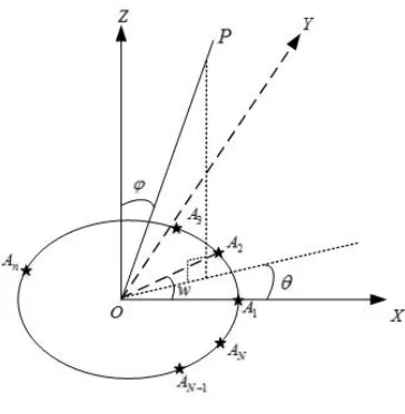
Considering a UCA with N elements, the array model is shown in Fig. 1. An(n = 1,2, . . . , N) is the element of the UCA. w is the angle between the array elements, so w = 2π/N. The far-field incident wave comes from P O. ϕ is the elevation angle of the incoming signal. θ is the azimuth angle of the incoming signal.
If there areM LFM signals from far field, the output of the array can be written as:
X=AS+N (1)
In Eq. (1), X = [ x1 x2 . . . xN ]T is a N × 1 output matrix of the array. S = [ s1 s2 . . . sM ]T is a M ×1 data matrix of far-field LFM signals. N = [ n1 n2 . . . nN ]T is a N×1 data matrix of noises which are additive white Gaussian noises, and the noises of each array element are not relevant. A= [ a1 a2 . . . aM ] is aN×M main fold vector matrix which satisfies:
ai = [ exp(−j2πfi(t)τ1i) . . . exp(−j2πfi(t)τNi) ]T (2)
fi(t) = fi+kit (3)
In Eq. (3), fi(t) is the instantaneous frequency of the ith signal at t. fi is the initial frequency of the ith signal. ki is the modulated frequency of the ith signal. In Eq. (2), τni is the time delay of the ith LFM signal on the nth element respect to the reference element. As the second-order term of
Figure 1. The UCA array model.
As the instantaneous frequencies of LFM signals change over time, the manifold vector of the array is time-varying for LFM signals.
If we regardO in Fig. 1 as a virtual reference element,
τni=rsinϕicos(θi−(n−1)w)/c (4) In Eq. (4), r is the UCA radius. c is the speed of light. θi is the azimuth angle of the ith LFM signal. ϕi is the elevation angle of the ith LFM signal.
3. UCA-TF-MI-ESPRIT ALGORITHM
3.1. Mode-Space Algorithm
Mode-space algorithm is a type of spectral estimation algorithm for the UCA, and its central idea is to equalize a UCA to a virtual ULA through mode excitation [10, 11]. Based on Eqs. (1) and (2), the output of thenth element can be written as:
xn= M
i=1
exp(−j2πfi(t)τni)si (5)
We can carry outN point discrete Fourier transform (DFT) forxn and get:
vm = N
n=1
xnexp(−j2πnm/N) = N
n=1 M
i=1
exp(−jβicos(θi−(n−1)w))siexp(−j2πnm/N)
≈N
M
i=1
j−mJ−m(−βi) exp(−jmθi)si (6)
m ∈[− β,β]∩Z, N >2β (7) In Eq. (6), Jm( ) stands for the mth order of Bessel function. βi = 2πrfi(t) sinϕi/c, β = max
i=1,2,...,M{2πrfi(t)/c}. is the rounded down symbol. Z is the mathematical set of all integers. If K = β, the phase modes excited by the UCA are: −K,−K + 1, . . . , K. The number is 2K + 1, which means that the UCA can be equalized to a ULA with 2K+ 1 elements.
Ifum=v−m, Eq. (6) can be expressed as the following matrix form:
U = NJBS (8)
J = diag j−K j−K+1 . . . jK (10)
B = ⎡ ⎣
J−K(−β1) exp(−jKθ1) . . . J−K(−βM) exp(−jKθM) ..
. . .. ...
JK(−β1) exp(jKθ1) . . . JK(−βM) exp(jKθM) ⎤
⎦ (11)
For DFT, its definition can be expressed as a matrix form, namely:
U = FHX (12)
F = [ w−K w−K+1 . . . wK ] (13)
wm = [ exp(−jwm) exp(−j2wm) . . . exp(−jN wm) ]H (14) Based on Eqs. (7) and (11), the following expression can be obtained.
Y=TX=Z+N=BS+N (15)
In Eq. (14), T = J−1FH/N, which is called the mode space transformation matrix. In this way, the UCA is equalized to a ULA with 2K+ 1 elements, and the new array model is shown in Eq. (14).
B is the manifold vector matrix of the ULA.Y is the output of the ULA.Zis the noiseless output of the ULA. As can be seen from Eq. (10), Bis also a time-varying matrix and does not meet the model of narrowband signals.
3.2. The Novel Array Model Based on SPWVD
WVD was proposed in the quantum mechanics field in 1932, and Ville introduced it in the signal analysis filed in 1948 [15]. WVD is a type of energy time-frequency joint distribution and owns many excellent properties, such as true borderline, weak supporting, and translation invariance. So, WVD is a very effective time-frequency analysis tool. For the LFM signal, its WVD is impulse functions along with the instantaneous frequency, so it possesses ideal energy collection features in the time-frequency plane. For restraining the cross-term interferences of standard WVD, SPWVD is used as the time-frequency analysis tool, and its definition is:
Wyy(t, f) = ∞
−∞ ∞
−∞g(u)h(τ)y
t−u+τ 2
y∗
t−u−τ
2
exp(−j2πf τ)dudτ (16)
In Eq. (15),g(u) and h(τ) are two real even functions as well as h(0) =g(0) = 0.
For the elements of the virtual ULA, these outputs are all discrete signals with limited length. If the number of snapshots is L, the discrete SPWVD of elements can be given as follows:
Wyy(t, f) = 2
(L−1)/2
u=−(L−1)/2
(L−1)/2
τ=−(L−1)/2
y(t−u+τ)y∗(t−u−τ) exp(−j4πf τ) (17)
In Eq. (16), g(u) and h(τ) have been left out for the analysis convenience. Based on Eqs. (14) and (16), the following expression can be obtained:
WYY(t, f) =WZZ(t, f) +WZN(t, f) +WNZ(t, f) +WNN(t, f) (18) For Eq. (17), we can execute mathematical expectation calculation on both ends of the equal sign to get the following expression.
E[WYY(t, f)] = E[WZZ(t, f)] +E[WZN(t, f)] +E[WNZ(t, f)] +E[WNN(t, f)
= BWSS(t, f)BH +E[WNN(t, f)] (19)
In theory, Eq. (18) is valid for each time-frequency point in the time-frequency plane. However, as the LFM signal possesses the ideal energy collection features in the frequency plane, the time-frequency points in the energy collection areas can improve the SNR of signals and the estimation precision. According to [20], we can select multiple time-frequency points to carry through average calculation so that the time-frequency information can be in full use. In this way, the influence of the random error can be reduced, and the time-frequency matrix can be ensured to be a column full rank matrix. Based on these principles, the spatial time-frequency matrix of LFM signals can be obtained, namely:
W= 1
M0L0 M0
i=1 L0
j=1
WYY(tij, fij), M0≤M, L0 ≤L (20)
In Eq. (19), M0 is the number of the signals included in the time-frequency matrix. L0 is the number of time-frequency points. tij is the sampling time of the ith signal at the jth time-frequency point. fij is the instantaneous frequency of theith signal at the jth time-frequency point.
3.3. MLS-MI-ESPRIT Algorithm
As can be seen from the manifold vector matrix of the virtual ULA, the arguments of m order Bessel function are different for the LFM signals from different directions, soBis not a general manifold vector matrix of the standard ULA, and the standard ESPRIT algorithm cannot be used in this case. Bessel functions have the recursive nature of the order, namely:
Jm−1(x) +Jm+1(x) = 2m
x Jm(x) (21)
ForB, its each column stands for a far-field LFM signal, and the matrix elements contain 2-D DOA information and instantaneous frequency parameter. According to Eq. (20), we can extract the matrix element located in the pth row andqth column to analyze and get the following expression.
J−K+p−1(−βq) exp(−j(K−p+ 1)θq) =
βq
2(K−p+ 1)exp(jθq)J−K+p−2(−βq) exp(−j(K−p+ 2)θq)
+ βq
2(K−p+ 1)exp(−jθq)J−K+p(−βq) exp(−j(K−p)θq) (22) As can be seen from Eq. (21), the matrix elements of the p−1th row and qth column as well as the element of thep+ 1th row andqth column are all on the right side of the equal sign. Equation (21) can be expressed as a matrix form, namely:
bp = cbp−1+c ∗b
p+1
2(K−p+ 1) , p= 2,3, . . . ,2K (23)
c = [ β1exp(jθ1) β2exp(jθ2) . . . βM0exp(jθM0) ] (24) In Eq. (22), bp represents a row vector composed of the pth row of B, namely B = [ b1 b2 . . . b2K+1 ]T.
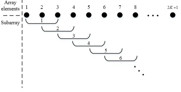
The rotation invariant features of the virtual ULA can be obtained from Eq. (22). Unlike the traditional ULA, the virtual ULA needs at least three subarrays to get the rotation invariant features. MI-ESPRIT algorithm is a type of ESPRIT algorithm using more than one rotation invariant feature of the array. As the virtual ULA obtained from the mode-space transformation is different from the standard ULA, its rotation invariant features need at least three subarrays which must meet the recursive nature shown in Eq. (22). This paper proposes an approach of selecting the subarrays of MI-ESPRIT algorithm, shown in Fig. 2.
In Fig. 2, the virtual ULA is divided intoQsubarrays, and each subarray containskarray elements. There are k−1 overlapping elements between the adjacent subarrays. According to the theory in Section 3.2, the spatial time-frequency matrix of the array output is equal to the autocorrelation matrix in the traditional subspace algorithms, so we can carry through eigen decomposition for the spatial time-frequency matrix, namely:
Figure 2. The schematic diagram of selecting the subarrays withk= 3.
In Eq. (24), WSS is the spatial time-frequency matrix of the signals. WNN is the spatial time-frequency matrix of the noises. U is the signal subspace, which is expanded by the eigen vectors corresponding toM0 large eigenvalues obtained from the Eigen decomposition ofW.
The signal subspace of each subarray can be cut out fromU, namely:
Ul=U(l:l+k−1,:) (26)
In Eq. (25),l is the sequence number of the subarray.
As can be seen from Eq. (22), the three adjacent subarrays in Fig. 2 meet the recursive nature, and the calculation is simple. Assuming three adjacent k×M0 subarrays, the following expressions can be obtained.
[ Ul−1 Ul+1 ]F = LlUl (27)
F = [ c c∗ ]T (28)
Ll = 2diag{ −k+l−1 . . . −K+l+k−2 } (29) In Eq. (26),Ul−1,Ul and Ul+1 are the signal subspaces of these three subarrays, respectively. In order to get the multiple rotation invariant features of the virtual ULA, we can combinehsignal subspaces, namely:
˜
U= [ U1 U2 . . . Uh ]T , h≤Q (30) According to the dividing method shown in Fig. 2, we can see that h must satisfy the following expression.
3≤h≤2K+ 2−k (31)
In this way, we can make use of ˜U to obtain the multiple invariant equation shown in Eq. (26), namely:
UacF = Ub (32)
Uac = [ Ua Uc ] =
U1 U2 . . . Uh−2
U3 U4 . . . Uh T
(33)
Ub = [ L2U2 L3U3 . . . Lh−1Uh−1 ] (34) We can use the MLS criterion to get the closed-form solution of Eq. (31), namely:
FMLS=U+acUb (35)
In Eq. (34),+ represents the generalized inverse matrix.
respectively are λ1i(i= 1,2, . . . , M0) and λ2i(i= 1,2, . . . , M0). So the 2-D DOA estimation of theith LFM signal is as follows.
˜
θi = arg(λ1i/λ2i)/2 (36)
˜
ϕi = arcsin
real(λ1i) + real(λ2i) 4πrficos ˜θi c
(37)
In Eqs. (35) and (36), arg( ) represents a phase angle function of a plural, and real( ) means to take the real part of a plural.
As can be seen from Eq. (31), the multiple rotational invariant equation of the UCA-TF-MI-ESPRIT algorithm is related tokand hafter the virtual ULA is determined. If we select the subarrays using the method shown in Fig. 2, the number of subarrays must satisfy Eq. (30). When h = 3, the UCA-TF-MI-ESPRIT algorithm is the UCA-TF-ESPRIT algorithm. Whenh= 2K+ 2−k, the UCA-TF-MI-ESPRIT algorithm uses all the subarrays, which means using all the rotational invariances of the array. When 3 < h < 2K + 2−k, the UCA-TF-MI-ESPRIT algorithm uses partial rotational invariances of the array.
Whenh = 2K+ 2−k, we can get a total of 2K−1 ways to divide the array with differentkand
h. According to Eq. (31), we can see that the first K methods construct the same rotational invariant equations as the secondK methods, so we can get a total ofK different ways to divide the array with different kand h.
When 3 < h < 2K + 2−k, the UCA-TF-MI-ESPRIT algorithm just utilizes partial rotational invariances of the array. In this case, when one of k and h is determined, the other can be arbitrarily selected within the range formed by 3< h <2K+ 2−k.
For the readers’ convenience, we propose a complete procedure of the UCA-TF-MI-ESPRIT algorithm in Table 1.
Table 1. The complete procedure of the UCA-TF-MI-ESPRIT algorithm.
1) The UCA is equalized to be a virtual ULA based on (14).
2) The SPWVD of the virtual ULA output is calculated based on (16). 3) The spatial time-frequency matrix is obtained based on (19).
4) Carry through eigen decomposition for the spatial time-frequency matrix and get the signal subspace based on (24).
5) Select subarrays based on Fig. 2 and get the signal subspace of each subarray based on (25). 6) Get the multiple invariant equation based on (31).
7) Get the closed-form solution of (31), which isFMLS.
8) Carry through eigen decomposition forFMLS and get the 2-D DOA estimation based on (35) and (36). 9) IfM0 < M, repeat 3)–8) until all the signals’ DOA are estimated. IfM0 =M, all the signals’
DOA are already estimated and the algorithm procedure is over. Among them, M is the number of incident waves andM0 is the number of the signals included in the time-frequency matrix.
4. NUMERICAL SIMULATION
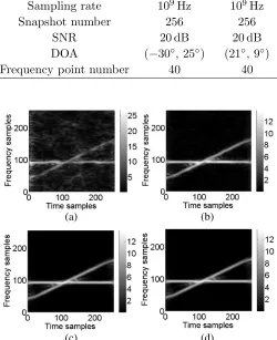
Table 2. The parameters table of far-field signals.
Symbol Value Value
Signal number 1 2
Initial frequency 1.8×10⁹Hz 7×10⁸Hz Modulated frequency 0 1016Hz/s
Sampling rate 109Hz 109Hz
Snapshot number 256 256
SNR 20 dB 20 dB
DOA (−30◦,25◦) (21◦, 9◦)
Frequency point number 40 40
(a) (b)
(c) (d)
Figure 3. The SPWVD results of the eighth element. (a) is the SPWVD results when SNR is−10 dB. (b) is the SPWVD results when SNR is 0 dB. (c) is the SPWVD results when SNR is 10 dB. (d) is the SPWVD results when SNR is 20 dB.
As can be seen from Fig. 3, the single frequency signal and LFM signal both possess ideal energy collection features in the time-frequency plane. Even in the case of low SNR (−10 dB), SPWVD can also gather the signal energy in the time-frequency plane obviously. The cross-term interferences are basically removed by using SPWVD. There are only sporadic cross-term interferences existing in certain time-frequency points near the multi-source time-time-frequency points. So the interferences have little influence on subsequent DOA estimation.
We select 40 time-frequency points located in the middle of the time window to obtain the spatial time-frequency matrix base on Eq. (19). Then we carry through eigen decomposition for the matrix and get the signal subspace. We use UCA-WVD-MI-ESPRIT algorithm withk= 4 andh= 12 to carry through DOA estimation, and the results are (−29.93◦,25.02◦) and (21.08◦,8.89◦), respectively. The estimates are matched with the DOA set in Table 2.
error and the elevation angle estimation error, namely:
RMSE =
1
num num
j=1
( ˜θj−θ)2+ ( ˜ϕ
j−ϕ)2 (38)
In Eq. (36), num stands for the number of Monte Carlo simulations. θ˜j is the azimuth angle estimation of the jth simulation and ˜ϕj the elevation angle estimation of thejth simulation.
In addition to an incremental SNR of the signals, the other parameters remain unchanged. We carry through a total of 1000 times of Monte Carlo simulation, and the results are shown in Fig. 4.
Figure 4 shows the estimation RMSE of the two signals along with SNR. As can be seen from the figure, the RMSE of DOA estimations decrease rapidly with the increase of the signals’ SNR and achieve the convergence condition (The RMSE is infinitely close to zero) ultimately. In the low SNR (less than 0 dB) situation, the RMSEs of the two signals are still less than 1.8◦, so the UCA-TF-MI-ESPRIT algorithm also owns a good estimation precision in the case of low SNR. For a UCA, the precision of DOA estimation for the waves of different directions has isotropy in theory; however, we use the approximation in Eq. (6) when carrying through the mode-space transformation. The precisions of extracting different signals’ time-frequency points are not the same due to random errors, so the DOA estimation precisions for the waves of different directions are not the same. The simulation results are in line with expectations.
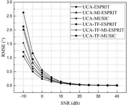
In order to further examine the performance of the algorithm, we carry through the comparison simulation between ESPRIT algorithm in [11], MI-ESPRIT algorithm in [13], UCA-MUSIC algorithm in [6], UCA-TF-ESPRIT algorithm in [20], UCA-TF-UCA-MUSIC algorithm [18] and the algorithm proposed by this paper. Among them, UCA-MI-ESPRIT algorithm and UCA-TF-MI-ESPRIT algorithm both use 12 subarrays, and each subarray contains 4 elements. We select signal 1 in Table 2 as the incoming signal, and the parameters of UCA are unchanged. We carry out a total of 1000 times of Monte Carlo simulation, and the results are shown in Fig. 5.
Figure 5 shows the estimation RMSE along with SNR of signal 1 when using six different algorithms. As can be seen from the figure, the RMSE decreases rapidly with the increase of the signal’s
Figure 4. RMSE of DOA estimation along with SNR. The UCA-TF-MI-ESPRIT algorithm uses
k = 4 and h = 12 to estimate the DOA of two signals in Table 2.
SNR and achieves the convergence condition ultimately. In general, the UCA-TF-MUSIC algorithm owns the highest estimation precision, followed by the UCA-MUSIC algorithm, UCA-TF-MI-ESPRIT algorithm, UCA-MI-ESPRIT algorithm, UCA-TF-ESPRIT algorithm and UCA-ESPRIT algorithm. The estimation precision of the UCA-TF-MI-ESPRIT algorithm is improved a lot compared to the UCA-TF-ESPRIT algorithm and UCA-MI-ESPRIT algorithm. Especially in the case of low SNR, the precision improvement is very obvious (When SNR is−10 dB, the RMSE of DOA estimation is reduced more than 0.6◦). Although the estimation accuracy of MUSIC-like algorithms is better than the UCA-TF-MI-ESPRIT algorithm, the superiority is not big. When SNR is−10 dB, the estimation RMSE of the UCA-MUSIC algorithm is reduced only about 0.25◦ compared to the UCA-TF-MI-ESPRIT algorithm, and the estimation RMSE of the UCA-TF-MUSIC algorithm is reduced only about 0.4◦ compared to the UCA-TF-MI-ESPRIT algorithm. When the SNR is −5 dB, the reduced value of RMSE becomes 0.1◦ and 0.2◦, respectively. With the increase of signal’s SNR, the estimation RMSEs of these three algorithms tend to be the same (When SNR is higher than 0 dB, the three RMSE curves are basically coincident), which means that the DOA estimation precisions of three algorithms tend to be the same. Although the estimation precision of the UCA-TF-MI-ESPRIT algorithm is slightly lower than that of MUSIC-like algorithms, its computational complexity is much lower. MUSIC-like algorithms need to search the spectrum peak. In order to obtain a high estimation precision, we need select a small search step angle. In the case of 2-D DOA estimation, it will cause a pretty high computational complexity. In this simulation, the searching step of the azimuth angle and elevation angle are both 0.01◦. The searching range in the azimuth direction is from−180◦ to 180◦, and the searching range in the elevation direction is from −90◦ to 90◦. So the number of data points will be over 6×10⁹ when searching the spectrum peak, which will bring about a very large burden for the algorithm’s operation speed and data storage. The UCA-TF-MI-ESPRIT algorithm only needs to construct a multiple rotational invariant equation and get the closed solution. So its computational complexity is basically comparative to the standard ESPRIT algorithm. In conclusion, the UCA-TF-MI-ESPRIT algorithm owns an obvious advantage in terms of computational complexity compared to MUSIC-like algorithms, and it also owns an obvious advantage in terms of estimation precision compared to the traditional ESPRIT-like algorithms.
As can be seen form the deduction of Section 3.2, when the element number of the virtual ULA is determined, k andh will determine the multiple invariant equation shown in Eq. (31), which means that the DOA estimation results using the UCA-TF-MI-ESPRIT algorithm are related to kand h. In this paper, we simulate the relationship between the estimation precision of the UCA-TF-MI-ESPRIT algorithm and the values of k and h. We select signal 1 in Table 2 as the incoming signal, and the parameters of UCA are unchanged. We perform a total of 1000 times of Monte Carlo simulation, and the results are shown in Fig. 6.
Figure 6(a) shows the DOA estimation RMSE along with signal’s SNR withh= 8 andkincreased
(a) (b)
from 1 to 8. Fig. 6(b) shows the DOA estimation RMSE along with signal’s SNR with k = 4 and
h increased from 5 to 12. In the figure, k = 8, h = 8 and k = 4, h = 12 satisfy h = 2K+ 2−k, which means that the algorithm uses all the rotational invariances of the array. The other cases satisfy 3 < h < 2K + 2−k, which means that the proposed algorithm uses partial rotational invariances of the array. As can be seen from the results shown in Fig. 7, the estimation RMSE decreases with the increase of signal’s SNR or k or h. When k or h is small or SNR is low, the reduction of RMSE is more obvious. With the increase ofkorh or SNR, the DOA estimation precision differences tend to be consistent in different cases. In Fig. 6(a), the RMSE difference between k= 1, h= 8 andk= 2, h= 8 is about 0.9161◦; however, the RMSE difference between k= 7, h = 8 andk= 8, h = 8 is just about 0.0373◦. When SNR is 10 dB, the RMSE difference betweenk = 1, h = 8 and k = 2, h = 8 is about 0.0479◦; however, the RMSE difference betweenk= 7,h= 8 andk= 8,h= 8 is just about 0.0041◦. In Fig. 6(b), the RMSE difference between k= 4, h= 5 and k= 4, h = 6 is about 1.1262◦; however, the RMSE difference betweenk= 4, h= 11 andk= 4,h= 12 is just about 0.0973◦. When SNR is 10 dB, the RMSE difference between k = 4, h = 5 and k = 4, h = 6 is about 0.0672◦; however, the RMSE difference between k = 4, h = 11 and k = 4, h = 12 is just about 0.0024◦. So, when the proposed algorithm uses partial rotational invariances of the array, ifkorh is a constant value, with the increase of h ork, the DOA estimation precision becomes closer to the estimation precision when using all the rotational invariances of the array. In this simulation, after k = 6 with h = 8 or h = 10 with k = 4, the estimation precisions of using partial rotational invariances and all the rotational invariances are basically the same.
We can see from Eq. (31) that the largerk and h are, the higher the computational complexity of the algorithm is, which means that the algorithm has the highest computational complexity when using all the rotational invariances of the array. Therefore, the UCA-TF-MI-ESPRIT algorithm can perform DOA estimation using partial rotational invariances of the array, which can reduce the computational complexity of the proposed algorithm while maintaining the estimation precision basically.
5. CONCLUSION
This paper proposes a new DOA estimation algorithm of multiple LFM signals for UCA based on mode-space algorithm and TF-MI-ESPRIT algorithm, which is called UCA-TF-MI-ESPRIT algorithm. A simple and effective subarray dividing approach is also proposed in the paper when constructing the multiple invariance of the array. The algorithm uses SPWVD instead of WVD as the time-frequency analysis tool to retrain the cross-term interferences. It can be applied to the UCA to realize 2-D DOA estimation of multiple LFM signals. On the basis of keeping the low computational complexity of ESPRIT class algorithms, the UCA-TF-MI-ESPRIT algorithm increases the DOA estimation precision. Especially in the case of low SNR, the estimation precision has a big enhancement compared to the traditional ESPRIT algorithm. The numerical simulations verify the effectiveness of the algorithm and conclude the influences of the subarray numbers and the subarray element numbers on the DOA estimation precision, which provides a good basis for the application of the algorithm.
REFERENCES
1. Du, W., D. L. Su, S. G. Xie, and H. T. Hui, “A fast calculation method for the receiving mutual impedances of uniform circular arrays,”IEEE Antennas and Wireless Propagation Letters, Vol. 11, No. 2, 893–896, Aug. 2012.
2. Liao, B., K. M. Tsui, and S. C. Chan, “Frequency invariant uniform concentric circular arrays with directional elements,” IEEE Transactions on Aerospace and Electronics Systems, Vol. 49, No. 2, 871–884, Apr. 2013.
3. Jackson, B. R., S. Rajan, B. J. Liao, and S. C. Wang, “Direction of arrival estimation using directive antennas in uniform circular arrays,” IEEE Transactions on Antennas and Propagation, Vol. 63, No. 2, 736–747, Feb. 2015.
5. Wang, M., X. C. Ma, S. F. Yan, and C. P. Hao, “An autocalibration algorithm for uniform circular array with unknown mutual coupling,” IEEE Antennas and Wireless Propagation Letters, Vol. 15, 12–15, Apr. 2015.
6. Schmidt, R. O., “Multiple emitter location and signal parameter estimation,” IEEE Transactions on Antennas and Propagation, Vol. 34, No. 3, 276–280, Mar. 1986.
7. Roy, R. and T. Kailath, “ESPRIT — A subspace rotation approach to estimation of parameters of cisoids in noise,” IEEE Transactions on Acoustics, Speech, and Signal Processing, Vol. 34, No. 5, 1340–1342, Oct. 1986.
8. Roy, R. and T. Kailath, “ESPRIT-estimation of signal parameters via rotational invariance techniques,” IEEE Transactions on Acoustics, Speech, and Signal Processing, Vol. 37, No. 7, 984– 995, Jul. 1989.
9. Wang, Y. L., H. Chen, Y. N. Peng, and Q. Wan, Spatial Spectrum Estimation, 340–346, Tsinghua University Press, Beijing, China, 2004.
10. Griffiths, H. D. and R. Eiges, “Sectoral phase modes from circular antenna arrays,” Electronics Letters, Vol. 28, No. 17, 1581–1582, Aug. 1992.
11. Zoltowski, M. D. and C. P. Mathews, “Closed-form 2D angle estimation with uniform circular arrays via phase mode excitation and ESPRIT,”The 27th Asilomar Conference on Signals, Systems and Computers, 169–173, Los Alamitos, USA, 1993.
12. Swindlehurst, A. L., B. Ottersten, R. Roy, and T. Kailath, “Multiple invariance ESPRIT,” IEEE Transactions on Signal Processing, Vol. 40, No. 4, 867–881, Apr. 1992.
13. Xu, Y. G. and Z. W. Liu, “Closed-form multiple invariance ESPRIT,”Multidim Syst. Sign Process, Vol. 18, 47–54, Feb. 2007.
14. Zhang, X. F., X. Gao, and D. Z. Xu, “Multi-invariance ESPRIT based blind DOA estimation for MC-CDMA with an antenna array,” IEEE Transactions on Vehicular Technology, Vol. 58, No. 8, 4686–4690, Oct. 2009.
15. Tang, X. H. and Q. L. Li,Time Frequency Analysis and Wavelet Transform, 82–118, Science Press, Beijing, China, 2016.
16. Amin, M. G., “Spatial time frequency distributions for direction finding and blind source separation,” The International Society for Optical Engineering (Proc. SPIE), Vol. 3723, 62–70, Orlando, USA, 1999.
17. Belouchrani, A. and M. G. Amin, “Blind source separation based on time-frequency signal representations,” IEEE Transactions on Signal Processing, Vol. 46, No. 11, 2888–2897, Nov. 1998. 18. Belouchrani, A. and M. G. Amin, “Time frequency MUSIC,” IEEE Signal Processing Letters,
Vol. 6, No. 5, 109–110, May 1999.
19. Gershman, A. B. and M. G. Amin, “Wideband direction-of-arrival estimation of multiple chirp signals using spatial time-frequency distributions,” IEEE Signal Processing Letters, Vol. 7, No. 6, 152–155, Jun. 2000.
20. Zhang, Y. M., W. F. Mu, and M. G. Amin, “Subspace analysis of spatial time-frequency distribution matrices,”IEEE Transactions on Signal Processing, Vol. 49, No. 4, 747–759, Apr. 2001.
21. Nguyen, L. T., B. Adel, A. M. Karim, and B. Boualem, “Separating more sources than sensors using time-frequency distributions,”EURASIP Journal on Applied Signal Processing, Vol. 17, 2828–2847, Jul. 2005.
22. Abdeldjalil, A. E. B., L. T. Nguyen, A. M. Karim, B. Adel, and G. Yves, “Underdetermined blind separation of nondisjoint sources in the time-frequency domain,” IEEE Transactions on Signal Processing, Vol. 55, No. 3, 897–907, Mar. 2007.
23. Zhang, Y. M. and M. G. Amin, “Blind separation of nonstationary sources based on spatial time-frequency distributions,” EURASIP Journal on Applied Signal Processing, Vol. 2006, 1–13, Aug. 2006.
25. Mohamed, K., B. Adel, and A. M. Karim, “Performance analysis for time-frequency MUSIC algorithm in presence of both additive noise and array calibration errors,” EURASIP Journal on Advances in Signal Processing, Vol. 94, 1–11, Apr. 2012.
26. Lin, J. C., X. C. Ma, S. F. Yan, and C. P. Hao, “Time-frequency multi-invariance ESPRIT algorithm for DOA estimation,” IEEE Antennas and Wireless Propagation Letters, Vol. 15, 770– 773, Aug. 2015.
27. Lin, M. and L. Yang, “Blind calibration and DOA estimation with uniform circular arrays in the presence of mutual coupling,” IEEE Antennas and Wireless Propagation Letters, Vol. 5, No. 1, 315–318, Jul. 2006.
28. Wu, Y. T. and H. C. So, “Simple and accurate two-dimensional angle estimation for a single source with uniform circular array,” IEEE Antennas and Wireless Propagation Letters, Vol. 7, No. 1, 78–80, Apr. 2008.